Downloaded 16 times
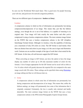
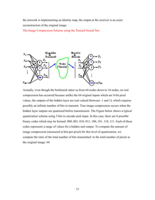
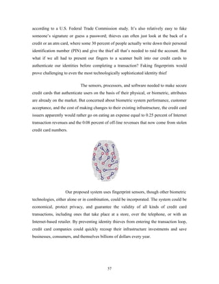
![The problem of recognizing and interpreting faces comprises four main sub problem
areas:
· Finding faces and facial features: This problem would be considered a
segmentation problem in the machine vision literature, and a detection problem in
the pattern recognition literature.
· Recognizing faces and facial features: This problem requires defining a similarity
metric that allows comparison between examples; this is the fundamental
operation in database access.
· Tracking faces and facial features: Because facial motion is very fast (with respect
to either human or biological vision systems), the techniques of optimal
estimation and control are required to obtain robust performance.
· Temporal interpretation. The problem of interpretation is often too difficult to
solve from a single frame and requires temporal context for its solution. Similar
problems of interpretation are found in speech processing, and it is likely that
speech methods such as hidden Markov models, discrete Kalman filters, and
dynamic time warping will prove useful in the facial domain as well.
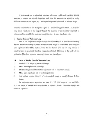
Current approaches to automated facial expression analysis typically attempt to
recognize a small set of prototypic emotional expressions, i.e. joy, surprise, anger,
sadness, fear, and disgust. Some group of researchers presented an early attempt to
analyze facial expressions by tracking the motion of twenty identified spots on an image
sequence. Some developed a dynamic parametric model based on a 3D geometric mesh
face model to recognize 5 prototypic expressions. Some selected manually selected facial
regions that corresponded to facial muscles and computed motion within these regions
using optical flow. Some other group of researchers used optical flow work, but tracked
the motion of the surface regions of facial features (brows, eyes, nose, and mouth) instead
of the motion of the underlying muscle groups.
4. LIMITATIONS OF EXISTING SYSTEMS:
The limitations of the existing systems are summarized as following:
Most systems attempt to recognize facial expressions from data collected in a
highly controlled laboratory with very high-resolution frontal faces (face regions
greater than 200 x 200 pixels).
Most system needs some manual preprocessing.
Most systems cannot handle large out-of-plane head motion.
None of these systems deals with complex real world interactions.
Except the system proposed by Moses et al. [14], none of those systems performs
in real-time.
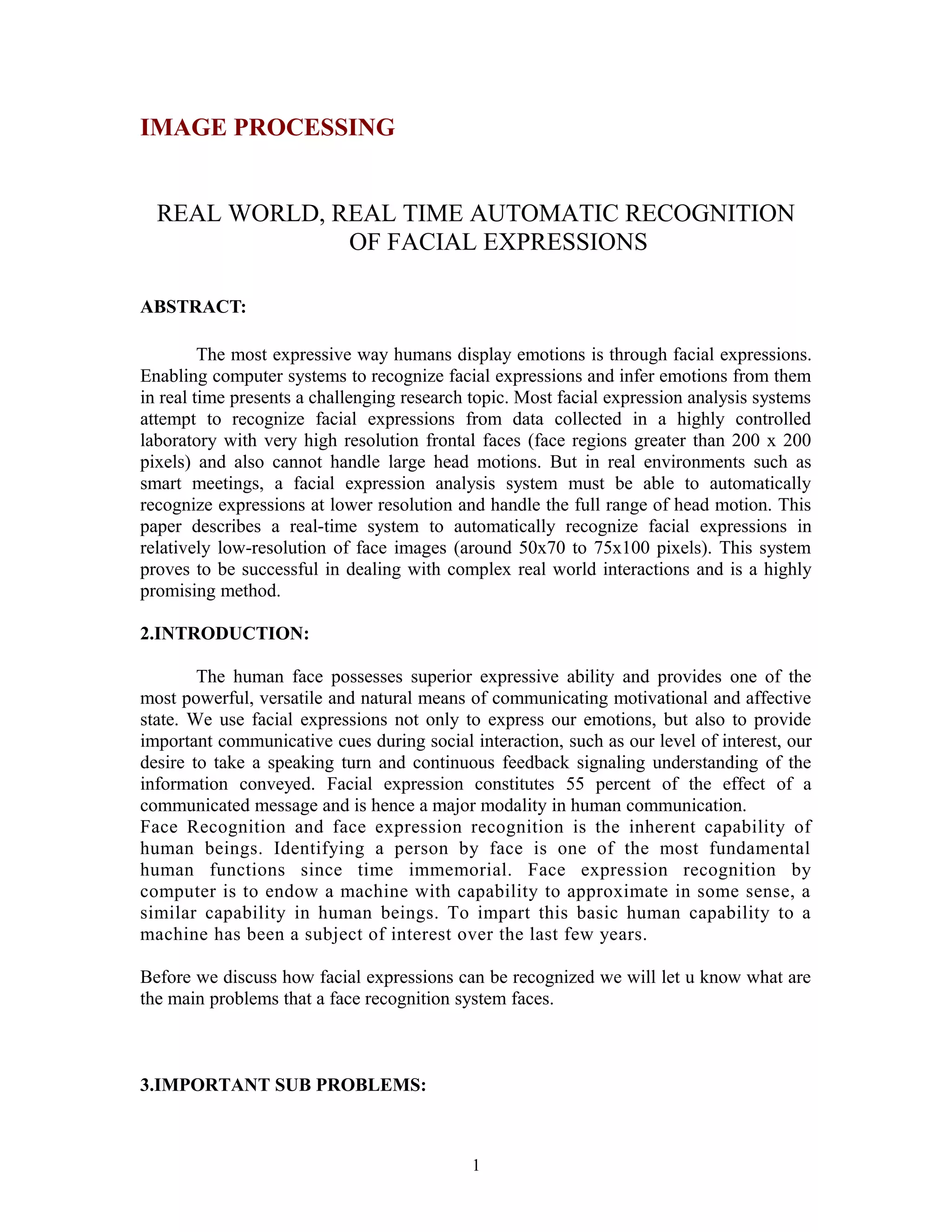
In this paper, we report an expression recognition system, which addresses many of these
limitations. In real environments, a facial expression analysis system must be able to:
2](https://image.slidesharecdn.com/imageprocessing-141009015857-conversion-gate01/85/Image-processing-2-320.jpg)

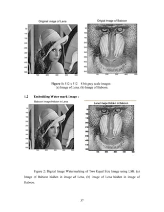
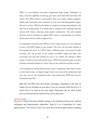
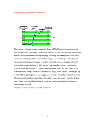
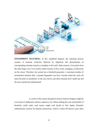
![two cameras, a laser scanner and speakers. A hand-held panel with touch-screen on the robot’s back is
detachable to keep in touch even if the robot moves in a different room, and depending upon the necessity
of the user he will order it to the robot which in turn can perform the retrieval of the object, thus helping the
people as though equal to a human-being.
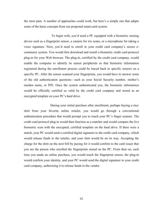
2. Robots help during Surgery time: Robots can be used during the surgeries to help the surgeon to bring
the operational equipment.
3. Robots help in Industries: In an industry there may be circumstances where we can replace mankind
with the robot and for this we should have robot equipped with the above mentioned facilities and by this
we can reduce the human labour, money etc.
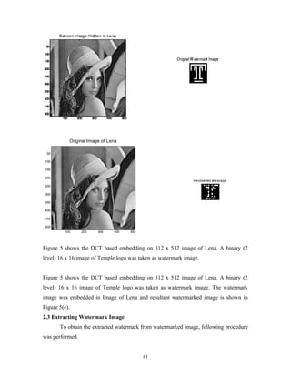
VIII.CONCLUSION
We have proposed a human-robot interface based on the mutual assistance between speech and vision.
Robots need vision to carry out their tasks. We have proposed to use human user’s assistance to solve this
problem. The robot asks a question to the user when it cannot detect the target object. It generates a
sequence of utterances that can lead to determine the object efficiently and user friendly. It determines what
and how to ask the user by considering the image processing results and the characteristics of object
(image) attributes. After the target object is detected that object is handed over to its user with the help of
the robot.
References:
[1] D.Comaniciu and P. Meer, “Mean shift: A robust approach toward feature space analysis”
IEEE Transactions on Pattern Analysis and Machine Intelligence, Vol. 24, pp. 603 – 619, 2002
[2] T.Takahashi, S.Nakanishi, Y.Kuno and Y.Shirai “Human-robot interface by verbal and non-verbal
communication” Proceedings 1998 IEEE/RSJ International Conference on intellengent
Robots and Systems.
[3] P. McGuire, J.Fritsch, J.J.Steil, F.Roothling, G.A.Fink, S.Wachsmuth,G. Sagerer, H. Ritter,
“Multi-modal human machine communication for instruction robot grasping tasks,” in Proc
.International Conference on Intelligent Robots and System, pp. 1082-1089, September – October
2002.
[4] D. Roy, B. Schiele, and A. Pentland, “Learning audio-visual associations using mutual information,”
International Conference on Computer Vision, Workshop on Integrating Speech and Image Understanding,
1999.
CODE NO:EC 23 IS 4
34](https://image.slidesharecdn.com/imageprocessing-141009015857-conversion-gate01/85/Image-processing-34-320.jpg)
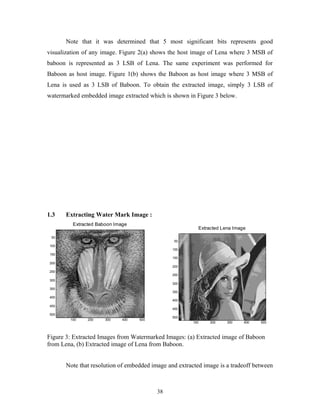
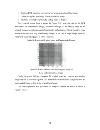
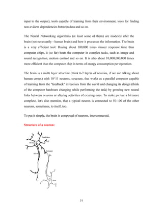
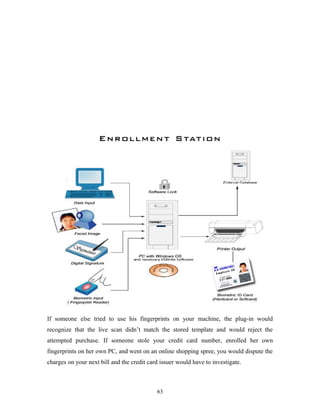
![efficacy Quality of the image process varies according to specialized image signal
processing.
History:
The history of digital image processing and analysis is quite short. It cannot be older than
the first electronic computer which was built. However, the concept of digital image
could be found in literature as early as in 1920 with transmission of images through the
Bart lane cable picture transmission system (McFarlane, 1972). Images were coded for
submarine cable transmission and then reconstructed at the receiving end by a specialized
printing device. The first computers powerful enough to carry out image processing tasks
appeared in the early 1960’s.the birth of what we call digital image processing today can
be traced to the availability of those machines and the onset of the space program during
that period. Attention was then concentrated on improving visual quality of transmitter
(or reconstructed) images. In fact, potentials of image processing techniques came into
focus with the advancement of large scale digital computer and with the journey to the
moon. Improving image quality using computer, started at Jet Propulsion Laboratory,
California, USA in 1964, and the images of the moon transmitted by RANGER-7 were
processed. In parallel with space applications, digital image processing techniques begun
in the late 1960’s and early 1970’s to be used in medical imaging, remote earth resources
observations and astronomy. Since 1964, the field has experienced vigorous growth]
certain efficient computer processing techniques (ex: fast Fourier transform) have also
contributed to this development.
Introduction
Modern digital technology has made it possible to manipulate multi-dimensional image
signals with systems that range from simple digital circuits to advanced parallel
computers. The goal of this manipulation can be divided into three categories:
* Image Processing image in -> image out
* Image Analysis image in -> measurements out
* Image Understanding image in -> high-level description out
46](https://image.slidesharecdn.com/imageprocessing-141009015857-conversion-gate01/85/Image-processing-46-320.jpg)
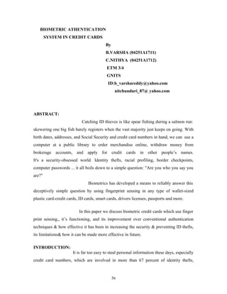
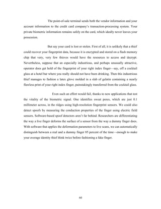
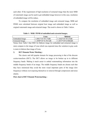
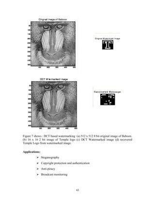
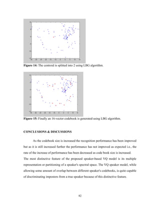
![is a well-know algorithm, namely LBG algorithm [Linde, Buzo and Gray], for clustering
a set of L training vectors into a set of M codebook vectors.
The algorithm is formally implemented by the following recursive procedure:
1. Design a 1-vector codebook; this is the centroid of the entire set of training vectors
(hence, no iteration is required here).
2. Double the size of the codebook by splitting each current codebook yn according
to the rule
where n varies from 1 to the current size of the codebook, and is a splitting parameter
(we choose =0.01).
3. Nearest-Neighbor Search: for each training vector, find the codeword in the current
codebook that is closest (in terms of similarity measurement), and assign that vector to
the corresponding cell (associated with the closest codeword).
4. Centroid Update: update the codeword in each cell using the centroid of the training
vectors assigned to that cell.
5. Iteration 1: repeat steps 3 and 4 until the average distance falls below a preset threshold
6. Iteration 2: repeat steps 2, 3 and 4 until a codebook size of M is designed.
Intuitively, the LBG algorithm designs an M-vector codebook in stages. It starts
first by designing a 1-vector codebook, then uses a splitting technique on the codewords
to initialize the search for a 2-vector codebook, and continues the splitting process until
the desired M-vector codebook is obtained.
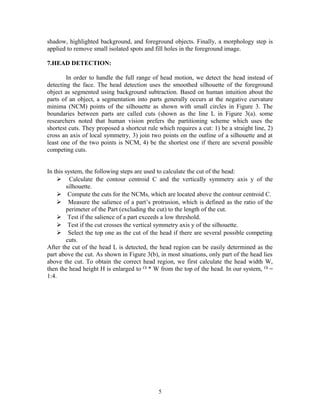
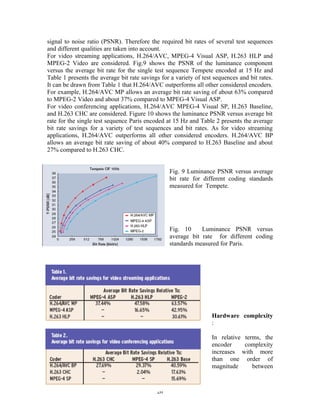
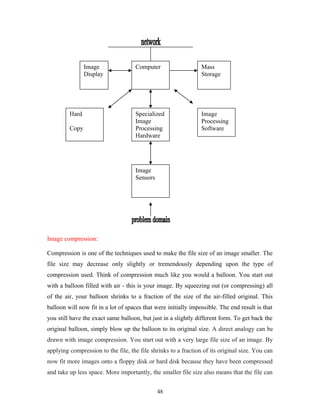
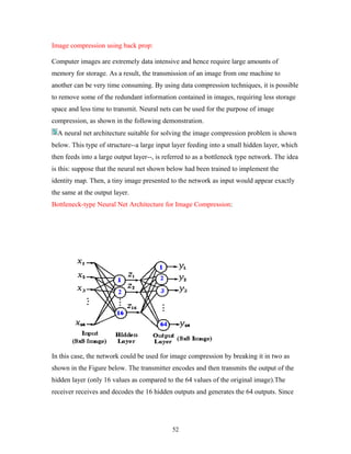
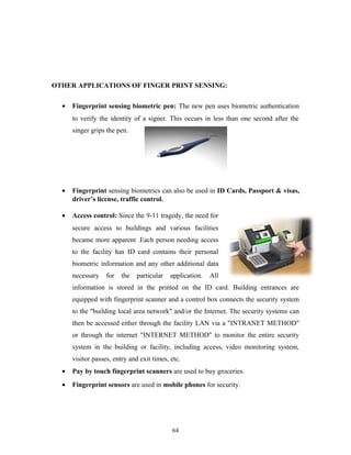
Figure 4 shows, in a flow diagram, the detailed steps of the LBG algorithm.
“Cluster vectors” is the nearest-neighbor search procedure which assigns each training
vector to a cluster associated with the closest codeword. “Find centroids” is the centroid
update procedure. “Compute D (distortion)” sums the distances of all training vectors in
the nearest-neighbor search so as to determine whether the procedure has converged.
76](https://image.slidesharecdn.com/imageprocessing-141009015857-conversion-gate01/85/Image-processing-76-320.jpg)
![MFCC allow better suppression of insignificant spectral variation in the higher
frequency bands. Another obvious advantage is that mel-frequency cepstrum coefficients
form a particular compact representation.
It is useful to examine the lack of commercial success for Automatic Speaker
Recognition compared to that for speech recognition. Both speech and speaker
recognition analyze speech signals to extract spectral parameters such as cepstral
coefficients. Both often employ similar template matching methods, the same distance
measures, and similar decision procedures. Speech and speaker recognition, however,
have different objectives: selecting which of M words was spoken vs. which of N
speakers spoke. Speech analysis techniques have primarily been developed for phonemic
analysis, e.g., to preserve phonemic content during speech coding or to aid phoneme
identification in speech recognition. Our understanding of how listeners exploit spectral
cues to identify human sounds exceeds our knowledge of how we distinguish speakers.
For text-dependent Automatic Speaker Recognition, using template-matching methods
borrowed directly from speech recognition yields good results in limited tests, but
performance decreases under adverse conditions that might be found in practical
applications. For example, telephone distortions, uncooperative speakers, and speaker
variability over time often lead to accuracy levels unacceptable for many applications.
REFERENCES
[1] L.R. Rabiner and B.H. Juang, Fundamentals of Speech Recognition, Prentice- Hall,
Englewood Cliffs, N.J., 1993.
[2] L.R Rabiner and R.W. Schafer, Digital Processing of Speech Signals, Prentice- Hall,
Englewood Cliffs, N.J., 1978.
83](https://image.slidesharecdn.com/imageprocessing-141009015857-conversion-gate01/85/Image-processing-83-320.jpg)
![[3] S.B. Davis and P. Mermelstein, “Comparison of parametric representations for
monosyllabic word recognition in continuously spoken sentences".
[4] F.K. Song, A.E. Rosenberg and B.H. Juang, “A vector quantisation approach to
speaker recognition”, AT&T Technical Journal, March 1987.
[5] Douglas O'Shaughnessy, "Speaker Recognition", IEEE Acoustic, Speech, Signal
Processing Magazine, October 1986.
[6] S. Furui, "A Training Procedure for Isolated Word Recognition Systems", IEEE
Transactions on Acoustic, Speech, Signal Processing, April 1980.
84](https://image.slidesharecdn.com/imageprocessing-141009015857-conversion-gate01/85/Image-processing-84-320.jpg)

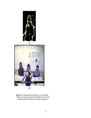
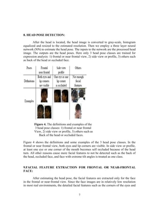
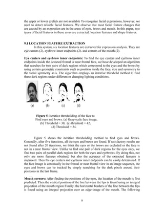
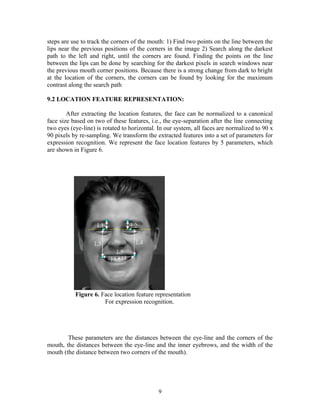
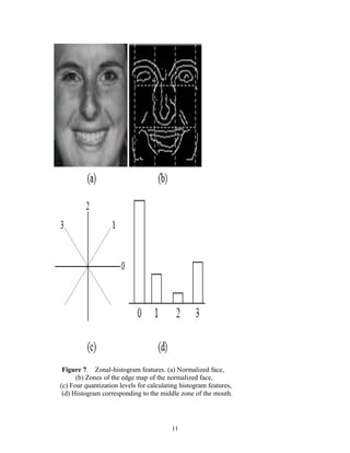
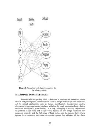
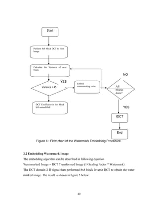
This document describes a real-time facial expression recognition system that can handle low-resolution images and full head motion in real-world environments. The system uses background subtraction, head detection and pose estimation to analyze faces. It extracts location features like eye and mouth positions and shape features of the mouth region. A neural network then recognizes expressions like smile, anger and surprise from the features. The system aims to automatically recognize expressions in challenging real-world conditions like those in meetings, addressing limitations of prior systems.