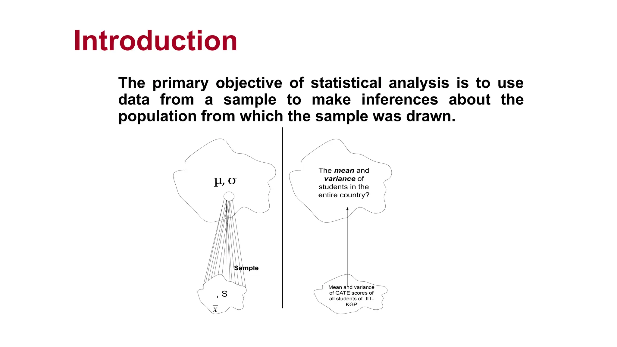
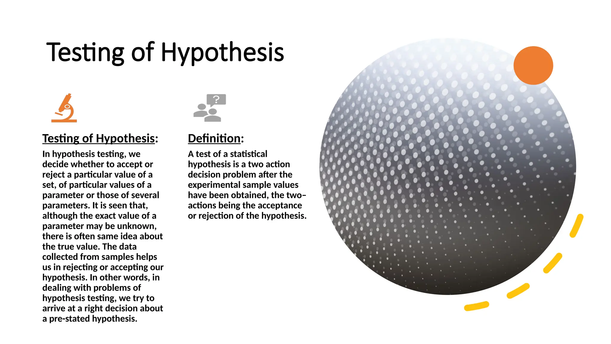
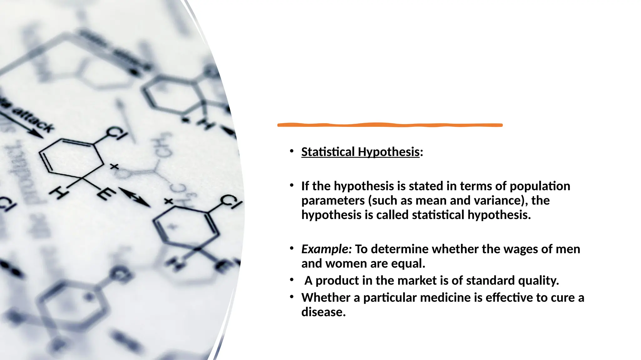
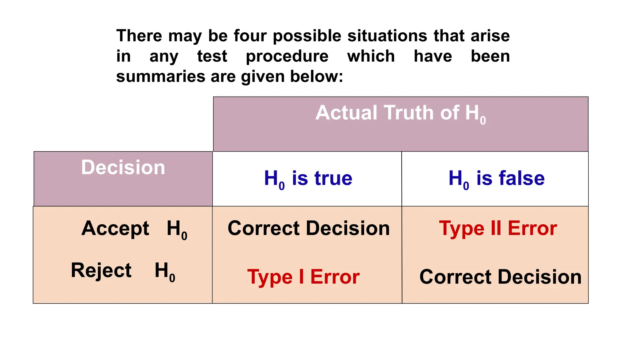
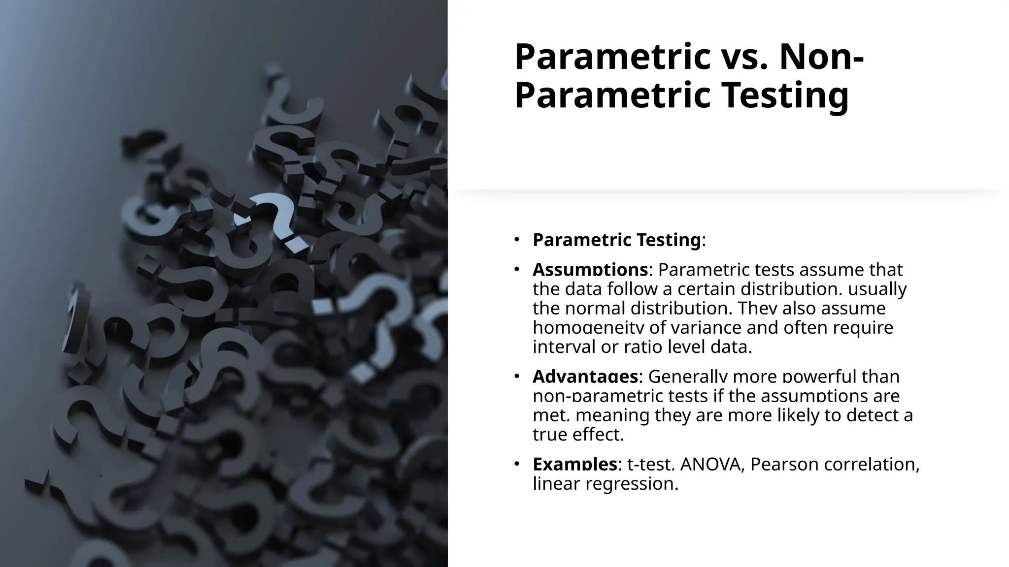
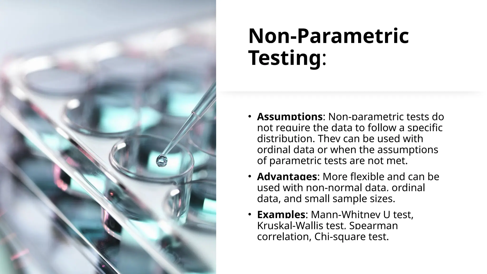
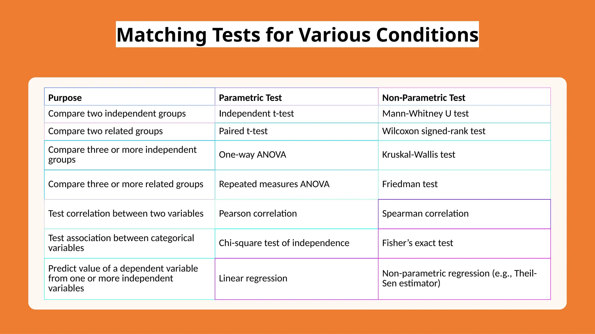
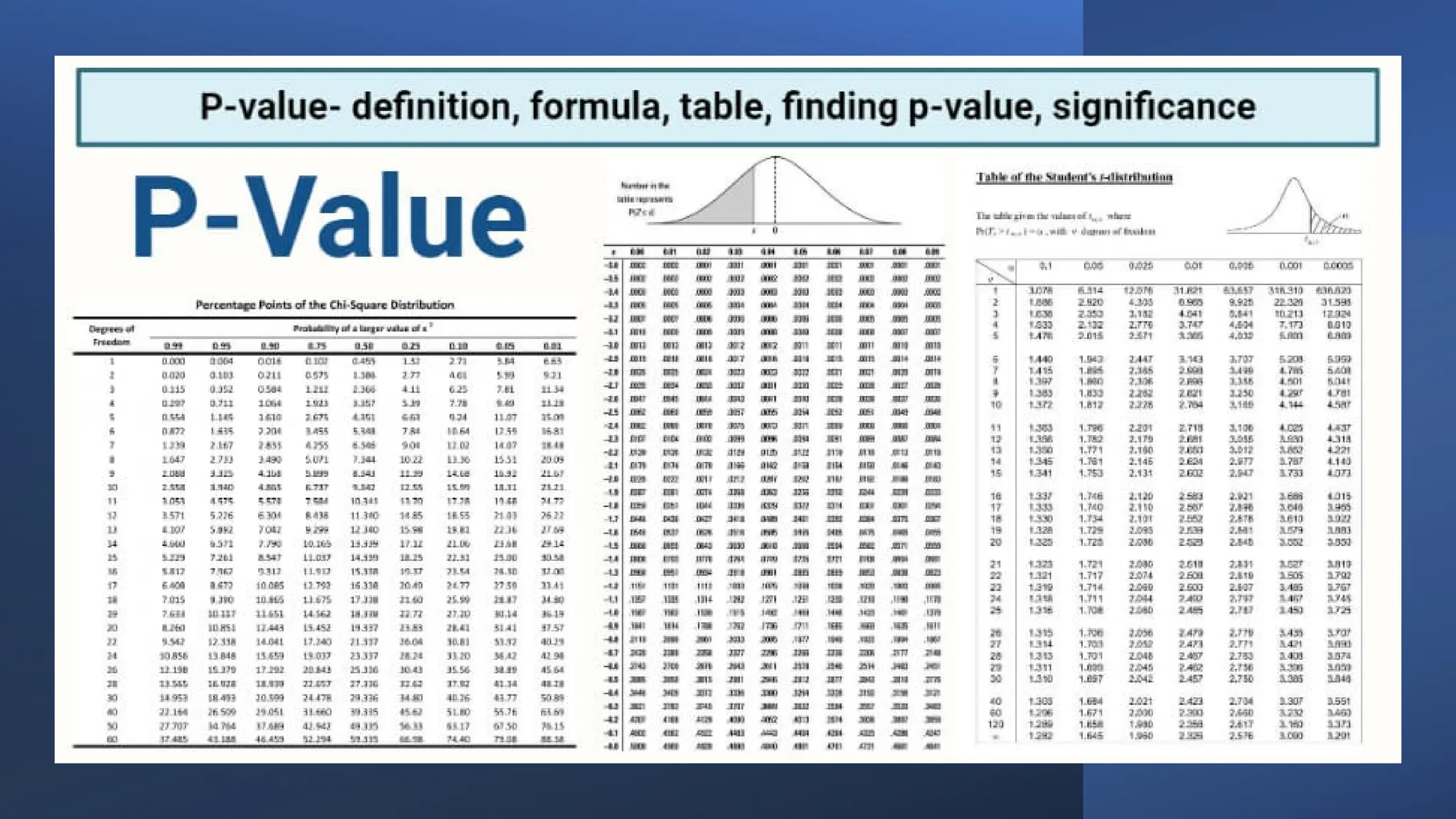
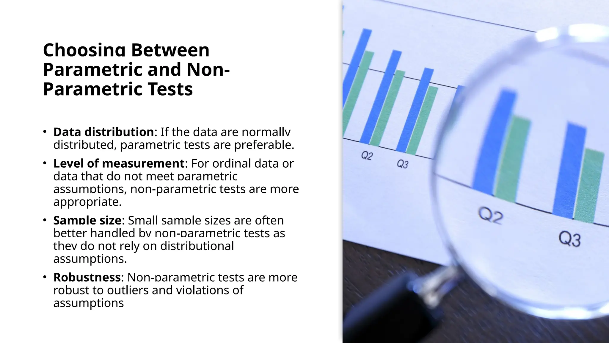
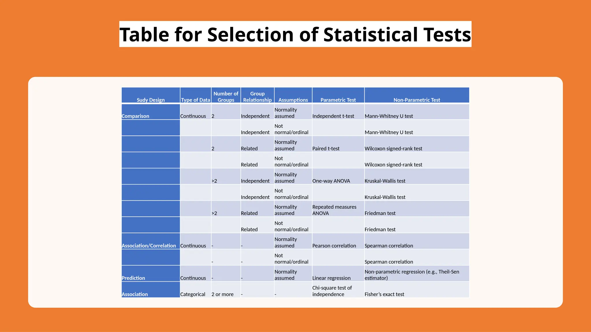
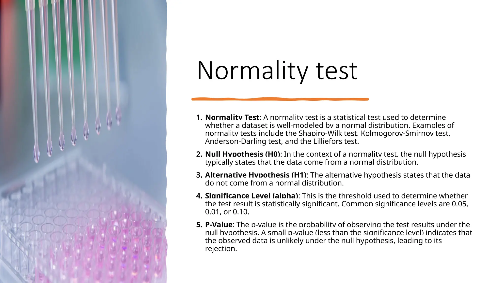
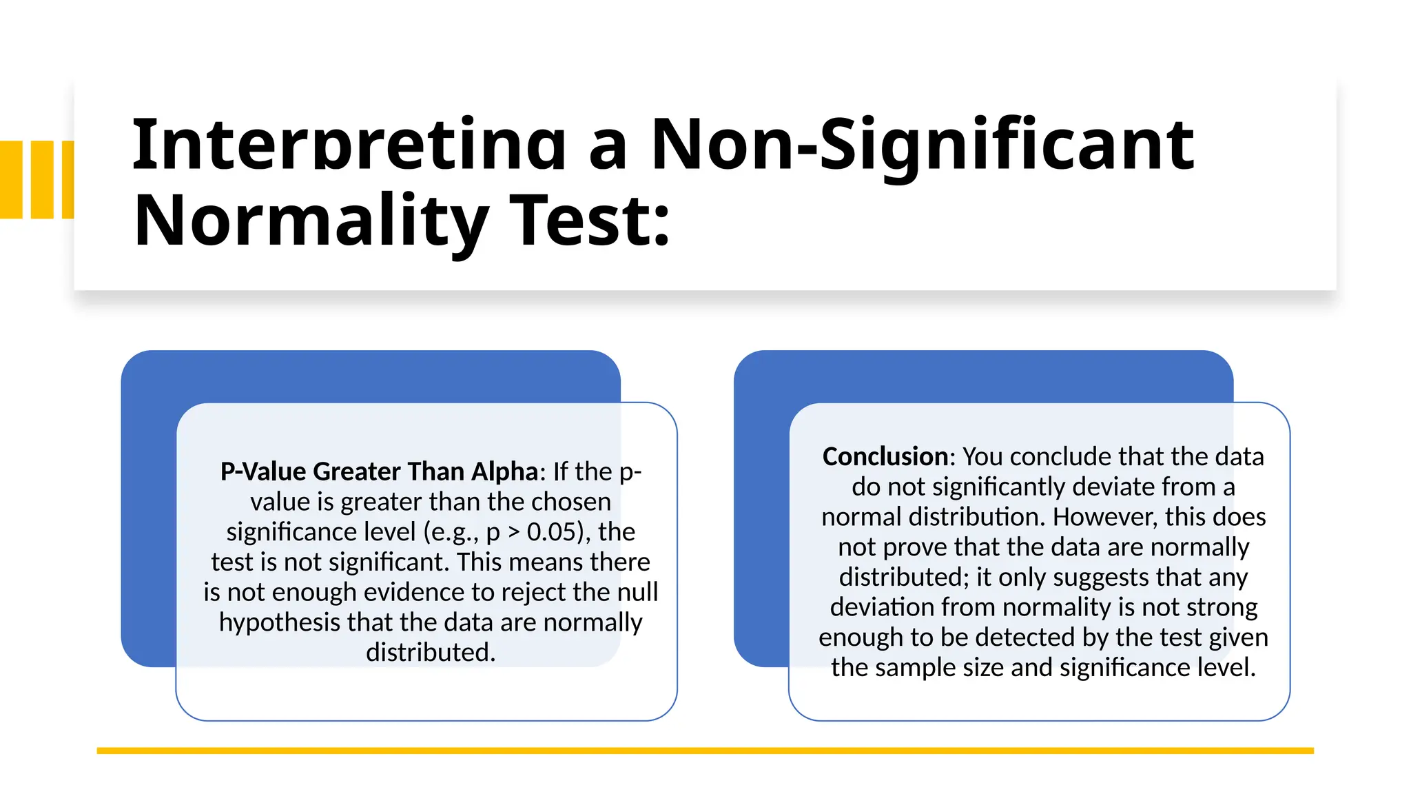
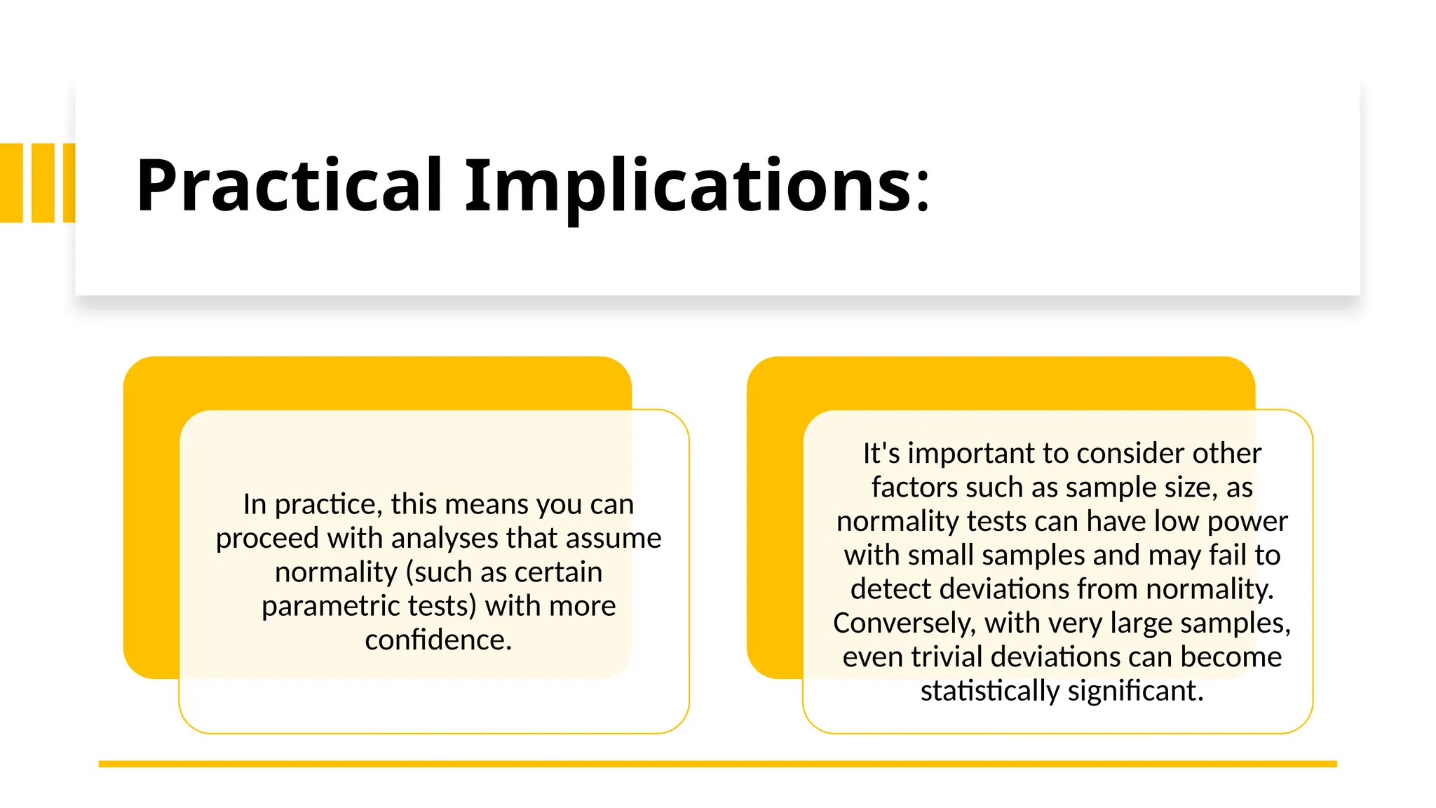
The document discusses hypothesis testing and inference, defining a hypothesis as a testable prediction regarding research outcomes, and outlining characteristics of good hypotheses. It elaborates on types of hypotheses, specifically null and alternative, detailing their roles in statistical decision-making, including test statistics, significance levels, and errors such as Type I and Type II. Additionally, it compares parametric and non-parametric testing methods and suggests approaches for selecting appropriate statistical tests based on data distribution and sample size.

1. Hypothesis testing and Inference
DR PRASANNA MOHAN
PROFESSOR/RESEARCH HEAD
KRUPANIDHI COLLEGE OF PHYSIOTHERAPY
DIRECTOR-REHAB ONE HEALTHCARE

2. Hypothesis

3. What is a Hypothesis?
• A hypothesis is a specific, testable prediction about the
expected outcome of a study. It is a statement that can be
evaluated through observation and experimentation, and it
often relates to the relationships between variables.

4. Characteristics of a Good
Hypothesis:
1.Testable: It must be possible to conduct an experiment or
study to determine whether the hypothesis is true or false.
2.Falsifiable: There must be a potential for the hypothesis to
be proven wrong.
3.Clear and Precise: The hypothesis should be specific and
clear in what it predicts.
4.Relevant: It should address a question or problem that is
significant to the field of study.
5.Simple: A good hypothesis should be straightforward and
not overly complex.

5. Types of Hypotheses:
1.Null Hypothesis (H₀): Suggests that there is no effect or no
relationship between variables. It is a statement of no
difference.
2.Alternative Hypothesis (H₁ or Ha): Proposes that there is
an effect or a relationship between variables. It is what the
researcher aims to support.

6. Example Hypotheses in Physiotherapy Research:
1.Null Hypothesis (H₀):
There is no significant difference in upper extremity motor function
improvement between stroke patients undergoing VR-supported
rehabilitation and those undergoing conventional therapy.
2.Alternative Hypothesis (H₁):
Stroke patients undergoing VR-supported rehabilitation will show
significantly greater improvement in upper extremity motor function
compared to those undergoing conventional therapy.

7. Activity
https://link.springer.com/article/10.1007/s00264-017-3604-1

8. Hypothesis testing

9. Introduction
The primary objective of statistical analysis is to use
data from a sample to make inferences about the
population from which the sample was drawn.
µ,σ
, S
Sample
Mean and variance
of GATE scores of
all students of IIT-
KGP
The mean and
variance of
students in the
entire country?
x

10. Testing of Hypothesis
Testing of Hypothesis:
In hypothesis testing, we
decide whether to accept or
reject a particular value of a
set, of particular values of a
parameter or those of several
parameters. It is seen that,
although the exact value of a
parameter may be unknown,
there is often same idea about
the true value. The data
collected from samples helps
us in rejecting or accepting our
hypothesis. In other words, in
dealing with problems of
hypothesis testing, we try to
arrive at a right decision about
a pre-stated hypothesis.
Definition:
A test of a statistical
hypothesis is a two action
decision problem after the
experimental sample values
have been obtained, the two–
actions being the acceptance
or rejection of the hypothesis.

11. • Statistical Hypothesis:
• If the hypothesis is stated in terms of population
parameters (such as mean and variance), the
hypothesis is called statistical hypothesis.
• Example: To determine whether the wages of men
and women are equal.
• A product in the market is of standard quality.
• Whether a particular medicine is effective to cure a
disease.

12. Parametric Hypothesis
• A statistical hypothesis which refers only the value of
unknown parameters of probability Distribution whose
form is known is called a parametric hypothesis.
• Example: is a parametric hypothesis
1
1
1 ,
, 




 



13. Null Hypothesis: H0
• The null hypothesis (denoted by H0) is a statement
that the value of a population parameter (such as
proportion, mean, or standard deviation) is equal to
some claimed value.
• We test the null hypothesis directly.
• Either reject H0 or fail to reject H0.

14. Example:
Ho : µ=5
The above statement is null hypothesis stating that
the population mean is equal to 5.
Another example can be taken to explain this.
Suppose a doctor has to compare the decrease in
blood pressure when drugs A & B are used.
Suppose A & B follow distribution with mean µA and
µB ,then
Ho : µA = µB

15. Alternative Hypothesis: H1
The alternative hypothesis (denoted by H1 or Ha
or HA) is the statement that the parameter has a
value that somehow differs from the Null
Hypothesis.
The symbolic form of the alternative hypothesis
must use one of these symbols: , <, >.

16. Types of Alternative
Hypothesis
We have two kinds of alternative hypothesis:-
(a) One sided alternative hypothesis
(b) Two sided alternative hypothesis
The test related to (a) is called as ‘one – tailed’ test
and those related to (b) are called as ‘two tailed’ tests.

17. Ho : µ = µ0
Then
H1 : µ < µ0 or H1 : µ > µ0
One sided alternative hypothesis
H1 : µ ≠ µ0
Two sided alternative hypothesis

18. Note about Forming Your
Own Claims (Hypotheses)
If you are conducting a study and want to
use a hypothesis test to support your
claim, the claim must be worded so that it
becomes the alternative hypothesis.

19. Test Statistic
The test statistic is a value used in making a decision
about the null hypothesis, and is found by converting
the sample statistic to a score with the assumption
that the null hypothesis is true.
The statistic that is compared with the parameter in
the null hypothesis is called the test statistic.
df
t
n
s
x
t n
cal )
1
(
2
0
~
/




Test statistic for mean

20. Critical Region
The critical region (or rejection region) is the set of
all values of the test statistic that cause us to reject
the null hypothesis.
Acceptance and
rejection regions
in case of a two-
tailed test with 5%
significance level.
µH0
Rejection region
Reject H0 ,if the sample mean falls
in either of these regions
95 % of area
Acceptance region
Accept H0 ,if the sample
mean falls in this region
0.025 of area
0.025 of area

21. Significance Level
•The significance level (denoted by ) is the
probability that the test statistic will fall in the
critical region when the null hypothesis is actually
true. Common choices for  are 0.05, 0.01, and
0.10.

22. Critical Value
•A critical value is any value that separates the
critical region (where we reject the null hypothesis)
from the values of the test statistic that do not lead
to rejection of the null hypothesis. The critical
values depend on the nature of the null hypothesis,
the sampling distribution that applies, and the
significance level .

23. Two-tailed,
Right-tailed,
Left-tailed
Tests
The tails in a distribution
are the extreme regions
bounded by critical values.

24. Two-tailed Test
H0: =
H1: 
is divided equally between the
two tails of the critical region
Means less than or greater than

25. Right-tailed Test
H0: =
H1: >
Points Right

26. Left-tailed Test
H0: =
H1: <
Points Left

27. P-Value
•The P-value (or p-value or probability value) is the
probability of getting a value of the test statistic that is at
least as extreme as the one representing the sample data,
assuming that the null hypothesis is true. The null
hypothesis is rejected if the P-value is very small, such as
0.05 or less.

28. Two-tailed Test
If the alternative hypothesis contains the not-equal-to symbol
(), the hypothesis test is a two-tailed test. In a two-tailed test,
each tail has an area of P.
0 1 2 3
-3 -2 -1
Test
statistic
Test
statistic
H0: μ = k
Ha: μ  k
P is twice the
area to the left of
the negative test
statistic.
P is twice the
area to the right
of the positive
test statistic.
2
1

29. Right-tailed Test
If the alternative hypothesis contains the greater-than
symbol (>), the hypothesis test is a right-tailed test.
0 1 2 3
-3 -2 -1
Test
statistic
H0: μ = k
Ha: μ > k
P is the area to
the right of the test
statistic.

30. Left-tailed Test
If the alternative hypothesis contains the less-than
inequality symbol (<), the hypothesis test is a left-tailed
test.
0 1 2 3
-3 -2 -1
Test
statistic
H0: μ = k
Ha: μ < k
P is the area to
the left of the test
statistic.

31. Making a Decision
• We always test the null hypothesis. The initial
conclusion will always be one of the following:
• 1. Reject the null hypothesis.
• 2. Fail to reject the null hypothesis.

32. Decision Criterion
•Traditional method
•Reject H0 if the test statistic falls within the critical
region.
•Fail to reject H0 if the test statistic does not fall within the
critical region.

33. Decision Criterion
•P-value method
•Reject H0 if the P-value   (where  is the
significance level, such as 0.05).
•Accept H0 if the P-value > .

34. Decision Criterion
•Confidence Intervals
•Because a confidence interval estimate of a
population parameter contains the likely values of
that parameter, reject a claim that the population
parameter has a value that is not included in the
confidence interval.

35. Type I Error
• A Type I error is the mistake of rejecting the null
hypothesis when it is true.
• The symbol  (alpha) is used to represent the
probability of a type I error.

36. Type II Error
• A Type II error is the mistake of failing to reject the null
hypothesis when it is false.
• The symbol  (beta) is used to represent the probability
of a type II error.

37. Actual Truth of H0
H0 is true H0 is false
Accept H0
Reject H0
Correct Decision
Correct Decision
Type II Error
Type I Error
Decision
There may be four possible situations that arise
in any test procedure which have been
summaries are given below:

38. Controlling
Type I &
Type II Errors
• For any fixed , an increase in the sample size n will
cause a decrease in
• For any fixed sample size n, a decrease in will cause an
increase in . Conversely, an increase in will cause a
decrease in .
• To decrease both and , increase the sample size.

39. •
Hypothesis Testing Procedures

40. Interpreting a Decision
•Example:
•H0: (Claim) A cigarette manufacturer claims that less than one-
eighth of the US adult population smokes cigarettes.
•If H0 is rejected, you should conclude “there is sufficient
evidence to indicate that the manufacturer’s claim is false.”
•If you fail to reject H0, you should conclude “there is not
sufficient evidence to indicate that the manufacturer’s claim is
false.”

41. Statistical testing

42. Parametric vs. Non-
Parametric Testing
• Parametric Testing:
• Assumptions: Parametric tests assume that
the data follow a certain distribution, usually
the normal distribution. They also assume
homogeneity of variance and often require
interval or ratio level data.
• Advantages: Generally more powerful than
non-parametric tests if the assumptions are
met, meaning they are more likely to detect a
true effect.
• Examples: t-test, ANOVA, Pearson correlation,
linear regression.

43. Non-Parametric
Testing:
• Assumptions: Non-parametric tests do
not require the data to follow a specific
distribution. They can be used with
ordinal data or when the assumptions
of parametric tests are not met.
• Advantages: More flexible and can be
used with non-normal data, ordinal
data, and small sample sizes.
• Examples: Mann-Whitney U test,
Kruskal-Wallis test, Spearman
correlation, Chi-square test.

44. Matching Tests for Various Conditions
Purpose Parametric Test Non-Parametric Test
Compare two independent groups Independent t-test Mann-Whitney U test
Compare two related groups Paired t-test Wilcoxon signed-rank test
Compare three or more independent
groups
One-way ANOVA Kruskal-Wallis test
Compare three or more related groups Repeated measures ANOVA Friedman test
Test correlation between two variables Pearson correlation Spearman correlation
Test association between categorical
variables
Chi-square test of independence Fisher’s exact test
Predict value of a dependent variable
from one or more independent
variables
Linear regression
Non-parametric regression (e.g., Theil-
Sen estimator)

46. Choosing Between
Parametric and Non-
Parametric Tests
• Data distribution: If the data are normally
distributed, parametric tests are preferable.
• Level of measurement: For ordinal data or
data that do not meet parametric
assumptions, non-parametric tests are more
appropriate.
• Sample size: Small sample sizes are often
better handled by non-parametric tests as
they do not rely on distributional
assumptions.
• Robustness: Non-parametric tests are more
robust to outliers and violations of
assumptions

47. Table for Selection of Statistical Tests
Sudy Design Type of Data
Number of
Groups
Group
Relationship Assumptions Parametric Test Non-Parametric Test
Comparison Continuous 2 Independent
Normality
assumed Independent t-test Mann-Whitney U test
Independent
Not
normal/ordinal Mann-Whitney U test
2 Related
Normality
assumed Paired t-test Wilcoxon signed-rank test
Related
Not
normal/ordinal Wilcoxon signed-rank test
>2 Independent
Normality
assumed One-way ANOVA Kruskal-Wallis test
Independent
Not
normal/ordinal Kruskal-Wallis test
>2 Related
Normality
assumed
Repeated measures
ANOVA Friedman test
Related
Not
normal/ordinal Friedman test
Association/Correlation Continuous - -
Normality
assumed Pearson correlation Spearman correlation
- -
Not
normal/ordinal Spearman correlation
Prediction Continuous - -
Normality
assumed Linear regression
Non-parametric regression (e.g., Theil-Sen
estimator)
Association Categorical 2 or more - -
Chi-square test of
independence Fisher’s exact test

48. Normality test
1. Normality Test: A normality test is a statistical test used to determine
whether a dataset is well-modeled by a normal distribution. Examples of
normality tests include the Shapiro-Wilk test, Kolmogorov-Smirnov test,
Anderson-Darling test, and the Lilliefors test.
2. Null Hypothesis (H0): In the context of a normality test, the null hypothesis
typically states that the data come from a normal distribution.
3. Alternative Hypothesis (H1): The alternative hypothesis states that the data
do not come from a normal distribution.
4. Significance Level (alpha): This is the threshold used to determine whether
the test result is statistically significant. Common significance levels are 0.05,
0.01, or 0.10.
5. P-Value: The p-value is the probability of observing the test results under the
null hypothesis. A small p-value (less than the significance level) indicates that
the observed data is unlikely under the null hypothesis, leading to its
rejection.

49. Interpreting a Non-Significant
Normality Test:
P-Value Greater Than Alpha: If the p-
value is greater than the chosen
significance level (e.g., p > 0.05), the
test is not significant. This means there
is not enough evidence to reject the null
hypothesis that the data are normally
distributed.
Conclusion: You conclude that the data
do not significantly deviate from a
normal distribution. However, this does
not prove that the data are normally
distributed; it only suggests that any
deviation from normality is not strong
enough to be detected by the test given
the sample size and significance level.

50. Practical Implications:
In practice, this means you can
proceed with analyses that assume
normality (such as certain
parametric tests) with more
confidence.
It's important to consider other
factors such as sample size, as
normality tests can have low power
with small samples and may fail to
detect deviations from normality.
Conversely, with very large samples,
even trivial deviations can become
statistically significant.

51. One-Sample T-Test:
• Suppose a researcher wants to
determine if a new diet affects the
average cholesterol level in adults.
The known average cholesterol level
for the general population is 200
mg/dL. After implementing the new
diet, a sample of 15 adults has an
average cholesterol level of 190
mg/dL with a sample standard
deviation of 12 mg/dL. The researcher
wants to test if the diet significantly
changes the average cholesterol level
at a 0.05 significance level.

52. Steps to Perform a One-
Sample T-Test:
1. State the hypotheses: Define the null and
alternative hypotheses.
1. Null Hypothesis (H0): The mean cholesterol
level after the diet is 200 mg/dL. 0: =200
𝐻 𝜇 H0​
:μ=200
2. Alternative Hypothesis (H1): The mean
cholesterol level after the diet is not 200
mg/dL. 1: ≠200
𝐻 𝜇 H1​
:μ =200

2. Choose the significance level (α): 0.05.
3. Calculate the test statistic:
1. 𝑥ˉxˉ = 190 (sample mean)
2. 𝜇0 = 200 (hypothesized population mean)
3. 𝑠s = 12 (sample standard deviation)
4. 𝑛n = 15 (sample size)
4. 𝑡=190 20012/15= 1012/3.873= 103.1= 3.226
− − − − t=1

53. Steps to Perform a
One-Sample T-Test:
1. Determine the degrees of freedom:
= 1=15 1=14
𝑑𝑓 𝑛− − df=n 1=15 1=14
− −
2. Find the critical t-value: For a two-tailed test with α
= 0.05 and df = 14, the critical t-values are
approximately ±2.145 (from the t-distribution table).
3. Compare the test statistic to the critical t-value:
1. Test statistic = 3.226
𝑡 − t= 3.226
−
2. Critical t-values ±2.145±2.145
4. Since -3.226 is less than -2.145, the test statistic falls
in the critical region.p=0.006
5. Make a decision: Reject the null hypothesis.

54. Dependent t-test
• A dependent t-test, also known as a
paired samples t-test or matched
pairs t-test, is used to compare the
means of two related groups. This
test is appropriate when you have
two measurements taken on the
same subjects, such as before and
after an intervention, or when you
have matched pairs of subjects.
Purpose
• The dependent t-test evaluates
whether the mean difference
between the paired observations is
significantly different from zero.

55. Dependent t-test
Hypotheses:
• Null Hypothesis (H0): The mean difference between
the paired observations is zero.
𝐻0: =0
𝜇𝑑
• Alternative Hypothesis (H1): The mean difference
between the paired observations is not zero.
𝐻1: ≠0
𝜇𝑑
• Test Statistic:
• The test statistic for the dependent t-test is calculated
as:
• Where:
• 𝑑ˉ is the mean of the differences between paired
observations.
• 𝑠𝑑 is the standard deviation of the differences.
• 𝑛 is the number of pairs.

56. • Degrees of Freedom:
• The degrees of freedom (df) for the
dependent t-test is 1
𝑛− .
• P-Value:
• The p-value is the probability of observing a
test statistic as extreme as, or more extreme
than, the value observed under the null
hypothesis. The p-value is compared to the
significance level (α, typically 0.05).
• If the p-value α, reject the null hypothesis.
≤
• If the p-value > α, fail to reject the null
hypothesis.

57. Steps to Perform a
Dependent T-Test:
1. State the hypotheses: Define the null and alternative hypotheses.
2. Choose the significance level (α): Common choices are 0.05,
0.01, or 0.10.
3. Calculate the differences: Compute the difference between each
pair of observations.
4. Calculate the mean and standard deviation of the differences.
5. Calculate the test statistic: Use the formula provided above.
6. Determine the degrees of freedom: = 1
𝑑𝑓 𝑛− df=n 1
− .
7. Find the critical t-value: Refer to the t-distribution table or use
statistical software.
8. Compare the test statistic to the critical t-value: Alternatively,
compare the p-value to α.
9. Make a decision: Based on the comparison, decide to reject or fail
to reject the null hypothesis.
10. Draw a conclusion: Interpret the result in the context of the
research question.

58. Independent t-
test
• An independent t-test, also known as a
two-sample t-test or unpaired t-test, is
used to determine whether there is a
significant difference between the
means of two independent groups.
This test is appropriate when you have
two separate groups and want to
compare their means.
Purpose:
• The independent t-test evaluates
whether the means of two
independent groups are significantly
different from each other.

59. Dependent t-test
• When to Use:
• You have two independent groups.
• The data in each group should be approximately normally distributed.
• The variances of the two groups should be approximately equal
(homogeneity of variances).
• Hypotheses:
• Null Hypothesis (H0): The means of the two groups are equal.
• 𝐻0: 1= 2
𝜇 𝜇
• Alternative Hypothesis (H1): The means of the two groups are not equal.
• 𝐻1: 1≠ 2
𝜇 𝜇

60. Steps to Perform an
Independent T-Test:
1. State the hypotheses: Define the null and alternative hypotheses.
2. Choose the significance level (α): Common choices are 0.05, 0.01, or
0.10.
3. Calculate the sample means and variances: Compute the means and
variances for both groups.
4. Calculate the test statistic: Use the formula provided above.
5. Determine the degrees of freedom: Use the degrees of freedom
formula provided above.
6. Find the critical t-value: Refer to the t-distribution table or use statistical
software.
7. Compare the test statistic to the critical t-value: Alternatively, compare
the p-value to α.
8. Make a decision: Based on the comparison, decide to reject or fail to
reject the null hypothesis.
9. Draw a conclusion: Interpret the result in the context of the research
question.

61. Chi-Squared Test of
Independence

62. • The Chi-Squared Test of Independence
assesses whether two categorical variables
are independent.
1. State the hypotheses:
1. Null hypothesis ( 0
𝐻 H0​
): The two
variables are independent.
2. Alternative hypothesis (𝐻𝑎Ha​
): The
two variables are not independent.
2. Collect and organize data into a
contingency table:
1. Collect the data and create a
contingency table with observed
frequencies for each combination of
categories.

63. 1. Determine the degrees of freedom (df):
1. Degrees of freedom
=( 1)×(
𝑑𝑓 𝑛𝑢𝑚𝑏𝑒𝑟 𝑜𝑓 𝑟𝑜𝑤𝑠− 𝑛𝑢𝑚𝑏𝑒𝑟 𝑜𝑓
1)
𝑐𝑜𝑙𝑢𝑚𝑛𝑠− df=(number of rows 1)×(
− numb
er of columns 1)
− .
2. Find the critical value or p-value:
1. Use the Chi-Squared distribution table to
find the critical value based on the
significance level (α) and degrees of
freedom.
2. Alternatively, calculate the p-value using
statistical software.
3. Make a decision:
1. Compare the test statistic to the critical
value or use the p-value.
2. If the test statistic is greater than the critical
value or if the p-value is less than α, reject
the null hypothesis.

64. ANOVA
• A one-way ANOVA (Analysis of
Variance) is used to determine
whether there are statistically
significant differences between the
means of three or more independent
(unrelated) groups. Here are the steps
to perform a one-way ANOVA:

65. 1. State the hypotheses:
1. Null hypothesis ( 0​
𝐻 ): All group
means are equal. ( 1= 2= 3=…
𝜇 𝜇 𝜇 μ1​
=μ2​
=μ3​
=…=μk​
)
2. Alternative hypothesis (Ha​
): At least
one group mean is different.
2. Collect and organize the data:
1. Collect the data for the different
groups.
2. Organize the data into a table where
each column represents a group and
each row represents an observation.
3. Calculate the group means and the F
value

66. 1.Determine the critical value or p-
value:
1. Use the F-distribution table to find
the critical value based on
𝑑𝑓𝑏𝑒𝑡𝑤𝑒𝑒𝑛, ℎ
𝑑𝑓𝑤𝑖𝑡 𝑖𝑛, and the
significance level (𝛼).
2. Alternatively, use statistical
software to calculate the p-value.
2.Make a decision:
1. Compare the F-statistic to the
critical value or use the p-value.
2. If the F-statistic is greater than the
critical value or if the p-value is
less than α, reject the null
hypothesis.

67. Correlation:
- How much depend the value of one variable on the value of
the other one?
Y
X
Y
X
Y
X
high positive correlation poor negative correlation no correlation

68. How to describe correlation (1):
Covariance
- The covariance is a statistic representing the degree to which 2 variables
vary together
n
y
y
x
x
y
x
i
n
i
i )
)(
(
)
,
cov( 1






69. cov(x,y) = mean of products of each point deviation from mean values
Geometrical interpretation: mean of ‘signed’ areas from rectangles
defined by points and the mean value lines
n
y
y
x
x
y
x
i
n
i
i )
)(
(
)
,
cov( 1






70. sign of covariance =
sign of correlation
Y
X
Y
X
Y
X
Positive correlation: cov > 0 Negative correlation: cov < 0 No correlation. cov ≈ 0

71. How to describe correlation (2):
Pearson correlation coefficient (r)
- r is a kind of ‘normalised’ (dimensionless) covariance
- r takes values fom -1 (perfect negative correlation) to 1 (perfect
positive correlation). r=0 means no correlation
y
x
xy
s
s
y
x
r
)
,
cov(
 (S = st dev of sample)