RL intro

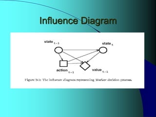
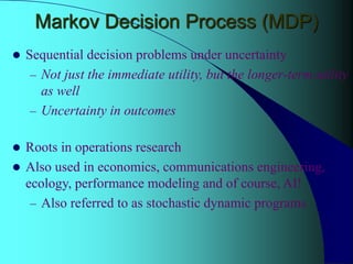
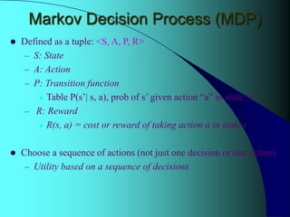
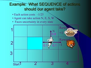
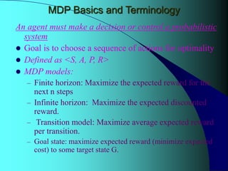
MDP Presentation
CS594
Automated Optimal Decision Making
Sohail M Yousof
Advanced Artificial Intelligence

Topic
Planning and Control in
Stochastic Domains
With
Imperfect Information

Objective
 Markov Decision Processes (Sequences of decisions)
– Introduction to MDPs
– Computing optimal policies for MDPs

Markov Decision Process (MDP)
 Sequential decision problems under uncertainty
– Not just the immediate utility, but the longer-term utility
as well
– Uncertainty in outcomes
 Roots in operations research
 Also used in economics, communications engineering,
ecology, performance modeling and of course, AI!
– Also referred to as stochastic dynamic programs

Markov Decision Process (MDP)
 Defined as a tuple: <S, A, P, R>
– S: State
– A: Action
– P: Transition function
 Table P(s’| s, a), prob of s’ given action “a” in state “s”
– R: Reward
 R(s, a) = cost or reward of taking action a in state s
 Choose a sequence of actions (not just one decision or one action)
– Utility based on a sequence of decisions

Example: What SEQUENCE of actions
should our agent take?
Reward
-1
Blocked
CELL
Reward
+1
Start1 2 3 4
1
2
3
0.8
0.1
0.1
• Each action costs –1/25
• Agent can take action N, E, S, W
• Faces uncertainty in every state
N

MDP Tuple: <S, A, P, R>
 S: State of the agent on the grid (4,3)
– Note that cell denoted by (x,y)
 A: Actions of the agent, i.e., N, E, S, W
 P: Transition function
– Table P(s’| s, a), prob of s’ given action “a” in state “s”
– E.g., P( (4,3) | (3,3), N) = 0.1
– E.g., P((3, 2) | (3,3), N) = 0.8
– (Robot movement, uncertainty of another agent’s actions,…)
 R: Reward (more comments on the reward function later)
– R( (3, 3), N) = -1/25
– R (4,1) = +1

??Terminology
• Before describing policies, lets go through some terminology
• Terminology useful throughout this set of lectures
•Policy: Complete mapping from states to actions

MDP Basics and Terminology
An agent must make a decision or control a probabilistic
system
 Goal is to choose a sequence of actions for optimality
 Defined as <S, A, P, R>
 MDP models:
– Finite horizon: Maximize the expected reward for the
next n steps
– Infinite horizon: Maximize the expected discounted
reward.
– Transition model: Maximize average expected reward
per transition.
– Goal state: maximize expected reward (minimize expected
cost) to some target state G.

???Reward Function
 According to chapter2, directly associated with state
– Denoted R(I)
– Simplifies computations seen later in algorithms presented
 Sometimes, reward is assumed associated with state,action
– R(S, A)
– We could also assume a mix of R(S,A) and R(S)
 Sometimes, reward associated with state,action,destination-state
– R(S,A,J)
– R(S,A) = S R(S,A,J) * P(J | S, A)
J

Markov Assumption
 Markov Assumption: Transition probabilities (and rewards) from
any given state depend only on the state and not on previous
history
 Where you end up after action depends only on current state
– After Russian Mathematician A. A. Markov (1856-1922)
– (He did not come up with markov decision processes
however)
– Transitions in state (1,2) do not depend on prior state (1,1)
or (1,2)

???MDP vs POMDPs
 Accessibility: Agent’s percept in any given state identify the
state that it is in, e.g., state (4,3) vs (3,3)
– Given observations, uniquely determine the state
– Hence, we will not explicitly consider observations, only states
 Inaccessibility: Agent’s percepts in any given state DO NOT
identify the state that it is in, e.g., may be (4,3) or (3,3)
– Given observations, not uniquely determine the state
– POMDP: Partially observable MDP for inaccessible environments
 We will focus on MDPs in this presentation.

MDP vs POMDP
Agent
World
States
Actions
MDP
Agent
World
Observations
Actions
SE
P
b

Stationary and Deterministic Policies
 Policy denoted by symbol 

Policy
 Policy is like a plan, but not quite
– Certainly, generated ahead of time, like a plan
 Unlike traditional plans, it is not a sequence of
actions that an agent must execute
– If there are failures in execution, agent can continue to
execute a policy
 Prescribes an action for all the states
 Maximizes expected reward, rather than just
reaching a goal state

MDP problem
 The MDP problem consists of:
– Finding the optimal control policy for all possible states;
– Finding the sequence of optimal control functions for a specific
initial state
– Finding the best control action(decision) for a specific state.

Non-Optimal Vs Optimal Policy
-1
+1
Start
1 2 3 4
1
2
3
• Choose Red policy or Yellow policy?
• Choose Red policy or Blue policy?
Which is optimal (if any)?
• Value iteration: One popular algorithm to determine optimal policy

Value Iteration: Key Idea
• Iterate: update utility of state “I” using old utility of
neighbor states “J”; given actions “A”
– U t+1 (I) = max [R(I,A) + S P(J|I,A)* U t (J)]
A J
– P(J|I,A): Probability of J if A is taken in state I
– max F(A) returns highest F(A)
– Immediate reward & longer term reward taken into
account

Value Iteration: Algorithm
• Initialize: U0 (I) = 0
• Iterate:
U t+1 (I) = max [ R(I,A) + S P(J|I,A)* U t (J) ]
A J
– Until close-enough (U t+1, Ut)
 At the end of iteration, calculate optimal policy:
Policy(I) = argmax [R(I,A) + S P(J|I,A)* U t+1 (J) ]
A J

Forward Method
for Solving MDP
Decision Tree

??Markov Chain
 Given fixed policy, you get a markov chain from the MDP
– Markov chain: Next state is dependent only on previous state
– Next state: Not dependent on action (there is only one action)
– Next state: History dependency only via the previous state
– P(S t+1 | St, S t-1, S t-2 …..) = P(S t+1 | St)
 How to evaluate the markov chain?
• Could we try simulations?
• Are there other sophisticated methods around?

Relation between
time & steps-to-go

Dynamic Construction
of the Decision Tree
 Incrémental expansion(MDP,γ, sI, є, VL, VU)
Initialize tree T with sI and ubound (sI), lbound (sI) using VL, VU;
repeat until(single action remains for sI or ubound (sI) - lbound (sI) <= є
call Improve-tree(T,MDP,γ, VL, VU)
return action with greatest lover bound as a result;
Improve-tree (T,MDP,γ, VL, VU)
if root(T) is a leaf
then expand root(T)
set bouds lbound, ubound of new leaves using VL, VU;
else for all decision subtrees T’ of T
do call Improve-tree (T,MDP,γ, VL, VU)
recompute bounds lbound(root(T)), ubound(root(T))for root(T);
when root(T) is a decision node
prune suboptimal action branches from T;
return;

Incremental expansion function:
Basic Method for the Dynamic Construction of the Decision Tree
start
MDP, γ, SI, ε, VL,
VU
OR SI)-bound(SI)
initialize leaf node of the partially
built decision tree
return
call Improve-tree(T,MDP, γ, ε, VL, VU)
Terminate

Computer Decisions
using Bound Iteration
 Incrémental expansion(MDP,γ, sI, є, VL, VU)
Initialize tree T with sI and ubound (sI), lbound (sI) using VL, VU;
repeat until(single action remains for sI or ubound (sI) - lbound (sI) <= є
call Improve-tree(T,MDP,γ, VL, VU)
return action with greatest lover bound as a result;
Improve-tree (T,MDP,γ, VL, VU)
if root(T) is a leaf
then expand root(T)
set bouds lbound, ubound of new leaves using VL, VU;
else for all decision subtrees T’ of T
do call Improve-tree (T,MDP,γ, VL, VU)
recompute bounds lbound(root(T)), ubound(root(T))for root(T);
when root(T) is a decision node
prune suboptimal action branches from T;
return;

Incremental expansion function:
Basic Method for the Dynamic Construction of the Decision Tree
start
MDP, γ, SI, ε, VL,
VU
OR (SI)-bound(SI)
initialize leaf node of the partially
built decision tree
return
call Improve-tree(T,MDP, γ, ε, VL, VU)
Terminate

If You Want to Read More
on MDPs
If You Want to Read More
on MDPs
 Book:
– Martin L. Puterman
 Markov Decision Processes
 Wiley Series in Probability
– Available on Amazon.com

RL intro

More Related Content

Similar to RL intro

Recently uploaded

RL intro