The document describes the Harris corner detector, which is used to detect interest points or corners in digital images. It works by calculating the autocorrelation matrix of an image window to determine if the window contains a corner. The autocorrelation matrix captures the gradient of the image in both the x and y directions. Corners are identified as points where both eigenvalues of the autocorrelation matrix are large, indicating a high variation in gradient in both directions. The Harris corner detector was an improvement over previous corner detectors as it considers gradient variations in all directions within a window. Examples show the Harris detector being applied to medical images to extract interest points for image registration.

1. HARRIES CORNER DETECTOR DERIVED BY LOCAL
AUTOCORRELATION FUNCTION (SURVEY)
Angu Ramesh B
Final year M.E (Medical Electronics), SXCCE, TN, INDIA
Mail: anguramesh@yahoo.in, Mobile: +918056723334
Harries operator is nothing but a corner detector in a digital image, which is
based on interest point detection. We should easily recognize the point by looking at
intensity values within an image and we can able to absolves the change of
Appearance in Neighborhood of a pixel obtained and the feature extracted with
respect to intensity pattern, so there is a possibility for incorporating either spatial and
geometrical information
In computer vision, usually we need to find matching points between different
frames of an environment. Due to know how two images relate to each other, we can
use both images to extract information of them. When we say matching points we are
referring, in a general sense, to characteristics in the scene that we can recognize easily.
We call these characteristics features such as flat regions, edges, corners (interest
points) which is shown in the figure 3.2 and figure 3.3. Corners are special than
remaining two because, since it is the intersection of two edges, it represents a point in
which the directions of these two edges change. Hence, the gradient of the image (in
both directions) have a high variation, which can be used to detect it.
3.2 EQUATION EXPLANATION
Since corners represents a variation in the gradient in the image, we will look for
this “variation”. Consider a grayscale image . We are going to sweep a
window (with displacements in the x direction and in the right
direction) and will calculate the variation of intensity.
(3.1)

2. Where:
is the window at position
is the intensity at
is the intensity at the moved window
Since we are looking for windows with corners, we are looking for windows
with a large variation in intensity. Hence, we have to maximize the equation above,
specifically the term:
(3.2)
Using Taylor expansion:
(3.3)
Expanding the equation and cancelling properly:
(3.4)
Which can be expressed in a matrix form as:
(3.5)
Let’s denote:
(3.6)

3. So, our equation now is:
(3.7)
A score is calculated for each window, to determine if it can possibly contain a
corner:
(3.8)
where:
det(M) =
trace(M) =
a window with a score greater than a certain value is considered a “corner
Figure 3.2(Corner Edge response.1) Figure 3.3(Corner Edge response.2)

4. 3.3 AUTO CORRELATION FUNCTION:
Q(x, y) = |
∑ Ix(x, y)2
w ∑ Ix(x, y).Iy(x, y)W
∑ Ix(x, y).I Y(x, y)W ∑ Iy(x, y)2
w
| = |
A B
B C
| (3.6)
W = Window function (3 x 3)
I𝑥 = Pixel Row
I𝑦 = Pixel Column
(𝑥, 𝑦) = pixel of the given window
c(x, y, Δx, Δy) = [Δx, Δy] Q(x, y) |
Δx
Δy
| (3.7)
(𝛥𝑥, 𝛥𝑦) = sifted (neighbourhood) pixel of (𝑥, 𝑦)
3.4 HARRIES OPERATOR:
ƛ1 ƛ2 = det Q(x, y) = AC − B2
; ƛ1+ƛ2 = trace Q(x, y) = (A + C) ;
H = ƛ1 ƛ2 – 0.04(ƛ1+ƛ2)2
(3.8)
det = matrix determinant
trace = sum of diagonal element
ƛ1 = curvature (intensity value) in X direction
ƛ2 = curvature (intensity value) in Y direction

5. 3.5 OVERALL BLOCK DIAGRAM OF HARRIS OPERATOR
Figure: 3.4 (Overall Block Diagram of Harris Operator)

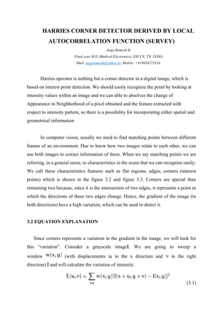
6. RESULT AND DISCUSSION
For a human, it is easier to identify a “corner”, but a mathematical detection is
required in case of algorithms. Chris Harris and Mike Stephens in 1988 improved upon
Moravec's corner detector by taking into account the differential of the corner score
with respect to direction directly instead of using shifted patches. Moravec only
considered shifts in discrete 45 degree angles whereas Harris considered all directions.
Harris detector has proved to be more accurate in distinguishing between edges
and corners. In this a circular Gaussian window is used to reduce noise and local
autocorrelation function is used for find out the correlation between the original position
and sifted position. Harris equation provides the both Eigen values of x and y direction,
when the both Eigen values are larger that’s become corner or interest points, when only
any one of Eigen values of x and y direction are larger that’s become edges, and both
Eigen values are become low, that’s become flat region. Here by the feature has been
extracted with respect to intensity pattern
In this section we are computing some test images and medical images as a X
direction [A(x,y)], Y direction [C(x,y)], Diagonal direction [B(x,y)] and also corner
detected images with their corresponding input image [I(x,y)] are shown in the
figure:3.4.

7. 4.1 OUTPUT
4.1.1 Test Image.1
Input image [I(x,y)] X direction [A(x,y)]
Figure: 4.1.1a Figure: 4.1.1b
Y direction [C(x,y)] Diagonal direction [B(x,y)]
Figure: 4.1.1c Figure: 4.1.1d
Corner detected image
Figure: 4.1.1e
Image Details: 538 X 615 X 3 No. Of Interest Points: 69

8. 4.1.2 Test Image.2
Input image [I(x,y)] X direction [A(x,y)]
Figure: 4.1.2a Figure: 4.1.2b
Y direction [C(x,y)] Diagonal direction [B(x,y)]
Figure: 4.1.2c Figure: 4.1.2d
Corner detected image
Figure: 4.1.2e
Image Details: 768 X 1024 X 3 No. Of Interest Points: 16

9. 4.1.3 Retinal Image
Input image [I(x,y)] X direction [A(x,y)]
Figure: 4.1.3a Figure: 4.1.3b
Y direction [C(x,y)] Diagonal direction [B(x,y)]
Figure: 4.1.3c Figure: 4.1.3d
Corner detected image
Figure: 4.1.3e
Image Details: 471 X 689 X 3 No. Of Interest Points: 75

10. 4.1.4 Cervical Spine Image
Input image [I(x,y)] X direction [A(x,y)]
Figure: 4.1.4a Figure: 4.1.4b
Y direction [C(x,y)] Diagonal direction [B(x,y)]
Figure: 4.1.4c Figure: 4.1.4d
Corner detected image
Figure: 4.1.4e
Image Details: 445 X 276 X 3 No. Of Interest Points: 64

11. 4.1.5 Skull Image
Input image [I(x,y)] X direction [A(x,y)]
Figure: 4.1.5a Figure: 4.1.5b
Y direction [C(x,y)] Diagonal direction [B(x,y)]
Figure: 4.1.5c Figure: 4.1.5d
Corner detected image
Figure: 4.1.5e
Image details: 556 X 541 X 3 No. of Interest points: 66

12. CONCLUSION
The image features are extracted with respect to the intensity pattern of the image
using harries corner detector which is derived by the local autocorrelation function.
Here by the system can able to achieve the spatial and geometrical information during
the similarity measurement processes
For an example, here I take 2 retinal images for registration and extracted the
features like interest points (corners) with respect to intensity pattern. Image1 has 75
interest points and image2 has 79 interest points. This points are used to labelling the
high intensity regions of the two images which can be used to find out the similarity
between the images