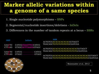
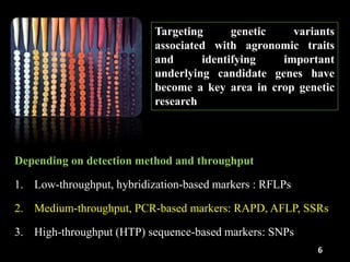
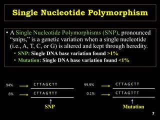
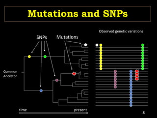
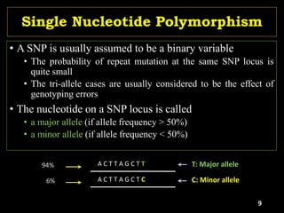
The document discusses the significance of single nucleotide polymorphisms (SNPs) in crop genetic research, emphasizing their role in accelerating crop improvement under climate change and environmental stresses. It outlines various methods for haplotype construction and the importance of tag SNPs for efficient association studies. Additionally, the text examines challenges in SNP genotype utilization and advanced strategies for haplotype mapping and inference.


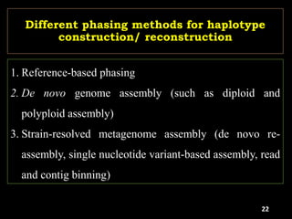
![48
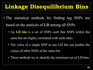
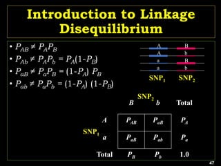
Linkage Disequilibrium
Formulas
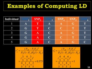
• Mathematical formulas for computing LD or Correlation:
• r2 or Δ2:
)
1
(
)
1
(
)
( 2
2
B
B
A
A
B
A
AB
P
P
P
P
P
P
P
r
)
1
(
)
1
(
)
(
)
(
Var
)
(
Var
)
,
(
Cov
2
2
2
B
B
A
A
B
A
AB
P
P
P
P
P
P
P
B
A
B
A
r
B
A
AB P
P
P
B
E
A
E
AB
E
B
A
]
[
]
[
]
[
)
,
(
Cov
)
1
(
]
[
]
[
)
(
V
2
2
2
A
A
A
A
P
P
P
P
A
E
A
E
A
ar
](https://image.slidesharecdn.com/pamb1066-240801031604-cdabdf73/85/Haplotype-mapping-and-its-application-in-Plant-Breeding-48-320.jpg)