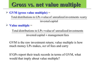
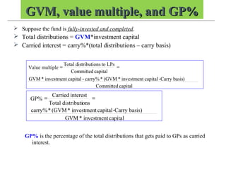
Downloaded 21 times


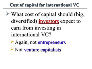
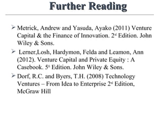
![A global multifactor model for VCA global multifactor model for VC
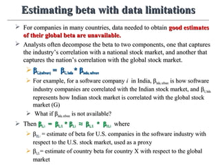
Since we almost always lack data to do this exercise for non-U.S. countries,
we use the same trick using beta decomposition into country beta (βGX) and
U.S. domestic (market, size, value, liquidity, instead of industry) beta.
Keep everything in US$.
G = global, X= country X, US = U.S.
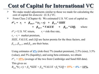
For VC investment in country X, its cost of capital, rX
VC , is:
rX
VC = rf + βmarket(G),VC(X) * (RG
m – RG
f) + βsize(G),VC(X) * SIZEG
+ βvalue(G),VC(X)* VALUEG
+ βliq(G),VC(X) * LIQG
= rf + βGX* βX
market,VC * (Rm – Rf) + βGX * βX
size,VC* SIZE
+ βGX *βX
value,VC* VALUE + βGX * βX
liq,VC* LIQ
≈ rf + βGX* βUS
market,VC * (Rm – Rf) + βGX * βUS
size,VC* SIZE
+ βGX *βUS
value,VC* VALUE + βGX * βUS
liq,VC* LIQ
= rf + βGX*
[ βUS
market,VC* (Rm – Rf) + βUS
size,VC* SIZE
+ βUS
value,VC * VALUE + βUS
liq,VC* LIQ ]
= 4% + βGX* [15% − 4% ].](https://image.slidesharecdn.com/gs503vcflecture2riskreturn310115-150210123518-conversion-gate01/85/Gs503-vcf-lecture-2-risk-return-310115-46-320.jpg)


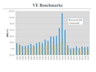
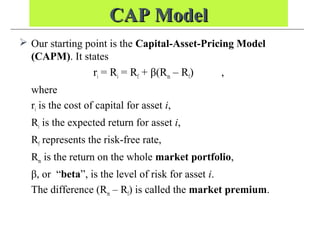
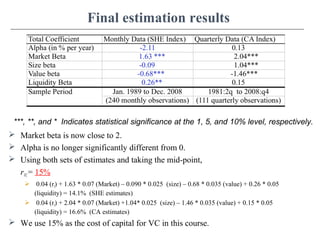
This document discusses risk and returns in the venture capital industry. It begins by defining key measures used to calculate returns, such as internal rate of return and value multiples. It then reviews data on real returns achieved by VC firms. The document also discusses estimating the cost of capital for venture capital by applying the Capital Asset Pricing Model and making adjustments for firm size, value, and illiquidity risk factors. Understanding the relationship between risk and returns is important for both venture capitalists and investors in the industry.


