Download to read offline


![2 DISCOVERY!
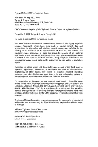
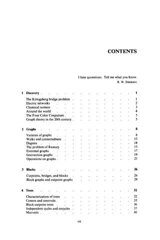
Fig. 1.1. A park in Konigsberg, 1736.
solve this problem empirically, but all attempts must be unsuccessful, for
the tremendous contribution of Euler in this case was negative, see [E5].
In proving that the problem is unsolvable, Euler replaced each land area
by a point and each bridge by a line joining the corresponding points,
thereby producing a “graph.” This graph* is shown in Fig. 1.2, where the
points are labeled to correspond to the four land areas of Fig. 1.1. Showing
that the problem is unsolvable is equivalent to showing that the graph of
Fig. 1.2 cannot be traversed in a certain way.
Rather than treating this specific situation, Euler generalized the problem
and developed a criterion for a given graph to be so traversable; namely, that
it is connected and every point is incident with an even number of lines.
While the graph in Fig. 1.2 is connected, not every point is incident with an
even number of lines.
Fig. 1.2. The graph of the Konigsberg Bridge Problem.
ELECTRIC NETWORKS
Kirchhoff [K7] developed the theory of trees in 1847 in order to solve the
system of simultaneous linear equations which give the current in each
branch and around each circuit of an electric network. Although a physicist,
he thought like a mathematician when he abstracted an electric network
* Actually, this is a “multigraph” as we shall see in Chapter 2.](https://image.slidesharecdn.com/graphtheory-181103155731/85/Graph-theory-13-320.jpg)
![CHEMICAL ISOMERS 3
with its resistances, condensers, inductances, etc., and replaced it by its
corresponding combinatorial structure consisting only of points and lines
without any indication of the type of electrical element represented by in
dividual lines. Thus, in effect, Kirchhoff replaced each electrical network
by its underlying graph and showed that it is not necessary to consider
every cycle in the graph of an electric network separately in order to solve
the system of equations. Instead, he pointed out by a simple but powerful
construction, which has since become standard procedure, that the inde
pendent cycles of a graph determined by any of its “spanning trees” will
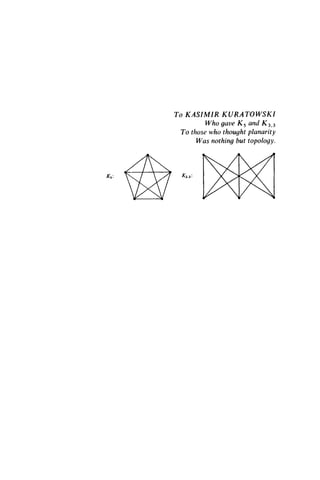
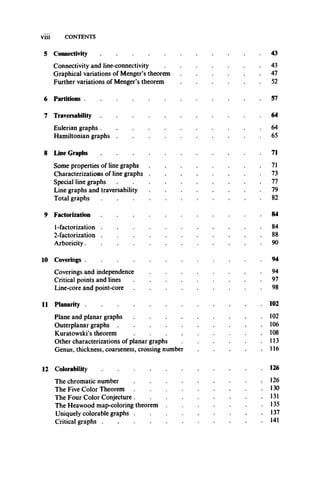
suffice. A contrived electrical network N, its underlying graph G, and a
spanning tree T are shown in Fig. 1.3.
Fig. 1.3. A network N, its underlying graph (7, and a spanning tree T.
CHEMICAL ISOMERS
In 1857, Cayley [C2] discovered the important class of graphs called trees
by considering the changes of variables in the differential calculus. Later, he
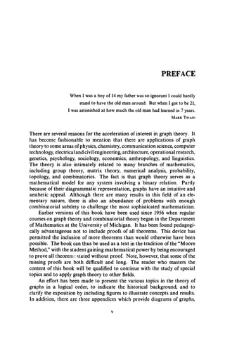
was engaged in enumerating the isomers of the saturated hydrocarbons
CnH 2n+2>with a given number n of carbon atoms, as shown in Fig. 1.4.
Of course, Cayley restated the problem abstractly: find the number
of trees with p points in which every point has degree 1 or 4. He did not
immediately succeed in solving this and so he altered the problem until he
was able to enumerate: rooted trees (in which one point is distinguished from
the others), trees, trees with points ofdegree at most 4, and finally the chemical
problem of trees in which every point has degree 1 or 4, see [C3]. Jordan
later (1869) independently discovered trees as a purely mathematical dis
cipline, and Sylvester (1882) wrote that Jordan did so “without having any
suspicion of its bearing on modem chemical doctrine,” see [K10, p. 48].](https://image.slidesharecdn.com/graphtheory-181103155731/85/Graph-theory-14-320.jpg)
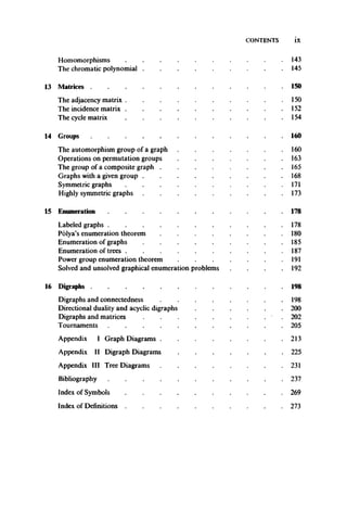
![4 DISCOVERY!
H
IH C H
IH
Methane Ethane Propane Butane
Fig. 1.4. The smallest saturated hydrocarbons.
Isobutane
AROUND THE WORLD
A game invented by Sir William Hamilton* in 1859 uses a regular solid
dodecahedron whose 20 vertices are labeled with the names of famous
cities. The player is challenged to travel “around the world” by finding a
closed circuit along the edges which passes through each vertex exactly
once. Hamilton sold his idea to a maker of games for 25 guineas; this was
a shrewd move since the game was not a financial success.
16
In graphical terms, the object of the game is to find a spanning cycle in
the graph of the dodecahedron, shown in Fig. 1.5. The points of the graph
are marked 1,2, • • •, 20 (rather than Amsterdam, Ann Arbor, Berlin, Budapest,
Dublin, Edinburgh, Jerusalem, London, Melbourne, Moscow, Novosibirsk,
New York, Paris, Peking, Prague, Rio di Janeiro, Rome, San Francisco,
Tokyo, and Warsaw), so that the existence of a spanning cycle is evident.
* See Ball and CoxeterfBCl, p. 262] for a more complete description.](https://image.slidesharecdn.com/graphtheory-181103155731/85/Graph-theory-15-320.jpg)
![GRAPH THEORY IN THE 20TH CENTURY 5
THE FOUR COLOR CONJECTURE
The most famous unsolved problem in graph theory and perhaps in all of
mathematics is the celebrated Four Color Conjecture. This remarkable
problem can be explained in five minutes by any mathematician to the so-
called man in the street. At the end of the explanation, both will understand
the problem, but neither will be able to solve it.
The following quotation from the definitive historical article by May
[M5] states the Four Color Conjecture and describes its role :
[The conjecture states that] any map on a plane or the surface of a sphere can be
colored with only four colors so that no two adjacent countries have the same
color. Each country must consist of a single connected region, and adjacent
countries are those having a boundary line (not merely a single point) in common.
The conjecture has acted as a catalyst in the branch of mathematics known as
combinatorial topology and is closely related to the currently fashionable field of
graph theory. More than half a century of work by many (some say all) mathe
maticians has yielded proofs for special cases . .. The consensus is that the con
jecture is correct but unlikely to be proved in general. It seems destined to retain
for some time the distinction of being both the simplest and most fascinating
unsolved problem of mathematics.
The Four Color Conjecture has an interesting history, but its origin
remains somewhat vague. There have been reports that Mobius was familiar
with this problem in 1840, but it is only definite that the problem was com
municated to De Morgan by Guthrie about 1850. The first of many erroneous
“proofs” of the conjecture was given in 1879 by Kempe [K6]. An error was
found in 1890 by Heawood [H38] who showed, however, that the conjecture
becomes true when “four” is replaced by “five.” A counterexample, if ever
found, will necessarily be extremely large and complicated, for the con
jecture was proved most recently by Ore and Stemple [OS1] for all maps
with fewer than 40 countries.
The Four Color Conjecture is a problem in graph theory because every
map yields a graph in which the countries (including the exterior region) are
the points, and two points are joined by a line whenever the corresponding
countries are adjacent. Such a graph obviously can be drawn in the plane
without intersecting lines. Thus, if it is possible to color the points of every
planar graph with four or fewer colors so that adjacent points have different
colors, then the Four Color Conjecture will have been proved.
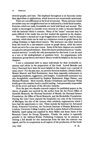
GRAPH THEORY IN THE 20th CENTURY
The psychologist Lewin [L2] proposed in 1936 that the “fife space” of an
individual be represented by a planar map.* In such a map, the regions
would represent the various activities of a person, such as his work environ-
* Lewin used only planar maps because he always drew his figures in the plane.](https://image.slidesharecdn.com/graphtheory-181103155731/85/Graph-theory-16-320.jpg)
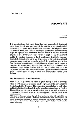
![6 DISCOVERY!
Fig. 1.6. A map and its corresponding graph.
ment, his home, and his hobbies. It was pointed out that Lewin was actually
dealing with graphs, as indicated by Fig. 1.6. This viewpoint led the psy
chologists at the Research Center for Group Dynamics to another psycho
logical interpretation of a graph, in which people are represented by points
and interpersonal relations by lines. Such relations include love, hate,
communication, and power. In fact, it was precisely this approach which led
the author to a personal discovery of graph theory, aided and abetted by
psychologists L. Festinger and D. Cartwright.
The world of theoretical physics discovered graph theory for its own
purposes more than once. In the study of statistical mechanics by Uhlenbeck
[U l], the points stand for molecules and two adjacent points indicate
nearest neighbor interaction of some physical kind, for example, magnetic
attraction or repulsion. In a similar interpretation by Lee and Yang [LY1],
the points stand for small cubes in euclidean space, where each cube may or
may not be occupied by a molecule. Then two points are adjacent whenever
both spaces are occupied. Another aspect of physics employs graph theory
rather as a pictorial device. Feynmann [F3] proposed the diagram in
which the points represent physical particles and the lines represent paths of
the particles after collisions.
The study of Markov chains in probability theory (see, for example,
Feller [F2, p. 340]) involves directed graphs in the sense that events are
represented by points, and a directed line from one point to another indicates
a positive probability of direct succession of these two events. This is made
explicit in the book [HNC1, p. 371] in which a Markov chain is defined as a
network with the sum of the values of the directed lines from each point
equal to 1. A similar representation of a directed graph arises in that part
of numerical analysis involving matrix inversion and the calculation of
eigenvalues. Examples are given by Varga [V2, p. 48]. A square matrix is
given, preferably “sparse,” and a directed graph is associated with it in the
following way. The points denote the index of the rows and columns of the](https://image.slidesharecdn.com/graphtheory-181103155731/85/Graph-theory-17-320.jpg)
![GRAPH THEORY IN THE 20TH CENTURY 7
given matrix, and there is a directed line from point / to point j whenever
the i, j entry of the matrix is nonzero. The similarity between this approach
and that for Markov chains is immediate.
The rapidly growing fields of linear programming and operational
research have also made use of a graph theoretic approach by the study of
flows in networks. The books by Ford and Fulkerson [FF2], Vajda [VI]
and Berge and Ghouila-Houri [BG2] involve graph theory in this way. The
points of a graph indicate physical locations where certain goods may be
stored or shipped, and a directed line from one place to another, together
with a positive number assigned to this line, stands for a channel for the
transmission of goods and a capacity giving the maximum possible quantity
which can be shipped at one time.
Within pure mathematics, graph theory is studied in the pioneering
book on topology by Veblen [V3, pp. 1-35]. A simplicial complex (or
briefly a complex) is defined to consist of a collection V of “points” together
with a prescribed collection S of nonempty subsets of V, called “simplexes,”
satisfying the following two conditions.
1. Every point is a simplex.
2. Every nonempty subset of a simplex is also a simplex.
The dimension ofa simplex is one less than the number of points in it;that
of a complex is the maximum dimension of any simplex in it. In these terms,
a graph may be defined as a complex of dimension 1 or 0. We call a 1-
dimensional simplex a line, and note that a complex is 0-dimensional if and
only if it consists of a collection of points, but no lines or other higher
dimensional simplexes. Aside from these “totally disconnected” graphs,
every graph is a 1-dimensional complex. It is for this reason that the subtitle
of the first book ever written on graph theory [K10] is “Kombinatorische
Topologie der Streckenkomplexe.”
It is precisely because of the traditional use of the words point and line
as undefined terms in axiom systems for geometric structures that we have
chosen to use this terminology. Whenever we are speaking of “geometric”
simplicial complexes as subsets of a euclidean space, as opposed to the
abstract complexes defined above, we shall then use the words vertex and
edge. Terminological questions will now be pursued in Chapter 2, together
with some of the basic concepts and elementary theorems of graph theory.](https://image.slidesharecdn.com/graphtheory-181103155731/85/Graph-theory-18-320.jpg)
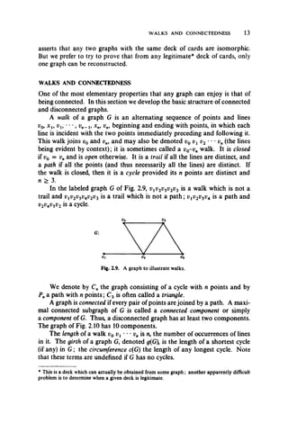
![12 GRAPHS
vt
G—v2v3:
Vs
G+v3u5:
04 l>3
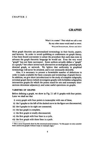
Fig. 2.7. A graph plus or minus a specific point or line.
smallest supergraph of G containing the line v^j, These concepts are illus
trated in Fig. 2.7.
There are certain graphs for which the result of deleting a point or line,
or adding a line, is independent of the particular point or line selected. If
this is so for a graph G, we denote the result accordingly by G — p, G - x,
or G + x ; see Fig. 2.8.
It was suggested by Ulam [U2, p. 29] in the following conjecture that
the collection of subgraphs G — pf of G gives quite a bit of information
about G itself.
Fig. 2.8. A graph plus or minus a point or line.
Ulam's Conjecture * Let G have p points pf and H have p points uf, with
p > 3. If for each i, the subgraphs G, = G - p, and tf, = H - u* are
isomorphic, then the graphs G and H are isomorphic.
There is an alternative point of view to this conjecture [H29]. Draw
each of the p unlabeled graphs G — p, on a 3 x 5 card. The conjecture then
states that any graph from which these subgraphs can be obtained by de
leting one point at a time is isomorphic to G. Thus Ulam’s conjecture
* The reader is urged not to try to settle this conjecture since it appears to be rather difficult.](https://image.slidesharecdn.com/graphtheory-181103155731/85/Graph-theory-23-320.jpg)
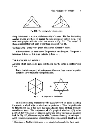
![14 GRAPHS
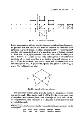
Fig. 2.10. A graph with 10 components.
The distance d(u, p) between two points u and v in G is thelengthof a
shortest path joining them if any; otherwise d(u, p) = oo. Ina connected
graph, distance is a metric; that is, for all points w, p, and w,
1. d(u, v) > 0, with d(u, p) = 0 if and only if u = p.
2. p) = d(p, w).
3. d(n, p) + d(v, w) > d(u, w).
A shortest w-p path is often called a geodesic. The diameter d(G) of a
connected graph G is the length of any longest geodesic. The graph G of
Fig. 2.9 has girth g = 3, circumference c = 4, and diameter d = 2.
The square G2 of a graph G has F(G2) = F(G) with w, p adjacent in G2
whenever d(u, v) < 2 in G. The powers G3, G4, • •of G are defined similarly.
DEGREES
The degree* of a point p, in graph G, denoted or deg pf, is the number of
lines incident with vt. Since every line isincident with two points,it contrib
utes 2 to the sum of the degrees of the points. We thus have a result, due to
Euler [E6], which was the first theorem of graph theory!
Theorem Z1 The sum of the degrees of the points of a graph G is twice
the number of lines,
£ deg = 2q. (2.1)
Corollary 2.1(a) In any graph, the number of points of odd degree is even.t
In a (p, q) graph, 0 < deg v < p — 1 for every point v. The minimum
degree among the points of G is denoted min deg G or <5(G) while A(G) =
max deg G is the largest such number. If 8(G) = A(G) = r, then all points
have the same degree and G is called regular of degree r. We then speak
of the degree of G and write deg G = r.
A regular graph of degree 0 has no lines at all. If G is regular of degree
1, then every component contains exactly one line; if it is regular of degree 2,
* Sometimes called valency.
t The reader is reminded (see the Preface) that not all theorems are proved in the text.](https://image.slidesharecdn.com/graphtheory-181103155731/85/Graph-theory-25-320.jpg)
![16 GRAPHS
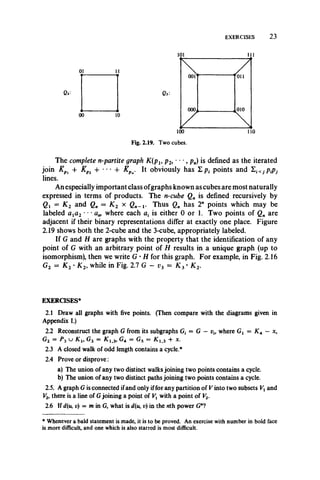
Fig. 2.13. The smallest nontrivial self-complementary graphs.
The complete graph K p has every pair of its p points* adjacent. Thus
Kp has (5) lines and is regular of degree p — 1. As we have seen, K 3 is
called a triangle. The graphs Kp are totally disconnected, and are regular
of degree 0.
In these terms, the puzzle may be reformulated.
Theorem 2.2 For any graph G with six points, G or G contains a triangle.
Proof. Let v be a point of a graph G with six points. Since v is adjacent
either in G or in G to the other five points of G, we can assume without
loss of generality that there are three points uu u2, w3 adjacent to v in G.
If any two of these points are adjacent, then they are two points of a triangle
whose third point is v. If no two of them are adjacent in G, then uu n2, and
u3 are the points of a triangle in G.
The result of Theorem 2.2 suggests the general question: What is the
smallest integer r(ro, n) such that every graph with r(m, n) points contains
K mor K„1
The values r(m, n) are called Ramsey numbersf Of course r(m, n) =
r(n, m). The determination of the Ramsey numbers is an unsolved problem,
although a simple bound due to Erdos and Szekeres [ESI] is known.
( m + n — 2
* ”•">4 -"-I )
This problem arose from a theorem of Ramsey. An infinite graph% has
an infinite point set and no loops or multiple lines. Ramsey [R2] proved
(in the language of set theory) that every infinite graph contains K0 mutually
adjacent points or K0 mutually nonadjacent points.
All known Ramsey numbers are given in Table 2.1, in accordance with
the review article by Graver and Yakel [GY1].
* Since V is not empty, p > 1. Some authors admit the “empty graph” (which we would
denote K0 if it existed) and are then faced with handling its properties and specifying that
certain theorems hold only for nonempty graphs, but we consider such a concept pointless.
t After Frank Ramsey, late brother of the present Archbishop of Canterbury. For a proof
that r(m, n) exists for all positive integers mand n, see for example Hall [H7, p. 57].
t Note that by definition, an infinite graph is not a graph. A review article on infinite graphs
was written by Nash-Williams [N3].](https://image.slidesharecdn.com/graphtheory-181103155731/85/Graph-theory-27-320.jpg)
![EXTREMAL GRAPHS 17
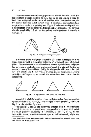
Table 2.1
RAMSEY NUMBERS
«m 2 3 4 5 6 7
2 2 3 4 5 6 7
3 3 6 9 14 18 23
4 4 9 18
EXTREMAL GRAPHS
The following famous theorem of Turan [T3] is the forerunner of the field
of extremal graph theory, see [E3]. As usual, let [r] be the greatest integer
not exceeding the real number r, and {r} = —[ —r], the smallest integer
not less than r.
Theorem 2.3 The maximum number of lines among all p point graphs with no
triangles is [p2/4].
Proof. The statement is obvious for small values of p. An inductive proof
may be given separately for odd p and for even p ; we present only the latter.
Suppose the statement is true for all even p < 2n. We then prove it for
p = In + 2. Thus, let G be a graph with p = In + 2 points and no triangles.
Since G is not totally disconnected, there are adjacent points u and v. The
subgraph G' = G — {u, v} has 2n points and no triangles, so that by the
inductive hypotheses G' has at most [4n2/4] = n2 lines. How many more
lines can G have? There can be no point w such that u and v are both adjacent
to w, for then u, v9and w would be points of a triangle in G. Thus if u is
adjacent to k points of G', v can be adjacent to at most 2n — k points. Then
G has at most
n2 + k 4- (2n — k) + 1 = n2 + In -f 1 = p2j4 = [p2/4] lines.
To complete the proof, we must show that for all even p, there exists a
(p, p2/4) graph with no triangles. Such a graph is formed as follows: Take
two sets Vx and V2 of p/2 points each and join each point of Vt with each
point of V2. For p = 6, this is the graph G{ of Fig. 2.5.
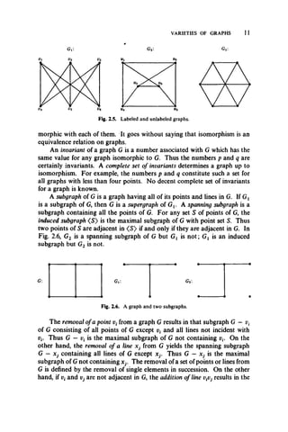
A bigraph (or bipartite graph*) G is a graph whose point set V can be
partitioned into two subsets Vl and V2 such that every line of Gjoins Vx with
V2. For example, the graph of Fig. 2.14(a) can be redrawn in the form of
Fig. 2.14(b) to display the fact that it is a bigraph.
If G contains every line joining Vxand V2, then G is a complete bigraph. If
Vx and V2 have m and n points, we write G = Kmn = K(m, n). A starf is a
* Also called bicolorable graph, pair graph, even graph, and other things,
t When n —3, Hoffman [H43] calls Kl na “claw”; Erdos and Renyi [ER1], a “cherry.”](https://image.slidesharecdn.com/graphtheory-181103155731/85/Graph-theory-28-320.jpg)
![18 GRAPHS
(a) (b)
Fig. 2.14. A bigraph.
complete bigraph K ln . Clearly K mn has mn lines. Thus, if p is even,
K(p/2, p/2) has p2/4 lines, while if p is odd, K([p/2], {p/2}) has [p/2] {p/2} =
[p2/4] lines. That all such graphs have no triangles follows from a theorem
of Konig [K10, p. 170].
Theorem 2.4 A graph is bipartite if and only if all its cycles are even.
Proof. If G is a bigraph, then its point set V can be partitioned into two sets
Vx and V2 so that every line of G joins a point of Vx with a point of V2. Thus
every cycle vxv2 • • • vnv1 in G necessarily has its oddly subscripted points
in Vu say, and the others in V2, so that its length n is even.
For the converse, we assume, without loss of generality, that G is
connected (for otherwise we can consider the components of G separately).
Take any point V, and let Vx consist of vt and all points at even distance
from vu while V2 = V — Vx. Since all the cycles of G are even, every line
of G joins a point of Vx with a point of V2. For suppose there is a line uv
joining two points of Vt. Then the union of geodesics from vx to v and from
vx to u together with the line uv contains an odd cycle, a contradiction.
Theorem 2.3 is the first instance of a problem in “extremal graph theory” :
for a given graph H, find ex (p, H the maximum number of lines that a
graph with p points can have without containing the forbidden subgraph H.
Thus Theorem 2.3 states that ex (p, K 3) = [p2/4]. Some other results [E3]
in extremal graph theory are:
Turan [T3] generalized his Theorem 2.3 by determining the values of
ex (p, Kn) for all n < p,
ex (p, Cp) = 1 + (p - 1)(p - 2)/2,
ex (p, K a - x) = [p2/4],
ex (p, K 1i3 + x) = [p2/4].
(2.3)
(2.4)
(2.5)
(2.6)](https://image.slidesharecdn.com/graphtheory-181103155731/85/Graph-theory-29-320.jpg)
![INTERSECTION GRAPHS 19
where p = r mod (n - 1) and 0 < r < n — 1. A new proof of this result
was given by Motzkin and Straus [M SI].
It is also known that every (2n, n2 + 1) graph contains n triangles, every
(p, 3p — 5) graph contains two disjoint cycles for p > 6, and every
(3n, 3n2 4- 1) graph contains n2 cycles of length 4.
INTERSECTION GRAPHS
Let S be a set and F = {Sx, ■• • , Sp}a nonempty family of distinct nonempty
subsets of S whose union is S. The intersection graph of F is denoted Q(F)
and defined by F(Q(F)) = F, with S, and S, adjacent whenever i ^ j and
S. n # 0. Then a graph G is an intersection graph on S if there exists a
family F of subsets of S for which G = Q(F). An early result [M4] on inter
section graphs is now stated.
Theorem 2.5 Every graph is an intersection graph.
Proof. For each point v( of G, let S, be the union of {pj with the set of lines
incident with i Then it is immediate that G is isomorphic with S1(F) where
F = {SJ.
In view of this theorem, we can meaningfully define another invariant.
The intersection number co(G) of a given graph G is the minimum number of
elements in a set S such that G is an intersection graph on S.
Corollary 2.5(a) If G is connected and p > 3, then co(G) < q.
Proof. In this case, the points can be omitted from the sets St used in the
proof of the theorem, so that S = X(G).
Corollary 2.5(b) If G has p0 isolated points and no K 2 components, then
a)(G) < q + p0.
The next result tells when the upper bound in Corollary 2.5(a) is attained.
Theorem 2.6 Let G be a connected graph with p > 3 points. Then co(G) = q
if and only if G has no triangles.
Proof. We first prove the sufficiency. In view of Corollary 2.5(a), it is only
necessary to show that co(G) > q for any connected G with at least 4 points
having no triangles. By definition of the intersection number, G is isomorphic
with an intersection graph Cl(F) on a set S with S = cu(G). For each point
vt of G, let St be the corresponding set. Because G has no triangles, no
element of S can belong to more than two of the sets and S, n Sj ^ 0
if and only if i i s a line of G. Thus we can form a 1-1 correspondence
between the lines of G and those elements of S which belong to exactly two
sets Therefore co(G) = S > q so that cu(G) = q.
To prove the necessity, let w(G) = q and assume that G has a triangle.
Then let Gj be a maximal triangle-free spanning subgraph of G. By the
preceding paragraph, a^G^ = qx ~ ^(G ^l. Suppose that Gx = Q(F),](https://image.slidesharecdn.com/graphtheory-181103155731/85/Graph-theory-30-320.jpg)
![2 0 GRAPHS
where F is a family of subsets of some set S with cardinality qt. Let x be a line
of G not in Gj and consider G2 = Gx + x. Since Gt is maximal triangle-free,
G2 must have some triangle, say ulu2w3, where x = uxu3. Denote by
S l9 S2, S3 the subsets of S corresponding to ul9 u2, u3. Now if u2 is adjacent
to only uv and u3 in Gu replace S2 by a singleton chosen from S t n S2, and
add that element to S3. Otherwise, replace S3 by the union of S3 and any
element in S t n S2. In either case this gives a family F' of distinct subsets
of S such that G2 = G(F'). Thus co(G2) < qt while X(G2) = q { + 1. If
G2 £ G, there is nothing to prove. But if G2 ^ G, then let
X(G) - X(G2) = q0.
It follows that G is an intersection graph on a set with qt + q0 elements.
However, qx + q0 = q - 1. Thus co(G) < q, completing the proof.
The intersection number of a graph had previously been studied by
Erdos, Goodman, and Posa [EGP1]. They obtained the best possible upper
bound for the intersection number of a graph with a given number of
points.
Theorem 2.7 For any graph G with p > 4 points, cu(G) < [p2/4].
Their proof is essentially the same as that of Theorem 2.3.
There is an intersection graph associated with every graph which depends
on its complete subgraphs. A clique of a graph is a maximal complete
subgraph. The clique graph of a given graph G is the intersection graph of
the family of cliques of G. For example, the graph G of Fig. 2.15 obviously
has K 4 as its clique graph. However, it is not true that every graph is the
clique graph of some graph, for Hamelink [H9] has shown that the same
graph G is a counterexample! F. Roberts and J. Spencer have just char
acterized clique graphs:
Theorem 2.8 A graph G is a clique graph if and only if it contains a family
F of complete subgraphs, whose union is G, such that whenever every pair
of such complete graphs in some subfamily F ' have a nonempty inter
section, the intersection of all the members of F' is not empty.
Fig. 2.15. A graph and its clique graph.
Excursion
A special class of intersection graphs was discovered in the field of genetics
by Benzer [B9] when he suggested that a string of genes representing a](https://image.slidesharecdn.com/graphtheory-181103155731/85/Graph-theory-31-320.jpg)
![OPERATIONS ON GRAPHS 21
bacterial chromosome be regarded as a closed interval on the real line.
Hajos [H2] independently proposed that a graph can be associated with
every finite family F of intervals Si9which in terms of intersection graphs, is
precisely Q(F). By an interval graph is meant one which is isomorphic to
some graph Q(F), where F is a family of intervals. Interval graphs have been
characterized by Boland and Lekkerkerker [BL2] and by Gilmore and
Hoffman [GH2].
Fig. 2.16. The union andjoin of two graphs.
OPERATIONS ON GRAPHS
It is rather convenient to be able to express the structure of a given graph
in terms of smaller and simpler graphs. It is also of value to have notational
abbreviations for graphs which occur frequently. We have already introduced
the complete graph K p and its complement Xp, the cycle C„, the path Pn,
and the complete bigraph K mn.
Throughout this section, graphs Gx and G2 have disjoint point sets Vx
and V2 and line sets X x and X 2 respectively. Their union* G = Gx u G2 has,
as expected, V = Vx u V2 and X = X x u X 2- Their join defined by
Zykov [Z l] is denoted Gx + G2 and consists of Gx u G2 and all lines
joining Vx with V2. In particular, K mn = Km + Kn. These operations are
illustrated in Fig. 2.16 with Gx = K 2 = P2 and G2 = K X2 = P 3.
For any connected graph G, we write nG for the graph with n components
each isomorphic with G. Then every graph can be written as in [HP14] in
the form U nfii with Gf different from Gj for i ^ j . For example, the
disconnected graph of Fig. 2.10 is 4K x u 3K 2 u 2K Z u K l 2.
There are several operations on Gx and G2 which result in a graph G
whose set of points is the cartesian product Vx x V2. These include the
product (or cartesian product, see Sabidussi [S5]), and the composition
[H21] (or lexicographic product, see Sabidussi [S6]). Other operationsf of
this form are developed in Harary and Wilcox [HW1].
*Ofcourse the union of two graphs which are not disjoint is also defined this way.
t These include the tensor product (Weichsel [W6J, MeAndrew [M7], Harary and Trauth
[HT1], Brualdi[Bl7|), and other kinds of product defined in Berge[B12, p. 23], 0re[05, p. 35],
and Teh and YapfTYl].](https://image.slidesharecdn.com/graphtheory-181103155731/85/Graph-theory-32-320.jpg)
![2 2 GRAPHS
G,:
(« 1. “ 2) (M l, v 2) ( u u W2)
U-x v2 w2
G2: • ■" « GxX G2*.
( » i. m2) (© ,, v 2) (v u w 2)
Fig. 2.17. The product of two graphs.
(Mi, u2) (M l, l>2) (M l, w2)
Fig. 2.18. Two compositions of graphs.
To define the product Gt x G2, consider any two points u = {ul9 u2)
and v = (vl9 v2) in V = Vt x F2. Then u and t>are adjacent in Gx x G2
whenever [ux = vt and u2 adj t?2] or [w2 = v2 and ux adj t^]. The product
of Gx = P2 and G2 = P3 is shown in Fig. 2.17.
The composition G = G ^ G J also has V = Vx x F2 as its point set,
and w = (ul9 u2) is adjacent with v = (i?t, v2) whenever [ux adj i?j] or
[ux = and u2 adj p2]. For the graphs Gx and G2 of Fig. 2.17, both com
positions Gt[G2] and G ^ G ^ , which are obviously not isomorphic, are
shown in Fig. 2.18.
If Gt and G2are (pu qx) and (p2, q2) graphs respectively, then for each of
the above operations, one can calculate the number of points and lines in the
resulting graph, as shown in the following table.
Table 2.2
BINARY OPERATIONS ON GRAPHS
Operation Number of points Number of lines
Union Gi u G2 Pi + P2 <Ii + ?2
Join Gi + G2 Pi + P2 <h + 42 + P1P2
Product Gj x G2 P1P2 P1Q2 + P2Q1
Composition G,[G2] P1P2 Pl<l2 + Pill](https://image.slidesharecdn.com/graphtheory-181103155731/85/Graph-theory-33-320.jpg)
![2 4 GRAPHS
2.7 A graph H is a square root of G if H2 = G. A graph Gwith p points has a square
root if and only if it contains p complete subgraphs G, such that
1. u. eG,,
2. v{e Gj if and only if Vj e G,,
3. each line of G is in some G,. (Mukhopadhyay [M l8])
2.8 A finite metric space (5, d) is isomorphic to the distance space of some graph if
and only if
1. The distance between any two points of S is an integer,
2. If d(u, d) > 2, then there is a third point w such that d(u, w) + d(w, v) ~ d(u, v).
(Kay and Chartrand [KC1])
2.9 In a connected graph any two longest paths have a point in common.
2.10 It is not true that in every connected graph all longest paths have a point in
common. Verify that Fig. 2.20 demonstrates this. (Walther [W4])
2.11 Every graph with diameter d and girth 2d + 1 is regular. (Singleton [SI3])
2.12 Let G be a (p, q) graph all of whose points have degree k or k + 1. If G has
pk > 0 points of degree k and pk+xpoints of degree k + 1, then pk = (k + l)p —2q.
2.13 Construct a cubic graph with In points (n > 3) having no triangles.
2.14 If G has p points and <5(G) > (p — l)/2, then Gis connected.
2.15 If G is not connected then G is.
2.16 Every self-complementary graph has 4n or 4n + 1 points.
2.17 Draw any four of the ten self-complementary graphs with eight points.
2.18 Every nontrivial self-complementary graph has diameter 2 or 3.
(Ringel [R ll], Sachs [S8])
2.19 The Ramsey numbers satisfy the recurrence relation,
r(m, w) < r(m — 1, n) + r(mfn — 1). (Erdos and Szekeres [ESI])
2.20 Find the maximum number of lines in a graph with p points and no even cycles.](https://image.slidesharecdn.com/graphtheory-181103155731/85/Graph-theory-35-320.jpg)
![EXERCISES 25
2.21 Find the extremal graphs which do not contain K4.
2.22 Every (p, p 4- 4) graph contains two line-disjoint cycles.
(Turan [T3])
(Erdos [E3])
2.23 The only (p, [p2/4]) graph with no triangles is K([p/2], {p/2}).
2.24 Prove or disprove:The only graph on ppoints with maximum intersection number
is K([p/2], {p/2})-
2.25 The smallest graph having every line in at least two triangles but some line in no
126 Determine co(Kp), co(Cn 4- K x w(Cn + C„), and a)(Cn).
2.27 Prove or disprove:
a) The number of cliques of Gdoes not exceed co(G).
b) The number of cliques of G is not less than co(G).
128 Prove that the maximum number of cliques in a graphwith p points where
p - 4 = 3r + s, s - 0, 1 or 2, is 22_53r+s. (Moon and Moser[MM1])
2.29 A cycle of length 4 cannot be an induced subgraph of an interval graph.
2.30 Let s(n) denote the maximum number of points in the w-cube which induce a
cycle. Verify the following table:
2.31 Prove or disprove: If Gt and G2 are regular, then so is
a) Gj + G2. b) Gx x G2. c) Gj[G2].
2.32 Prove or disprove: If Gt and G2 are bipartite, then so is
a) Gj 4- G2. b) Gx x G2. c) Gt[G2].
2.33 Prove or disprove:
a) G1 4- G2 = Gx 4- G2. b) Gx x G2 = Gx x G2. c) Gj[G2] = C72[G2].
134 a) Calculate the number of cycles in the graphs (a) C„ 4- K x, (b) Kp1(c) Kmn.
(Harary and Manvel [HM1])
b) What is the maximum number of line-disjoint cycles in each of these three
graphs? (Chartrand, Geller, and Hedetniemi [CGH2])
2.35 The conjunction Gx a G2 has Vx x V2as its point set and u = (uu u2)is adjacent
to v = (vx, v2) whenever uxadj vxand u2adj v2. Then when Gxand G2 are connected,
Gj x G2 = G, a G2 if and only ifG t s G2 ^ C2m+X. (Miller [M il])
2.36 The conjunction Gj a G2 of two connected graphs is connected if and only if
Gxor G2 has an odd cycle.
*137 There exists a regular graph of degree r with r2 4- 1 points and diameter 2 only
for r = 2, 3, 7, and possibly 57. (Hoffman and Singleton [HS1])
*138 A graph G with p — 2n has the property that for every set S of n points, the
induced subgraphs <S> and (V —S) are isomorphic if and only if G is one of the
following: Kln, Kn x K2, 2Kn, 2C4, and their complements.
K4 is the octahedron K2 4- C4. (J. Cameron and A. R. Meetham)
n 2 3 4 5
s(n) 4 6 8 14 (Danzer and Klee [DK1])
(Kelly and Merriell [KM1])](https://image.slidesharecdn.com/graphtheory-181103155731/85/Graph-theory-36-320.jpg)
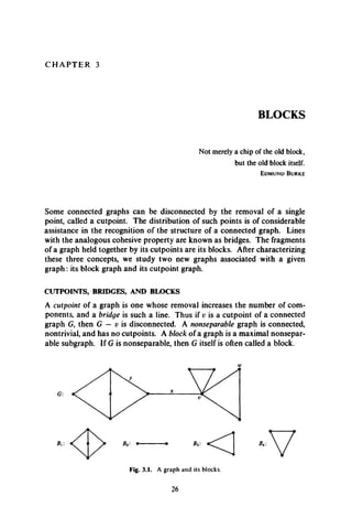
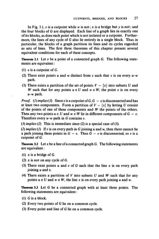
![3 0 BLOCKS
the other hand, to obtain a graph whose points correspond to the cutpoints
of G, we can take the sets S, to be the union of all blocks which contain the
cutpoint v(. The resulting intersection graph Q(F) is called the cutpoint
graph, C(G). Thus two points of C(G) are adjacent if the cutpoints of G to
which they correspond lie on a common block. Note that C(G) is defined
only for graphs G which have at least one cutpoint. Figure 3.3 illustrates
these concepts, which were introduced in [H28].
Theorem 3.5 A graph H is the block graph of some graph if and only if every
block of H is complete.
Proof. Let H = B(G), and assume there is a block ff, of H which is not
complete. Then there are two points in ff, which are nonadjacent and lie on
a shortest common cycle Z of length at least 4. But the union of the
blocks of G corresponding to the points of if, which lie on Z is then connected
and has no cutpoint, so it is itself contained in a block, contradicting the
maximality property of a block of a graph.
On the other hand, let if be a given graph in which every block is com
plete. Form B(ff), and then form a new graph G by adding to each point if,
of B{H) a number of endlines equal to the number of points of the block if,
which are not cutpoints of if. Then it is easy to see that B(G) is isomorphic
to if.
Clearly the same criterion also characterizes cutpoint graphs.
EXERCISES
3.1 What is the maximum number of cutpoints in a graph with p points?
3.2 A cubic graph has a cutpoint if and only if it has a bridge.
3.3 The smallest number of points in a cubic graph with a bridge is 10.
3.4 If v is a cutpoint of G, then v is not a cutpoint of the complement G.
(Harary [H I5])
3.5 A point v of G is a cutpoint if and only if there are points u and w adjacent to
t; such that v is on every u-w path.
3.6 Prove or disprove: A connected graph G with p > 3 is a block if and only if
given any two points and one line, there is a path joining the points which does not
contain the line.
3.7 A connected graph with at least two lines is a block ifand only if any two adjacent
lines lie on a cycle.
3.8 Let G be a connected graph with at least three points. The following statements
are equivalent:
1. G has no bridges.
2. Every two points of G lie on a common closed trail.
3. Every point and line of G lie on a common closed trail.](https://image.slidesharecdn.com/graphtheory-181103155731/85/Graph-theory-41-320.jpg)
![EXERCISES 31
4. Every two lines of Glie on a common closed trail.
5. For every pair of points and every line of G, there is a trail joining the points
which contains the line.
6. For every pair of points and every line of G, there is a path joining the points
which does not contain the line.
7. For every three points there is a trail joining any two which contains the third.
3.9 If G is a block with S > 3, then there is a point v such that G — v is also a block.
(A. Kaugars)
3.10 The square of every nontrivial connected graph is a block.
3.11 If G is a connected graph with at least one cutpoint, then B(B(G)) is isomorphic
to C(G).
3.12 Let b(v) be the number of blocks to which point v belongs in a connected graph
G. Then the number of blocks of G is given by
b(G) - 1 = 1 [b(v) - 1]. (Harary [H22])
3.13 Let c(B) be the number of cutpoints of a connected graph G which are points of
the block B. Then the number of cutpoints of G is given by
c(G) - 1 = 1 [c(B) - 1]. (Gallai [G3])
3.14 A block G is line-critical if every subgraph G —x is not a block. A diagonal of G
is a line joining two points of a cycle not containing it. Let G be a line-critical block
with p > 4.
a) G has no diagonals.
b) G contains no triangles.
c) p < q ^ 2p - 4.
d) The removal of all points of degree 2 results in a disconnected graph, provided
G is not a cycle. (Plummer [P4])](https://image.slidesharecdn.com/graphtheory-181103155731/85/Graph-theory-42-320.jpg)
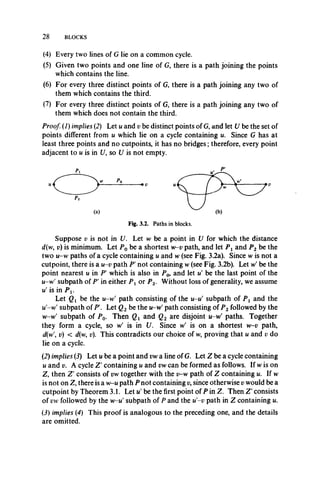
![CENTERS AND CENTROIDS 35
CENTERS AND CENTROIDS
The eccentricity e(v) of a point v in a connected graph G is max d(u, i;) for all
u in G. The radius r(G) is the minimum eccentricity of the points. Note that
the maximum eccentricity is the diameter. A point v is a central point if
e(v) = r(G), and the center of G is the set of all central points.
In the tree of Fig. 4.2, the eccentricity of each point is shown. This tree
has diameter 7, radius 4, and the center consists of the two points u and v9
each with minimum eccentricity 4. The fact that u and v are adjacent
illustrates a result discovered by Jordan* and independently by Sylvester;see
Konig [K10, p. 64].
Theorem 4.2 Every tree has a center consisting of either one point or two
adjacent points.
Proof. The result is obvious for the trees K x and K 2. We show that any
other tree T has the same central points as the tree T obtained by removing
all endpoints of T. Clearly, the maximum of the distances from a given point
u of T to any other point v of T will occur only when v is an endpoint.
Thus, the eccentricity of each point in T will be exactly one less than the
eccentricity of the same point in T. Hence the points of T which possess
minimum eccentricity in T are the same points having minimum eccentricity
in T', that is, T and T have the same center. If the process of removing
endpoints is repeated, we obtain successive trees having the same center
as T. Since T is finite, we eventually obtain a tree which is either K x or K 2.
In either case all points of this ultimate tree constitute the center of T which
thus consists of just a single point or of two adjacent points.
A branch at a point u of a tree T is a maximal subtree containing u as an
endpoint. Thus the number of branches at u is deg u. The weight at a point
u of T is the maximum number of lines in any branch at u. The weights at the
* Of Jordan Curve Theorem fame.](https://image.slidesharecdn.com/graphtheory-181103155731/85/Graph-theory-46-320.jpg)
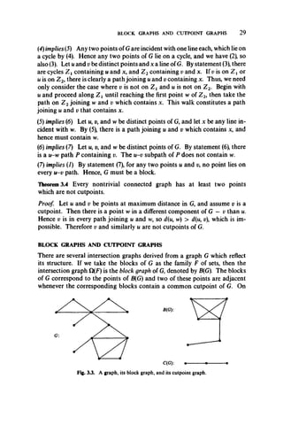
![36 TREES
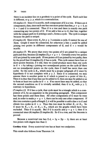
Fig. 4.3. The weights at the points of a tree.
nonendpoints of the tree in Fig. 4.3 are indicated. Of course the weight at
each endpoint is 14, the number of lines.
A point v is a centroid point of a tree T if v has minimum weight, and the
centroid of T consists of all such points. Jordan [J2] also proved a theorem
on the centroid of a tree analogous to his result for centers.
Theorem 4.3 Every tree has a centroid consisting of either one point or two
adjacent points.
The smallest trees with one and two central and centroid points are
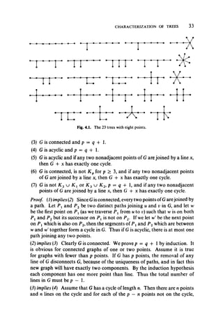
shown in Fig. 4.4.
1
Centroid
2
Fig. 4.4. Trees with all combinations of one or two central and centroid points.
BLOCK-CUTPOINT TREES
It has often been observed that a connected graph with many cutpoints
bears a resemblance to a tree. This idea can be made more definite by as
sociating with every connected graph a tree which displays the resemblance.
For a connected graph G with blocks {£,} and cutpoints {<;,}, the
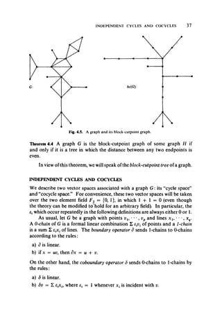
block-cutpoint graph of G, denoted by bc(G), is defined as the graph having
point set {£J u {cj}, with two points adjacent if one corresponds to a block
Bi and the other to a cutpoint Cj and Cj is in £ f. Thus bc(G) is a bigraph. This
concept was introduced in Harary and Prins [HP22] and also in Gallai
[G3]. (See Fig. 4.5.)
1 Center 2
•
— <
— <](https://image.slidesharecdn.com/graphtheory-181103155731/85/Graph-theory-47-320.jpg)
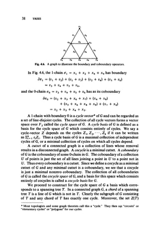
![4 0 TREES
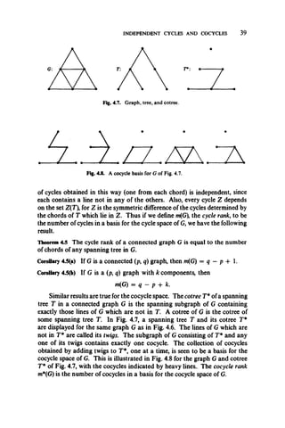
Theorem 4.6 The cocycle rank of a connected graph G is the number of
twigs in any spanning tree of T.
As in the case of cycles, we have two immediate corollaries.
Corollary 4.6(a) If G is a connected (p, q) graph, then m*(G) = p — 1.
Corollary 4.6(b) If G is a (p, q) graph with k components, then m*(G) = p — k.
Excursion
The 1-dimensional case of an important general result about simplicial
complexes can be derived from Theorem 4.5. The Euler-Poincare equation
a0 - a, + a2 - • • • = p0 - + p2 - • • •,
where the /?„ are the Betti numbers and the a„ are the numbers of simplexes
of each dimension, holds for every simplicial complex. Recall from Chapter 1
that every graph is a simplicial complex, with its points 0-simplexes and its
lines 1-simplexes. Foragraph,/?0 = fc, the number ofconnected components,
and fii = m(G), the number of independent cycles of G. Since no graph
contains an n-simplex with n > 1, a„ = /?„ = 0, for all n > 1. Thus
ao ~ a i = Po — Pi so p — q = k — m(G) and we see that Corollary 4.5(b)
is the Euler-Poincare equation for graphs.
MATROIDS
This subject was first introduced by Whitney [W15]. A discussion of the
basic properties of matroids, as well as several equivalent axiomatic formula
tions, may be found in Whitney’s original paper.
A matroid consists of a finite set M of elements together with a family
= { c1# C2, • • •} of nonempty subsets of M, called circuits, satisfying the
axioms:
1. no proper subset of a circuit is a circuit;
2. if x e C 1 n C2, then C x u C2 — {x} contains a circuit.
With every graph G, one can associate a matroid by taking its set X of
lines as the set Af, and its cycles as the circuits. It is easily seen that the two
axioms are satisfied. It is slightly less obvious that G yields another matroid
by taking the cocycles of G as the circuits. These are called respectively the
cycle matroid and the cocycle matroid of G.
Another, equivalent, definition of matroid is as follows. Amatroid
consists of a finite set M of elements together with a familyof subsets of M
called independent sets such th at:
1. the empty set is independent;](https://image.slidesharecdn.com/graphtheory-181103155731/85/Graph-theory-51-320.jpg)
![MATROIDS 41
2. every subset of an independent set is independent;
3. for every subset A of M, all maximal independent sets contained in A
have the same number of elements.
A graph G yields a matroid in this sense by taking the lines of G as set
M and the acyclic subgraphs of G as the independent sets.
The duality (cycles vs. cocycles, trees vs. cotrees) which appears in the
preceding section is closely related to duality in matroids. Minty [M l2]
constructed a self-dual axiom system for “graphoids” which displays matroid
duality explicitly.
A graphoid consists of a set M of elements together with two collections
^ and Q) of nonempty subsets of M, called circuits and cocircuits respectively,
such th at:
1. for any C e ^ and D e |C n D| ^ 1;
2. no circuit properly contains another circuit and no cocircuit properly
contains another cocircuit;
3. for any painting of M which colors exactly one element green and the
rest either red or blue, there exists either
a) a circuit C containing the green element and no red elements, or
b) a cocircuit D containing the green element and no blue elements.
While the cycles of every graph form a matroid, not every matroid can
so arise from a graph, as we shall see in Chapter 13. Two comprehensive
references on matroid theory are Minty [M12] and Tutte [T19].
Excursion
Ulam’s conjecture is still as unsolved as ever for arbitrary graphs. But
Kelly [K5] proved its validity for trees. As we have seen, the point of view
toward this conjecture proposed in [H29] is that if G has p > 3 and one is
presented with the p unlabeled subgraphs G, = G — vi9 then the graph G
itself can be reconstructed uniquely from the Gt. Kelly’s result for trees
was extended in [HP6] where it is shown that every nontrivial tree T can be
reconstructed from only those subgraphs T{ = T — v{which are themselves
trees, that is, such that v(is an endpoint. This has been improved, in turn, by
Bondy, who showed [B15] that a tree T can be reconstructed from its
subgraphs T — with the the peripheral points, those whose eccentricity
equals the diameter of T. Manvel [M2] then showed that almost* every tree
T can be reconstructed using only those subtrees T — which are non
isomorphic. Another class of graphs has been reconstructed by Manvel
[M3], namely unicyclic graphs, which are connected and have just one cycle.
* With just two pairs of exceptional trees.](https://image.slidesharecdn.com/graphtheory-181103155731/85/Graph-theory-52-320.jpg)
![4 2 TREES
EXERCISES
4.1 Draw all trees with nine points. Then compare your diagrams with those in
Appendix II.
4.2 Every tree is a bigraph. Which trees are complete bigraphs?
4.3 The following four statements are equivalent.
(1) G is a forest.
(2) Every line of G is a bridge.
(3) Every block of G is X 2.
(4) Every nonempty intersection of two connected subgraphs of G is connected.
4.4 The following four statements are equivalent.
(1) G is unicyclic.
(2) G is connected and p = q.
(3) For some line x of G, the graph G - x is a tree.
(4) G is connected and the set of linesof G which are not bridges form a cycle.
4.5 For any connected graph G, r(G) < d(G) < 2r(G).
4.6 Construct a tree with disjoint center and centroid, each having two points.
4.7 The center of any connected graph lies in a block. (Harary and Norman [HN2])
4.8 Given the block-cutpoint tree bc(G) of a connected graph G, determine the block-
graph B(G) and the cutpoint-graph C(G).
4.9 Determine the cycle ranks of (a) Kpi (b) Km (c) a connected cubic graph with
p points.
4.10 The intersection of a cycle and a cocycle contains an even number of lines.
4.11 A graph is bipartite if and only if every cycle in some cycle basis is even.
4.12 Every connected graph has a spanning tree.
4.13 Show how the block-cutpoint graph ofany graph can be defined as an intersection
graph.
4.14 A cotree of aconnected graph is a maximal subgraph containing no cocycles.
4.15 A tree with p> 3 has diameter 2 if and only if it is astar.
4.16 Prove or disprove:
a) If G has diameter 2, then it has a spanning star.
b) If G has a spanning star, then it has diameter 2.
4.17 Determine all connected graphs G for which G = bc(G).
*418 The maximum number of lines in a graph with p points and radius r is
(Anderson and Harary [AH1])
[pip ~ 2)/2] if r = 2,
4(p2 ~ 4rp H- 5p -f- 4r2 - 6r) if r > 3. (Vizing [V5])
4.19 G is a block if and only if every two lines lie on a common cocycle.](https://image.slidesharecdn.com/graphtheory-181103155731/85/Graph-theory-53-320.jpg)
![C H A P T E R 5
CONNECTIVITY
We must all hang together,
or assuredly we shall all hang separately.
B. F r a n k l in
The connectivity of graphs is a particularly intuitive area of graph theory
and extends the concepts of cutpoint, bridge, and block. Two invariants
called connectivity and line-connectivity are useful in deciding which of two
graphs is “more connected.”
There is a rich body of theorems concerning connectivity. Many of
these are variations of a classical result of Menger, which involves the number
of disjoint paths joining a given pair of points in a graph. We will see that
several such variations have been discovered in areas of mathematics other
than graph theory.
CONNECTIVITY AND LINE-CONNECTIVITY
The connectivity k = k(G) of a graph G is the minimum number of points
whose removal results in a disconnected or trivial graph. Thus the con
nectivity of a disconnected graph is 0, while the connectivity of a connected
graph with a cutpoint is 1. The complete graph K pcannot be disconnected
by removing any number of points, but the trivial graph results after re
moving p - 1 points; therefore, k(Kp) = p - 1. Sometimes k is called the
point-connectivity.
Analogously, the line-connectivity X = X(G) of a graph G is the minimum
number of lines whose removal results in a disconnected or trivial graph.
Thus X(Kt) = 0 and the line-connectivity of a disconnected graph is 0, while
that of a connected graph with a bridge is 1. Connectivity, line-connectivity,
and minimum degree are related by an inequality due to Whitney [W ll].
Theorem 5.1 For any graph G,
k(G) < X(G) < <5(G).
43](https://image.slidesharecdn.com/graphtheory-181103155731/85/Graph-theory-54-320.jpg)
![4 4 CONNECTIVITY
Proof. We first verify the second inequality. If G has no lines, then X = 0.
Otherwise, a disconnected graph results when all the lines incident with a
point of minimum degree are removed. In either case, X < <5.
To obtain the first inequality, various cases are considered. If G is
disconnected or trivial, then k = X = 0. If G is connected and has a bridge x,
then X = . In this case, k = 1 since either G has a cutpoint incident with x
or G is K 2. Finally, suppose G has X > 2 lines whose removal disconnects
it. Clearly, the removal of X — 1 of these lines produces a graph with a
bridge x = uv. For each ofthese X — 1lines, select an incident point different
from u or v. The removal of these points also removes the X — 1 lines and
quite possibly more. If the resulting graph is disconnected, then k < X; if
not, x is a bridge, and hence the removal of u or v will result in either a
disconnected or a trivial graph, so k < X in every case. (See Fig. 5.1.)
Chartrand and Harary [CH4] constructed a family of graphs with
prescribed connectivities which also have a given minimum degree. This
result shows that the restrictions on tc, X, and <5 imposed by Theorem 5.1
cannot be improved.
Theorem 5.2 For all integers a, b, c such that 0 < a < b < c, there exists a
graph G with k(G) = a, X(G) = b, and (5(G) = c.
Chartrand [C8] pointed out that if S is large enough, then the second
inequality of Theorem 5.1 becomes an equality.
Theorem 5.3 If G has p points and (5(G) > [p/2], then A(G) = (5(G).
For example, if G is regular of degree r > p/2, then A(G) = r. In
particular, X(Kp) = p — 1.
The analogue of Theorem 5.3 for connectivity does not hold. The
problem of determining the largest connectivity possible for a graph with a
given number ofpoints and lines was proposed by Berge [B11] and a solution
was given in [H26].
Theorem 5.4 Among all graphs with p points and q lines, the maximum
connectivity is 0 when q < p — 1 and is [2g/p], when q > p — 1.](https://image.slidesharecdn.com/graphtheory-181103155731/85/Graph-theory-55-320.jpg)
![CONNECTIVITY AND LINE-CONNECTIVITY 4 5
Outline ofproof Since the sum of the degrees of any (p, q) graph G is 2q, the
mean degree is 2q/p. Therefore <5(G) < [2q/p], so k(G) < 2q/p] by Theorem
5.1. To show that this value can actually be attained, an appropriate family
of graphs can be constructed. The same construction also gives those
(p, q) graphs with maximum line-connectivity.
Corollary 5.4(a) The maximum line-connectivity of a (p, q) graph equals the
maximum connectivity.
Only very recently the question of separating a graph by removing a
mixed set of points and lines has been studied. A connectivity pair of a graph
G is an ordered pair (a, b) of nonnegative integers such that there is some set
of a points and b lines whose removal disconnects the graph and there
is no set of a — 1 points and b lines or of a points and b — 1 lines with this
property. Thus in particular the two ordered pairs (k, 0) and (0, X) are
connectivity pairs for G, so that the concept of connectivity pair generalizes
both the point-connectivity and the line-connectivity of a graph. It is readily
seen that for each value of a, 0 < a < k , there is a unique connectivity pair
(a, ba); thus G has exactly k + 1 connectivity pairs.
The connectivity pairs of a graph G determine a function / from the
set (0, 1, • • •, k:} into the nonnegative integers such that /(k) = 0 (cf.
Theorem 5.1). This is called the connectivity function of G. It is strictly
decreasing, since if (a, b) is a connectivity pair with b > 0 there is obviously
a set of a + 1 points and b — 1 lines whose removal disconnects the graph
or leaves only one point. The following theorem, proved by construction in
Beineke and Harary [BH6], shows that these are the only conditions which
a connectivity function must satisfy.
Theorem 5.5 Every decreasing function / from {0, 1, •• •, k } into the non
negative integers such that /(k) = 0 is the connectivity function of some
graph.
A graph G is n-connected if *c(G) > n and n-line-connected if 2(G) > n.
We note that a nontrivial graph is 1-connected if and only if it is connected,
and that it is 2-connected if and only if it is a block having more than one
line. So K 2 is the only block not 2-connected. From Theorem 3.3, it
therefore follows that G is 2-connected if and only if every two points of G
lie on a cycle. Dirac [D8] extended this observation to n-connected
graphs.
Theorem 5.6 If G is n-connected, n > 2, then every set of n points of G lie
on a cycle.
By taking G to be the cycle Cn itself, it is seen that the converse is not
true for n > 2.
A characterization of 3-connected graphs also exists, although its
formulation is not as easily given. In order to present this result, we need](https://image.slidesharecdn.com/graphtheory-181103155731/85/Graph-theory-56-320.jpg)
![4 6 CONNECTIVITY
the “wheel” invented by the eminent graph theorist W. T. Tutte. For n > 4,
the wheel Wn is defined to be the graph K x + C„_,. (See Fig. 5.2.)
Tutte’s theorem [T13] characterizing 3-connected graphs can now be
stated.
Theorem 5.7 A graph G is 3-connected if and only if G is a wheel or can be
obtained from a wheel by a sequence of operations of the following two
types:
1. The addition of a new line.
2. The replacement of a point v having degree at least 4 by two adjacent
points v', v" such that each point formerly joined to v is joined to exactly
one of vfand v”so that in the resulting graph, deg v' > 3 and deg v" > 3.
The graph G of Fig. 5.3 is 3-connected since it can be obtained from the
wheel W5 as indicated.
An n-component of a graph G is a maximal n-connected subgraph. In
particular, the 1-components of G are the nontrivial components of G while
the 2-components are the blocks of G with at least 3 points. It is readily
seen that two different 1-components have no points in common, and two
Fig. 5.3. Demonstration that a graph is 3-connected.](https://image.slidesharecdn.com/graphtheory-181103155731/85/Graph-theory-57-320.jpg)
![GRAPHICAL VARIATIONS OF MENGER’S THEOREM 4 7
Fig. 5.4. A graph with two 3-components which meet in two points.
distinct 2-components meet in at most one point. These facts have been
generalized by Harary and Kodama [HK1]. (See Fig. 5.4.)
Theorem 5.8 Two distinct n-components of a graph G have at most n — 1
points in common.
GRAPHICAL VARIATIONS OF MENGER’S THEOREM
In 1927 Menger [M9] showed that the connectivity of a graph is related to
the number of disjoint paths joining distinct points in the graph. Many
of the variations and extensions of Monger’s result which have since appeared
have been graphical, and we discuss some of these here. By emphasizing the
form these theorems take, it is possible to classify them in an illuminating
way.
Let u and v be two distinct points of a connected graph G. Two paths
joining u and v are called disjoint (sometimes called point-disjoint) if they
have no points other than u and v (and hence no lines) in common; they are
line-disjoint ifthey have no lines in common. A set S of points, lines, or points
and lines separates u and v if u and v are in different components of G —5.
Clearly, no set of points separates two adjacent points. Menger’s Theorem
was originally presented in the “point form” given in Theorem 5.9.
Theorem 5.9 The minimum number of points separating two nonadjacent
points s and t is the maximum number of disjoint s-t paths.
Proof. We follow the elegant proof of Dirac [DIO]. It is clear that if k
points separate s and t, then there can be no more than k disjoint paths
joining s and t.
It remains to show that if it takes k points to separate s and t in G, there
are k disjoint s-t paths in G. This is certainly true if k = 1. Assume it is not
true for some k > 1. Let h be the smallest such k, and let F be a graph with
the minimum number of points for which the theorem fails for h. We
remove lines from F until we obtain a graph G such that h points are required
to separate s and t in G but for any line x of G, only h — 1points are required to
separate s and tin G - x. We first investigate the properties of this graph G,
and then complete the proof of the theorem.](https://image.slidesharecdn.com/graphtheory-181103155731/85/Graph-theory-58-320.jpg)
![4 8 CONNECTIVITY
By the definition of G, for any line x of G there exists a set S(x) of h — 1
points which separates s and t in G —x. Now G — S(x) contains at least
one s-t path, since it takes h points to separate s and t in G. Each such s-t
path must contain the line x = uv since it is not a path in G — x. So
m, v $ S(x) and if u ^ s, t then S(x) u {u} separates s and t in G.
If there is a point w adjacent to both s and t in G, then G — w requires
h — 1 points to separate s and t and so it has h — 1 disjoint s-t paths.
Replacing w, we have h disjoint s-t paths in G. So we have shown:
(I) No point is adjacent to both s and t in G.
Let W be any collection of h points separating s and t in G. An s-W
path is a path joining s with some e W and containing no other point of
W. Call the collections ofall s-W paths and W -t paths Psand Pt respectively.
Then each s-t path begins with a member of Ps and ends with a member of
Pt, because every such path contains a point of W. Moreover, the paths in
Ps and Pt have the points of W and no others in common, since it is clear
that each w, is in at least one path in each collection and, if some other point
were in both an s-W and a W -t path, then there would be an s-t path con
taining no point of W. Finally, either Ps — W = {s} or Pt — W = {t},
since, if not, then both Ps plus the lines {wjt, w2t, • *•} and Pt plus the lines
{swl5 sw2, • * } are graphs with fewer points than G in which s and t are
nonadjacent and /j-connected, and therefore in each there are h disjoint
s-t paths. Combining the s-W and W -t portions of these paths, we can
construct h disjoint s-t paths in G, and thus have a contradiction. Therefore
we have proved:
(II) Any collection W of h points separating s and t is adjacent either to
s or to t.
Now we can complete the proofofthe theorem. Let P = {s, uu m2, •*•, t}
be a shortest s-t path in G and let ulu2 = x. Note that by (I), u2 ^ t. Form
S(x) = {vt, v2, " ,v h^ 1} as above, separating s and t in G —x. By (I),
uxt i G, so by (II), with W = S(x) u {i^}, sv( e G, for all i. Thus by (I),
vtt 4 G, for all i. However, if we pick W = S(x) u {u2} instead, we have by
(II) that su2 e G, contradicting our choice of P as a shortest s-t path, and
completing the proof of the theorem.
In Fig. 5.5 we display a graph with two nonadjacent points s and t
which can be separated by removing three points but no fewer. In accordance
with the theorem, the maximum number of disjoint s-t paths is 3.
Chronologically the second variation of Menger’s Theorem was pub
lished by Whitney in a paper [W ll] in which he included a criterion for a
graph to be n-connected.
Theorem 5.10 A graph is w-connected if and only if every pair of points are
joined by at least n point-disjoint paths.](https://image.slidesharecdn.com/graphtheory-181103155731/85/Graph-theory-59-320.jpg)
![GRAPHICAL VARIATIONS OF MENGER’S THEOREM 4 9
Fig. 5.5. A graph illustrating Menger s Theorem.
An indication of the relationship between Theorems 5.9 and 5.10 is easily
supplied by introducing the concept of local connectivity. The local con
nectivity of two nonadjacent points u and v of a graph is denoted by k ( u , v)
and is defined as the smallest number of points whose removal separates
u and v. In these terms, Menger’s Theorem asserts that for any two specific
nonadjacent points u and p, k(w, v) = /z0(w, v), the maximum number of
point-disjoint paths joining u and p. Obviously both theorems hold for
complete graphs. If we are dealing with a graph G which is not complete,
then the observation which links Theorems 5.9 and 5.10 is that k(G) =
min k(u, v) over all pairs of nonadjacent points u and v.
Strangely enough, the theorem analogous to Theorem 5.9 in which the
pair of points are separated by a set of lines was not discovered until much
later. There are several nearly simultaneous discoveries of this result whichr
appeared in papers by Ford and Fulkerson [FF1] (as a special case of their
“max-flow, min-cut” theorem) and Elias, Feinstein, and Shannon [EFS1],
and also in unpublished work of A. Kotzig.
Theorem 5.11 For any two points of a graph, the maximum number of line-
disjoint paths joining them equals the minimum number of lines which
separate them.
Referring again to Fig. 5.5, we see that s and t can be separated by
the removal of five lines but no fewer, and that the maximum number of
line-disjoint s-t paths is five.
Even with only these three theorems available, we can see the beginnings
of a scheme for classifying them. The difference between Theorems 5.9 and
5.10 may be expressed by saying that Theorem 5.9 involves two specific
points of a graph while Theorem 5.10 gives a bound in terms of two general
points. This distinction, as well as the obvious one between Theorems 5.9
and 5.11, is indicated in Table 5.1.
Thus we see that with no additional effort we can get another variation of
Menger’s Theorem by stating the line form of the Whitney result.](https://image.slidesharecdn.com/graphtheory-181103155731/85/Graph-theory-60-320.jpg)
![50 CONNECTIVITY
Table 5.1
Theorem Objects separated Maximum number Minimum number
5.9 specific m, v disjoint paths points separating w, v
5.10 general w, v disjoint paths points separating u, v
5.11 specific uf v line-disjoint paths lines separating u, v
Theorem 5.12 A graph is n-line-connected if and only if every pair of points
are joined by at least n line-disjoint paths.
In Menger’s original paper there also appeared the following variation
involving sets of points rather than individual points.
Theorem 5.13 For any two disjoint nonempty sets of points Vx and the
maximum number ofdisjoint paths joining Vxand V2is equal to the minimum
number of points which separate Vx and V2.
Of course it must be specified that no point of Vx is adjacent with a
point of V2 for the same reason as in Theorem 5.9. Two paths joining Vx
and V2 are understood to be disjoint if they have no points in common other
than their endpoints. A proof of the equivalence of Theorems 5.9 and 5.13
is extremely straightforward and only involves shrinking the sets of points
Vx and V2 to individual points.
Another variation is given in the next theorem, considered by Dirac
[D9]. Because the proof involves typical methods in the demonstration of
equivalence of these variations, we include it in full.
Theorem 5.14 A graph with at least 2n points is n-connected if and only if
for any two disjoint sets Vx and V2 of n points each, there exist n disjoint
paths joining these two sets of points.
Note that in this theorem these n disjoint paths do not have any points
at all in common, not even their endpoints!
Proof, To show the sufficiency of the condition, we form the graph G' from
G by adding two new points wx and w2 with vvfadjacent to exactly the points
of Vi9 i = 1, 2. (See Fig. 5.6.)
Since G is n-connected, so is G', and hence by Theorem 5.9 there are n
disjoint paths joining wt and w2. The restrictions of these paths to G are
clearly the n disjoint Vx-V2 paths we need.
To prove the other “half,” let S be a set of at least n — 1 points which
separates G into Gx and G2, with points sets V and V2 respectively. Then,
since V > 1, V'2 > 1, and V + V2 + S = V > 2n, there is a
partition of S into two disjoint subsets S x and S2 such that V u S x > n
and |V2 u S2| ^ ft. Picking any n-subsets Vx of Vj u S X9and V2 of V’2 u S2,](https://image.slidesharecdn.com/graphtheory-181103155731/85/Graph-theory-61-320.jpg)
![GRAPHICAL VARIATIONS OF MENGER’S THEOREM 51
Fig. 5.6. Construction of G
we have two disjoint sets of n points each. Every path joining Vt and V2
must contain a point of S, and since we know there are n disjoint Vx-V 2
paths, we see that |S| > n, and G is n-connected.
We have defined connectivity pairs for a graph. Similarly, one can define
connectivity pairs for two specific points u and v. It is then natural to ask for
a mixed form of Menger’s Theorem involving connectivity pairs. The
following theorem of Beineke and Harary [BH6] is one such result; a proof
can be readily supplied by imitating that of Theorem 5.9.
Theorem 5.15 The ordered pair (a, b) is a connectivity pair for points u and v
in a graph G if and only if there exist a point-disjoint u-v paths and also b
line-disjoint u-v paths which are line-disjoint from the preceding a paths,
and further these are the maximum possible numbers of such paths.
In general, all of the theorems we have mentioned have corresponding
digraph forms, and in fact Dirac points out that his proof of Menger’s
Theorem works equally well for directed graphs. At this point, then, we
could add eleven more theorems to Table 5.1, namely Theorems 5.12 through
5.15, and the directed forms of Theorems 5.9 through 5.15. This would be a
somewhat futile effort, however, since it should be clear that the table would
still be far from complete. To count the total number of variations which
have been suggested up to this point, we note that we may consider either a
graph G or a digraph Z), in which we may separate
i) specific points u, v,
ii) general points w, v,
iii) two sets of points Vl9 V2 (as in Theorem 5.13).
This separation may be accomplished by removing
i) points,
ii) lines, or
iii) points and lines (as in Theorem 5.15).](https://image.slidesharecdn.com/graphtheory-181103155731/85/Graph-theory-62-320.jpg)
![52 CONNECTIVITY
By taking all possible combinations of these alternatives, we could
construct 2 - 3 - 3 = 18 theorems. The fact that all of these theorems are
true may be verified by the reader, although it would be a tedious exercise.
Finally, Fulkerson [F13] proved the following theorem, which deals
with disjoint cutsets instead of disjoint paths.
Theorem 5.16 In any graph, the maximum number of line-disjoint cutsets
of lines separating two points u and v is equal to the minimum number of
lines in a path joining u and v ; that is, to d(u9v).
Although this theorem is of Mengerian type, it is much easier to prove
than M^fTger’s Theorem. By taking all the possible variations of this theorem,
as we have with the theorems involving paths, we could increase the number
of Mengerian theorems again.
FURTHER VARIATIONS OF MENGER’S THEOREM
In this section we include several additional variations of Menger’s Theorem,
all discovered independently and only later seen to be related to each other
and to a graph theoretic formulation.
A network N may be regarded as a graph or directed graph together with
a function which assigns a positive real number to each line. For precise
definitions of “maximum flow” and “minimum cut capacity,” see the book
[FF2] by Ford and Fulkerson.
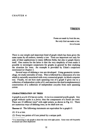
Fig. 5.7. A network with integral capacities.
Theorem 5.17 In any network N in which there is a path from u to v, the
maximum flow from u to v is equal to the minimum cut capacity.
It is straightforward but not entirely obvious to verify that in Fig. 5.7
the maximum flow in the network from u to v is 7, and that the minimum
cut capacity is also 7.
In the case where all the capacities are positive integers, as in this net
work, there is an immediate equivalence between the maximum flow theorem
and that variation of Menger’s Theorem in which the setting is a directed
multigraph D and there are two specific points u and v. The transformation](https://image.slidesharecdn.com/graphtheory-181103155731/85/Graph-theory-63-320.jpg)
![FURTHER VARIATIONS OF MENGER’S THEOREM 53
Fig. 5.8. The transformation from network to multigraph.
which makes this equivalence apparent is displayed in Fig. 5.8 in which
the directed line from u to vx in Fig. 5.7 which has capacity 3 is transformed
into three directed lines without any capacity indicated.
Let us define a line of a matrix as either a row or a column. In a binary
matrix M, a collection of lines is said to cover all the unit entries of M
if every 1 is in one of these lines. Two l’s of M are called independent if they
are neither in the same row nor in the same column. Konig [K9] obtained
the next variation of Menger’s Theorem in these term s; compare Theorem
10.2.
Theorem 5.18 In any binary matrix, the maximum number of independent
unit elements equals the minimum number of lines which cover all the units.
'0 0 1 0 0 o" 0 0 1 0 0 o'
1 1 0 1 0 1 1 0 0 0 0 0
0 0 1 0 0 1 M' = 0 0 0 0 0 1
0 1 1 0 1 0 0 1 0 0 0 0
0 0 1 0 0 1 0 0 0 0 0 0
We illustrate Theorem 5.18 with the binary matrix M above. All the
unit entries of M are covered by rows 2 and 4 and columns 3 and 6, but there
is no collection of three lines of M which covers all its l’s. In the matrix M'
there are shown four independent unit entries of M and there is no set of five
independent l’s in M.
When this matrix M is regarded as an incidence matrix of sets versus
elements, Theorem 5.18 becomes very closely related to the celebrated
theorem of P. Hall [H8], which provides a criterion for a collection of finite
sets Sl9 S2, **•, Sm to possess a system of distinct representatives. This
means a set {el9 e2i - *, em} of distinct elements such that etis in S„ for each i.
We present here the proof of Hall’s Theorem which is due to Rado [R l].
Theorem 5.19 There exists a system of distinct representatives for a family
of sets S i9 S2, ' , S mif and only if the union of any k of these sets contains
at least k elements, for all k from 1 to m.
Proof The necessity is immediate. For the sufficiency we first prove that if
the collection {5f}satisfies the stated conditions and |SJ > 2, then there is an
element e in Smsuch that the collection of sets S u S2, • • *, Sm-i, Sm — {e}](https://image.slidesharecdn.com/graphtheory-181103155731/85/Graph-theory-64-320.jpg)
![54 CONNECTIVITY
also satisfies the conditions. Suppose this is not the case. Then there are
elements e and /in Smand subsets J and K of {1, 2, • • •, m — 1} such that
which is a contradiction.
The sufficiency now follows by induction on the maximum of the
numbers |Sf|. If each set is a singleton, there is nothing to prove. The in
duction step is made by application (repeated if necessary) of the above
result to the sets of largest order.
In Fig. 5.9 we show a bipartite graph B in which the points refer either to
sets Si or to elements Two points of B are adjacent if and only if one is a
set point, the other is an element point, and the element is a member of the
set. The link between Theorem 5.19 and Menger’s Theorem is accomplished
by introducing two new points into a graph of the form of Fig. 5.9. Call
these points u and v and join u to every set point St and v with every element
point dj to obtain a new graph. Theorem 5.19 can then be proved by applying
either the maximum flow theorem or the appropriate line form of Menger’s
Theorem to this graph.
Although the following theorem due to Dilworth [D4] is expressed in
terms of lattice theory,* it has been established (see Mirsky and Perfect
[MP1]) that the result is equivalent to Hall’s Theorem. Two elements of a
lattice (see Birkhoff [B13]) are incomparable if neither dominates the other.
and
But then
|/| + K > |(u s.) U (Sm - {e}) + |(u s,) u (Sm - {/})
> J u K | + 1 + J n K > |J| + |/q,
B:
Fig. 5.9. A bipartite graph illustrating Hall’s Theorem.
* More generally the result holds for partially ordered sets.](https://image.slidesharecdn.com/graphtheory-181103155731/85/Graph-theory-65-320.jpg)
![EXERCISES 55
By a chain in a lattice is meant a downward path from an upper element to a
lower element in the “Hasse diagram” of the lattice.
Theorem 5.20 In any finite lattice, the maximum number of incomparable
elements equals the minimum number of chains which include all the
elements.
For example, in the lattice of the 3-cube, there are at most three incom
parable elements; it is easy to cover all the elements with three chains but
impossible to do so with only two chains.
We have seen in this section several theorems of Mengerian type
occurring in settings which are not graph theoretic. A more extensive
treatment of such results appears in the review article [H33]. For an elegant
summary of the vast literature on theorems involving systems of distinct
representatives, see Mirsky and Perfect [MP1].
EXERCISES
5.1 The connectivity of
a) the octahedron K2 + C4 is 4.
b) the square of a polygon C„, n > 5, is 4.
5.2 Every n-connected graph has at least pn/2 lines.
5.3 Construct a graph with k = 3, X — 4, <5 = 5.
5.4 Theorem 5.3 does not hold if X(G) is replaced by ic(G).
5.5 There exists no 3-connected graph with seven lines.
5.6 The connectivity and line-connectivity are equal in every cubic graph.
5.7 Determine which connectivity pairs can occur in 4-regular graphs.
5.8 If G is regular of degree r and k — 1, then X < [r/2].
5.9 Construct a family of (p, q) graphs with 2q/p integral such that k —2q/p.
5.10 Let G be a complete n-partite graph other than C4. Then every minimum line
cutset is the coboundary of some point. (M. D. Plummer)
5.11 Find the connectivity function for s and t in the graph of Fig. 5.5.
5.12 Find a graph with points s and t for which the connectivity function is (0, 5), (1, 3),
(2, 2 (3, 0).
5.13 Use Tutte’s Theorem 5.7 to show that the graph of the cube Q3is 3-connected.
5.14 Every block of a connected graph G is a wheel if and only if q = 2p - 2 and
k(u, v) = 1 or 3 for any two nonadjacent points u, v. (Bollobas [B14])
5.15 Every cubic triply-connected graph can be obtained from KA by the following
construction. Replace two distinct lines and u2v2 (u { = u 2 is permitted) by the
subgraph with two new points w l9 w2 and the new lines iqwj, WjWj, u 2w 2, w 2v2y and
WlW2.](https://image.slidesharecdn.com/graphtheory-181103155731/85/Graph-theory-66-320.jpg)
![56 CONNECTIVITY
5.16 Given two disjoint paths Px and P2joining two points u and v of a 3-connected
graph G, is it always possible to find a third path joining u and v which is disjoint from
both Pxand P2?
5.17 State the result analogous to Theorem 5.9 for the maximum number of disjoint
paths joining two adjacent points of a graph.
*5.18 Iffr(p) is the smallest number such that for q > fr(p) every (p, q) graph has two
points joined by r disjoint paths, then
flip) = A M p) = [<3p - m l and Up) = 2p - 1.
(Bollobas [B14])
5.19 If G has diameter d and k > 1, then p > tc(d — 1) + 2. (Watkins [W5])
5.21 If G is connected, then
k(G) =1-1- min tc(G —u)
veV
5.22 In any graph, the maximum number of disjoint cutsets of points separating two
points u and v equals d(u, v) — 1.
5.23 In a K-minimal graph G, k(G — x) < k(G ) for every line x.
a) Gis ic-minimal ifand only if k(u, u) = k(G ) for every pair of adjacent points u, v.
b) If G is jc-minimal then S = k. (Halin [H5]) ’
5.24 Prove the equivalence of Theorems 5.18 and 5.19. (See for example M. Hall
[H7, p. 49]).
5.25 If G is n-connected, n > 2, and <S(G) > (3n — l)/2, then there exists a point v in G
such that G — v is n-connected. (Chartrand, Kaugars, and Lick [CKL1])](https://image.slidesharecdn.com/graphtheory-181103155731/85/Graph-theory-67-320.jpg)
![58 PARTITIONS
di < p — 1, and n is even. These two conditions are not sufficient for a
partition to be graphical, as shown by the partition 10 = 3 + 3 + 3 + 1.
Two related questions arise. First, how can one tell whether a given partition
is graphical? Second, how can one construct a graph for a given graphical
partition? An existential answer to the first was given by Erdos and Gallai
[EG1]. Another answer found independently by Havel [H36] and Hakimi
[H4] is constructive in nature, and so answers the second question as well.
We first give this result.
Theorem 6.1 A partition II = (du d2, " , dp) of an even number into p
parts with p — 1 > dx > d2 > **• > dp is graphical if and only if the
modified partition
IT = (d2 — 1, d2 — 1, • • •, ddi + j — 1, ddl +2, • • •, dp)
is graphical.
Proof. If IT is graphical, then so is n , since from a graph with partition II'
one can construct a graph with partition II by adding a new point adjacent
to points of degrees d2 — 1, d3 — I, • • •9ddl +i — 1.
Now let G be a graph with partition II. If a point of degree dxis adjacent
to points of degrees d( for i = 2 to dx + 1, then the removal of this point
results in a graph with partition II'.
Therefore we will show that from G one can get a graph with such a
point. Suppose that G has no such point. We assume that in G, point v4has
degree dh with vx being a point of degree dx for which the sum of the degrees
of the adjacent points is maximum. Then there are points v{ and Vj with
d( > dj such that vxVj is a line but vxv( is not. Therefore some point vk is
adjacent to vt but not to Vj. Removal of the lines vxVj and vkvt and addition
of vxVi and ykVj results in another graph with partition II in which the sum
of the degrees of the points adjacent to vx is greater than before. Repeating
this process results in a graph in which vx has the desired property.
The theorem gives an effective algorithm for constructing a graph with a
given partition, if one exists. If none exists, the algorithm cannot be applied
at some step.
Corollary 6.1 (Algorithm) A given partition II = (dx, d2, • • •, dp) with
p - 1 > dx > d2 > • • • > dp
is graphical if and only if the following procedure results in a partition with
every summand zero.
1. Determine the modified partition II' as in the statement of Theorem 6.1.
2. Reorder the terms of II' so that they are nonincreasing, and call the
resulting partition IIx.](https://image.slidesharecdn.com/graphtheory-181103155731/85/Graph-theory-69-320.jpg)
![PARTITIONS 59
Fig. 6.2. An example of the algorithm for graphical partitions.
3. Determine the modified partition FI" of U l as in step 1, and the re
ordered partition U 2.
4. Continue the process as long as nonnegative summands can be obtained.
If a partition obtained at an intermediate stage is known to be graphical,
stop, since Ef itselfis then established as graphical. To illustrate this algorithm,
we test the partition
n= (5, 5, 3, 3, 2, 2, 2)
IT = ( 4,2,2, 1,1,2)
III = ( 4, 2, 2, 2, 1, 1)
i r = ( 1, 1, i, o, i).
Clearly II" is graphical, so II is also graphical. The graph so constructed is
shown in Fig. 6.2.
The theorem of Erdos and Gallai [EG1] is existential in nature, but its
proof uses the same construction.
Theorem 6.2 Let n = (dlJ d2, • • • , dp) be a partition of 2q into p > 1 parts,
dt > d 2 > - > d p. Then n is graphical if and only if for each integer r,
1 < r < p — 1,
X X < r(r - 1) + X m«n {»•>4}. (6.1)
i=l i=r+1
Proof. The necessity of these conditions (6.1) is straightforward. Given
that n is a partition of 2q belonging to a graph G, the sum of the r largest
degrees can be considered in two parts, the first being the contribution to this
sum of lines joining the corresponding r points with each other, and the
second obtained from lines joining one of these r points with one of the
remaining p — r points. These two parts are respectively at most r(r - l)and
S?=r+1 min {r, <*,}.](https://image.slidesharecdn.com/graphtheory-181103155731/85/Graph-theory-70-320.jpg)
![62 PARTITIONS
Fig. 6.3. Two trees with the same partition.
Sometimes, it can be determined quite rapidly whether a given partition
is graphical and, if it is, the nature of the graphs having this partition may
also be discernible. For example, it is easy to give a criterion for a partition
to belong to a tree. This result answers a question posed by Ore [05, p. 62];
it has been found independently many times.
Theorem 6.3 A partition 2q = 5^ dxbelongs to a tree if and only if each d( is
positive and q = p — 1.
As an illustration, consider the partition 16 = 5 + 3 + 2 + 1 + 1 +
1 + 1 + 1 + 1. Here d, > 0 for ea$h i and q = 8 while p = 9. Thus
Theorem 6.3 assures us that this is the partition of a tree. Two trees to which
this partition belongs are shown in Fig. 6.3. But the following graph has
the same partition and is not a tree.
EXERCISES
6.1 Which of the following partitions are graphical?
a )4 + 3 + 3 + 3 + 2 + 2 + 2 + l .
b )8 + 7 + 6 + 5 + 4 + 3 + 2 + 2 + l.
c)5 + 5 + 5 + 3 + 3 + 3 + 3 + 3.
d)5 + 4 + 3+ 2 + l + l + l + l + l + l + l + l.
6.2 Draw all the graphs havingthe partition 5 + 5 + 3 + 3 + 2 + 2.
6.3 The partition 16 = 5 + 3 + 2 + 1 + 1 + 1 + 1 + 1 + 1 belongs to each of
the trees in Fig. 6.3. Are there any other trees with this partition?
6.4 Construct all regular graphs with six points.
6.5 Construct all 5 connected cubic graphs with 8 points; all 19 with 10 points.
6.6 There is no graphical partition in which the parts are distinct. Whenever p > 2,
there are exactly two graphs with p points in which just two parts of the partition are
equal, and these graphs are complementary. (Behzad and Chartrand [BC3])
Fig. 6.4.](https://image.slidesharecdn.com/graphtheory-181103155731/85/Graph-theory-73-320.jpg)
![EXERCISES 63
6.7 A graphical partition is simple if there is exactly one graph with this partition.
Every graphical partition with four parts is simple, and the smallest number of parts
in a graphical partition which is not simple is five.
6.8 A partition (du d2, *• •, dp)belongs to a pseudograph (note that a loop contributes
2 to the degree of its point) if and only if £ d, is even. (Hakimi [H4])
6.9 If a partition of an even integer 2q has the form n = (du d2, •••, dp) with
dv > d2 > ••• > dp, then n belongs to some multigraph if and only if q > dv
(Hakimi [H4])
6.10 A partition IT which belongs to some multigraph (see preceding exercise) belongs
to exactly one if and only if at least one of the following conditions holds:
1. p < 3
2. di = d2 + ' ’• + dp
3. dj -+* 2 = d2 + ****+■ dpand d2 = d3 = • • = dp
4. p = 4 and d3 > d4 = 1
5. d2 = • •• = d„ = 1. (Senior [SI 1]; Hakimi [H4])
6.11 Prove or disprove: A tree partition belongs to more than one tree if and only if
at least one part is greater than 2, three parts are greater than 1, and if only three, then
they are not equal.
6.12 Let n = (dlt d2, • • •, dp) with dx > d2 > • • • > dp and p > 3 be a graphical
partition. Then
II belongs to some connected graph if and only if dp > 0 and L d, > 2(p - 1).
6.13 A graphical partition n as in the preceding exercise belongs to some n-line-
connected graph with n > 2 if and only if every d, > n. (Edmonds [El])
6.14 For any nontrivial graph G and for any partition p = p, + p2, there exists a
partition V = V, u V2such that VJi = p, and AK ^)) + A«K2» < A(G).
(Lovasz [L4])](https://image.slidesharecdn.com/graphtheory-181103155731/85/Graph-theory-74-320.jpg)
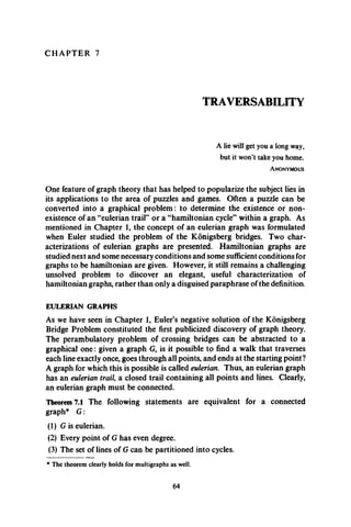
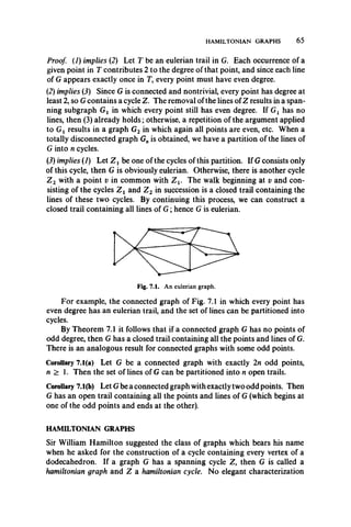
![66 TRAVERSABILITY
of hamiltonian graphs exists, although several necessary or sufficient con
ditions are known.
A theta graph is a block with two nonadjacent points of degree 3 and all
other points of degree 2. Thus a theta graph consists of two points of degree
3 and three disjoint paths joining them, each of length at least 2.
Theorem 7.2 Every hamiltonian graph is 2-connected. Every nonhamiltonian
2-connected graph has a theta subgraph.
It is easy to find a theta subgraph in the nonhamiltonian block of Fig. 7.2.
The next theorem, due to Posa [P7], gives a sufficient condition for a
graph to be hamiltonian. It generalizes earlier results by Ore and Dirac
which appear as its corollaries.
Theorem 7.3 Let G have p > 3 points. If for every n, 1 < n < (p — l)/2,
the number of points of degree not exceeding n is less than n and if, for odd p,
the number of points of degree at most (p — l)/2 does not exceed (p — l)/2,
then G is hamiltonian.
Proof. Assume the theorem does not hold and let G be a maximal non
hamiltonian graph with p points satisfying the hypothesis of the theorem.
It is easy to see that the addition of any line to a graph satisfying the con
ditions of the theorem results in a graph which also satisfies these conditions.
Thus since the addition of any line to G results in a hamiltonian graph, any
two nonadjacent points must be joined by a spanning path.
We first show that every point of degree at least (p — l)/2 is adjacent
to every point of degree greater than (p — l)/2. Assume (without loss of
generality) that deg > (p — l)/2 and deg vp > p/2, but vx and vp are not
adjacent. Then there is a spanning path vi v2 ' " v p connecting vx and vp.
Let the points adjacent to vx be vil9 • • •, vin where n = deg vx and 2 =
*i < h < ' ** < V Clearly vp cannot be adjacent to any point of G of the
form Vi.-1, for otherwise there would be a hamiltonian cycle
vx v2 ‘ ' vtj—i vp tfp-i **• V^Vi
in G. Now since n > (p — l)/2, we have p/2 < deg vp < p — 1 —n < p/2
which is impossible, so vx and vp must be adjacent.](https://image.slidesharecdn.com/graphtheory-181103155731/85/Graph-theory-77-320.jpg)
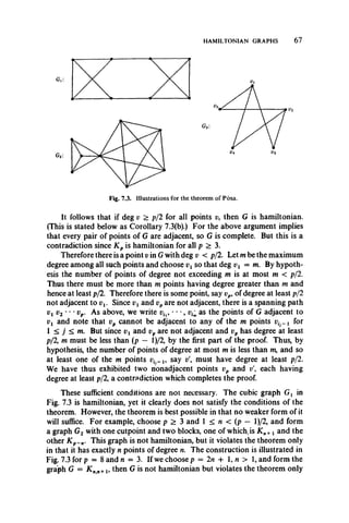
![68 TRAVERSABILITY
by having (p - l)/2 + 1 points of degree (p - l)/2. The graph G3 = K 23
of Fig. 7.3 illustrates this construction for p = 5.
By specializing Posa’s Theorem, we obtain simpler but less powerful
sufficient conditions due to Ore [0 3 ] and Dirac [D6] respectively.
Corollary 7.3(a) If p > 3 and for every pair u and v of nonadjacent points,
deg u + deg v > p, then G is hamiltonian.
Corollary 73(b) If for all points v of G, deg v > p/2, where p > 3, then G is
hamiltonian.
Actually, the cubic hamiltonian graph Gt of Fig. 7.3 has four spanning
cycles. The smallest cubic hamiltonian graph,. K4, has three spanning cycles.
These observations serve to illustrate a theorem of C. A. B. Smith which
appears in a paper by Tutte [T6].
Theorem 7.4 Every cubic hamiltonian graph has at least three spanning
cycles.
Tait [T l] conjectured that every cubic 3-connected planar graph*
contains a spanning cycle. Tutte [T6] settled this in the negative by showing
that the 3-connected planar graph with 46 points ofFig. 7.4 is not hamiltonian.
The smallest known nonhamiltonian triply connected cubic planar graph,
having 38 points, was constructed independently by J. Lederberg, J. Bosak,
and D. Barnette; see Grunbaum [G10, p. 359].
The apparent lack of any relationship between eulerian and hamiltonian
graphs is illustrated in Fig. 7.5 where each graph is a block with eight points.
* See Chapter 11 for a discussion of planarity. Tait’s conjecture, if true, would have settled
the Four Color Conjecture.](https://image.slidesharecdn.com/graphtheory-181103155731/85/Graph-theory-79-320.jpg)
![EXERCISES 69
Hamiltonian Nonhamiltonian
Eulerian
Noneulerian
Fig. 7.5. Eulerian and/or hamiltonian graphs.
However, in the next chapter we shall relate eulerian and hamiltonian
graphs by way of the “line graph.”
Incidentally, M. D. Plummer conjectures that the square of every
2-connected graph is hamiltonian.
EXERCISES
7.1 Find an eulerian trail in the graph G of Fig. 7.1 and a partition of the lines of G
into cycles.
7.2 Ifevery block ofa connected graph Giseulerian, then Gis eulerian, and conversely.
7.3 In Corollary 7.1(a), the partition cannot be done with fewer than n trails. State
and prove the converse of Corollary 7.1(b).
7.4 A graph is arbitrarily traversablefrom a point v0if the following procedure always
results in an eulerian trail: Start at point v0by traversing any incident line;on arriving
at a point u depart by traversing any incident line not yet used, and continue until no
new lines remain.
a) An eulerian graph is arbitrarily traversable from v0 if and only if every cycle
contains v0. (Ore [02])
b) If G is arbitrarily traversable from v0, then v0 has maximum degree.
(Babler [Bl])
c) If G is arbitrarily traversable from v0, then either v0 is the only cutpoint or
G has no cutpoints. (Harary [HI7])
7.5 Prove or disprove: If a graph G contains an induced theta subgraph, then G is
not hamiltonian.
7.6 a) For any nontrivial connected graph G, every pair of points of G3are joined by
a spanning path. Hence every line of G3is in a hamiltonian cycle, when p > 3.
(Karaganis [K2])
b) If every pair of points of G are joined by a spanning path and p > 4, then G
is 3-connected.](https://image.slidesharecdn.com/graphtheory-181103155731/85/Graph-theory-80-320.jpg)
![70 TRAVERSABILITY
7.7 Give an example of a nonhamiltonian graph with 10 points such that for every
pair of nonadjacent points u and v, deg u -f deg v >9.
7.8 How many spanning cycles are there in the complete bigraphs K33 and K4>3?
7.9 A graph G is called randomly traceable [randomly hamiltonian] if a spanning
path [hamiltonian cycle] always results upon starting at any point of G and then
successively proceeding to any adjacent point not yet chosen until no new points are
available.
a) A graph Gwith p > 3 points is randomly traceable if and only if it is randomly
hamiltonian.
b) A graph Gwith p > 3joints is randomly traceable if and only if it is one of the
graphs Cp, Kpi or Knnwith p = 2n. (Chartrand and Kronk [CK1])
7.10 Theorem 7.3 can be regarded as giving sufficient conditions for a graph to be
2-connected. This can be generalized to the n-connected case.
Let G be nontrivial and let 1 < n < p. The following conditions are sufficient
for G to be n-connected:
1. For every k such that n — < k < ( p + n —3)/2, the number of points of
degree not exceeding k does not exceed k + 1 — n.
2. The number of points of degree not exceeding (p + n —3)/2 does not exceed
p —n. (Chartrand, Kapoor, and Kronk [CKK1])
7.11 Posa’s theorem can also be generalized in another way.
Let G have p > 3 and let 0 < k < p - 2. If for every integer i with k + 1 <
i < (p + Ac)/2, the number of points not exceeding i is less than i —k, then every path of
length k is contained in a hamiltonian cycle. (Kronk [K13])
7.12 Recall that two labeled graphsare isomorphic if there is a label-preserving
isomorphism between them. By an e-graph is meant one in which every point has even
degree.
a) The number of labeled graphs with p points is 2p{p~1)/2.
b) The number of labeled e-graphs with p points equals the number of labeled
graphs with p — 1 points. (R. W. Robinson)
7.13 If G is a (p, q) graph with p > 3 and q > (p2 —3p + 6)/2, then G is hamiltonian.
(Ore [04])
7.14 If for any two nonadjacent points u and vof G, deg u + deg v > p -1-1, then there
is a spanning path joining every pair of distinct points. (Ore [06])
7.15 If G is a graph with p > 3 points such that the removal of any set of at most n
points results in a hamiltonian graph, then G is (n -I- 2)-connected.
(Chartrand, Kapoor, Kronk [CKK1])
7.16 Consider the nonhamiltonian graphs G such that every subgraph G — v is
hamiltonian. There is exactly one such graph with 10 points and none smaller.
(Gaudin, Herz, and Rossi [GHR1])
7.17 Do there exist nonhamiltonian graphs with arbitrarily high connectivity?](https://image.slidesharecdn.com/graphtheory-181103155731/85/Graph-theory-81-320.jpg)
![C H A P T E R 8
LINE GRAPHS
A straight line is the shortest distance between two points.
E u c l i d
The concept of the line graph of a given graph is so natural that it has been
independently discovered by many authors. Ofcourse, each gave it a different
name*:Ore [05] calls it the “interchange graph,” Sabidussi [S7] “derivative”
and Beineke [B8] “derived graph,” Seshu and Reed [SRI] “edge-to-vertex
dual,” Kasteleyn [K4] “covering graph,” and Menon [M10] “adjoint.”
Various characterizations of line graphs are developed. We also introduce
the total graph, first studied by Behzad [B4], which has surprisingly been
discovered only once thus far, and hence has no other names. Relationships
between line graphs and total graphs are studied, with particular emphasis
on eulerian and hamiltonian graphs.
SOME PROPERTIES OF LINE GRAPHS
Consider the set X of lines of a graph G with at least one line as a family
of 2-point subsets of V(G). The line graph of G, denoted L(G), is the intersec
tion graph ). Thus the points of L(G) are the lines of G, with two points of
L(G) adjacent whenever the corresponding lines of G are. If x = uv is a line
of G, then the degree of x in L(G) is clearly deg u + deg v — 2. Two exam
ples of graphs and their line graphs are given in Fig. 8.1. Note that in this
figure G2 = L(Gj), so that L(G2) = L(L(GX)). We write Lf(G) = L(G),
L2(G) = L(L(G)), and in general the iterated line graph is E(G) = L(E~ 1(G».
As an immediate consequence of the definition of L(G), we note that
every cutpoint ofL(G) is a bridge of G which is not an endline, and conversely.
When defining any class of graphs, it is desirable to know the number of
points and lines in each; this is easy to determine for line graphs.
* Hoffman [H46J uses “line graph” even though he chooses “edge.” Whitney [W 11] was the
first to discover these graphs but didn’t give them a name.
71](https://image.slidesharecdn.com/graphtheory-181103155731/85/Graph-theory-82-320.jpg)
![7 2 LINE GRAPHS
Fig. 8.1. Graphs and their line graphs.
Theorem 8.1 If G is a (p, q) graph whose points have degrees dh then L(G)
has q points and qL lines, where
Ql = —<1 + t Z d f -
Proof. By the definition of line graph, L(G) has q points. The d{ lines
incident with a point v( contribute (dj) to qLj so
4*. = 1 ( 2) = 414(4 - i) = *!«*? - 4 1 4 = 414? - 9.
The next result can be proved in many different ways, depending on
one’s whimsy.
Theorem 8.2 A connected graph is isomorphic to its line graph if and only
if it is a cycle.
Thus for a (not necessarily connected) graph, G = L(G) if and only if
G is regular of degree 2.
If Gj and G2 are isomorphic, then obviously L(Gi) and L(G2) are.
Whitney [W ll] found that the converse almost always holds by displaying
the only two different graphs with the same line graph. The proof given here
is due to Jung [J3].
Theorem 8.3 Let G and G' be connected graphs with isomorphic line graphs.
Then G and G' are isomorphic unless one is K 3 and the other is K t 3.
Proof First note that among the connected graphs with up to four points,
the only two different ones with isomorphic line graphs are K 3 and K t 3.](https://image.slidesharecdn.com/graphtheory-181103155731/85/Graph-theory-83-320.jpg)
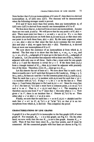
![74 LINE GRAPHS
Since L(C4) = C4 by Theorem 8.3 and L(K l 3 + x) = JC4 — x (see Fig. 8.1),
it follows that H is one of the three trees. But the line graphs of these trees
are the path P 4, the graph K 2• K 2, and K A, showing that K l 3 is not a line
graph. We will see that the star K l 3plays an important role in characterizing
line graphs. The first characterization of line graphs, statement (2) of
the next theorem and due to Krausz [K12], was rather close to the defini
tion. The situation was improved by van Rooij and Wilf [RW1] who were
able to describe in (3) a structural criterion for a graph to be a line graph.
Finally, Beineke [B8] and N. Robertson (unpublished) displayed exactly
those subgraphs which cannot occur in line graphs. Recall that an induced
subgraph is one which is maximal on its point set. A triangle T of a graph G
is called odd if there is a point of G adjacent to an odd number of its points,
and is even otherwise.
Theorem 8.4 The following statements are equivalent:
(1) G is a line graph.
(2) The lines of G can be partitioned into complete subgraphs in such a
way that no point lies in more than two of the subgraphs.
(3) G does not have K x 3 as an induced subgraph, and if two odd triangles
have a common line then the subgraph induced by their points is AT4.
(4) None of the nine graphs of Fig. 8.3 is an induced subgraph of G.
Proof. (1) implies (2) Let G be the line graph of H. Without loss of generality
we assume that H has no isolated points. Then the lines in the star at each
point of H induce a complete subgraph of G, and every line of G lies in exactly
one such subgraph. Since each line of H belongs to the stars of exactly
two points of //, no point of G is in more than two of these complete
subgraphs.
(2) implies (1) Given a decomposition of the lines of a graph G into complete
subgraphs Sj, S2, • • •, Sn satisfying (2), we indicate the construction of a
graph H whose line graph is G. The points of H correspond to the se( S of](https://image.slidesharecdn.com/graphtheory-181103155731/85/Graph-theory-85-320.jpg)
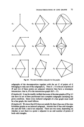
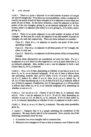
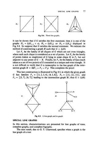
![78 LINE GRAPHS
Theorem 8.5 A graph is the line graph of a tree if and only if it is a connected
block graph in which each cutpoint is on exactly two blocks.
Proof, Suppose G = L(T),T some tree. Then G is also B(T) since the lines
and blocks of a tree coincide. Each cutpoint x of G corresponds to a bridge
uv of T, and is on exactly those two blocks of G which correspond to the
stars at u and v. This proves the necessity of the condition.
To see the sufficiency, let G be a block graph in which each cutpoint is
on exactly two blocks. Since each block of a block graph is complete, there
exists a graph H such that L(H) = G by Theorem 8.4. If G = K 3, we can
take H = K l 3. If G is any other block graph, then we show that H must be
a tree. Assume that H is not a tree so that it contains a cycle. If H is itself
a cycle, then by Theorem 8.2, L(H) = H, but the only cycle which is a block
graph is X 3, a case not under consideration. Hence H must properly contain
a cycle, thereby implying that H has a cycle Z and a line x adjacent to two
lines of Z, but not adjacent to some line y of Z. The points x and y of L(H)
lie on a cycle of L(//), and they are not adjacent. This contradicts the
condition of Theorem 3.5 that L(H) is a block graph. Hence H is a tree, and
the theorem is proved.
In Fig. 8.6, a block graph G is shown in which each cutpoint lies on just
two blocks. The tree T of which G is the line graph is constructed by first
forming the block graph B(G) and then adding new points for the non-
cutpoints of G and the lines joining each block with its noncutpoints.
The line graphs of complete graphs and complete bigraphs are almost
always characterized by rather immediate observations involving adjacencies
of lines in K p and K m„. The case of complete graphs was independently
settled by Chang [C 7]’and Hoffman [H43], [H44].](https://image.slidesharecdn.com/graphtheory-181103155731/85/Graph-theory-89-320.jpg)
![LINE GRAPHS AND TRAVERSABILITY 79
Theorem 8.6 Unless p = 8, a graph G is the line graph of Kp if and only if
1. Ghas(£) points,
2. G is regular of degree 2(p — 2),
3. Every two nonadjacent points are mutually adjacent to exactly four
points,
4. Every two adjacent points are mutually adjacent to exactly p — 2
points.
It is evident that L(Kp) has these four properties. It is not at all obvious
that when p = 8, there are exactly three exceptional graphs satisfying the
conditions.
For complete bigraphs, the corresponding result was found by Moon
[M l3], and Hoffman .[H46].
Theorem 8.7 Unless m = n = 4, a graph G is the line graph of K mn if and
only if
1. G has mn points,
2. G is regular of degree m 4- n — 2,
3. Every two nonadjacent points are mutually adjacent to exactly two
points,
4. Among the adjacent pairs of points, exactly n(2) pairs are mutually
adjacent to exactly m — 2 points, and the other m(2) pairs to n — 2
points.
There is only one exceptional graph satisfying these conditions. It has
16 points, is not L(K4 4), and was found by Shrikhande [SI2] when he
proved Theorem 8.7 for the case m = n.
LINE GRAPHS AND TRAVERSABILITY
We now investigate the relationship of eulerian and hamiltonian graphs
with line graphs.
If x = uv is a line of G, and w is not a point of G, then x is subdivided
when it is replaced by the lines uw and wv. If every line of G is subdivided, the
Fig. 8.7. A graph and its subdivision graph.](https://image.slidesharecdn.com/graphtheory-181103155731/85/Graph-theory-90-320.jpg)
![80 LINE GRAPHS
L(G)
Fig. 8.9. Another counterexample.
resulting graph is the subdivision graph 5(G); see Fig. 8.7. If we denote by
5„(G) the graph obtained from G by inserting n new points of degree 2 into
every line of G, so that 5(G) = 5 t(G), we can then define a new graph
L„(G) = L(5b_j(G)). Note that, in general, Ln(G) qk ZT(G), the nth iterated
line graph of G.
Theorem 8.8 If G is eulerian, then L(G) is both eulerian and hamiltonian. If
G is hamiltonian, then L(G) is hamiltonian.
It is easy to supply counter-examples to the converses ofthese statements.
For example in Fig. 8.8, L(G) is eulerian and hamiltonian while G is not
eulerian; in Fig. 8.9, L(G) is hamiltonian while G is not.
A refinement of the second statement in Theorem 8.8 is provided by the
following result of Harary and Nash-Williams [HN1] which follows readily
from the preceding theorem and the fact that L2(G) = L(S(G)).
Theorem 8.9 A sufficient condition for L2(G) to be hamiltonian is that G
be hamiltonian and a necessary condition is that L(G) be hamiltonian.
The graphs of Figs. 8.10 and 8.9 show that the first of these conditions
is not necessary and the second is not sufficient for L2(G) to be hamiltonian.
We note also (see Fig. 8.11) that L(G) = L^G) and L2(G) may be hamiltonian](https://image.slidesharecdn.com/graphtheory-181103155731/85/Graph-theory-91-320.jpg)
![LINE GRAPHS AND TRAVERSABILITY 81
Fig. 8.10. Still another counterexample.
L(G)
Fig. 8.11. A sequence of graphs Ln(G).
without G being eulerian. However, the next graph L3(G) in this series
provides the link between these two properties.
Theorem 8.10 A graph G is eulerian if and only if L3(G) is hamiltonian.
For almost every connected graph G, however, nearly all of the graphs
12(G) are hamiltonian, as shown by Chartrand [C9].
Theorem 8.11 If G is a nontrivial connected graph with p points which is not
a path, then 12(G) is hamiltonian for all n > p — 3.
An example is given in Fig. 8.12 in which a 6-point graph G, as well as
L(G), L2(G), and the hamiltonian graph L3(G) are shown.
L(G) LHG)
Fig. 8.12. A sequence of iterated line graphs.
LHG)](https://image.slidesharecdn.com/graphtheory-181103155731/85/Graph-theory-92-320.jpg)
![82 LINE GRAPHS
TOTAL GRAPHS
The points and lines of a graph are called its elements. Two elements of a
graph are neighbors if they are either incident or adjacent. The total graph
T(G) has point set V(G) u X(G and two points of T(G) are adjacent whenever
they are neighbors in G. Figure 8.13 depicts the formation of the total
graph T(K 3). It is easy to see that T(G) always contains both G and L(G) as
induced subgraphs.
An alternative characterization of total graphs was given by Behzad
[B4].
Theorem 8.12 The total graph T(G) is isomorphic to the square of the sub
division graph 5(G).
Corollary 8.12(a) If v is a point of G, then the degree of point v in T(G) is
2 deg v. If x = uv is a line of G, then the degree of point x in T(G) is
deg u + deg v.
Corollary 8.12(b) If G is a (p, q) graph whose points have degrees dh then the
total graph T(G) has pT = p -f q points and qT = 2q + ^ £ df lines.
The Ramsey function r(m, n) was defined in Chapter 2, where it was noted
that its general determination remains an unsolved problem. Behzad and
Radjavi [BR1] defined and solved an analogue of the Ramsey problem,
suggested by line graphs. The line Ramsey number r^m, n) is the smallest
positive integer p such that every connected graph with p points contains
either n mutually disjoint lines or m mutually adjacent lines, that is, the star
K l m. Thus r^m, n) is the smallest integer p such that for any graph G
with p points, L(G) contains K mor L(G) contains K„.
Theorem 8.13 For n > 1, we always have rj(2, n) = 3. For all other m and w,
rj(m, ri) = (m — l)(n - 1) 4- 2.
Note that it is not always true that rt(m, n) = rt(n, m). Furthermore,
in contrast with Ramsey numbers, r^m^n) is defined only for connected
graphs.](https://image.slidesharecdn.com/graphtheory-181103155731/85/Graph-theory-93-320.jpg)
![EXERCISES 83
EXERCISES
8.1 Under what conditions can the lines of a line graph be partitioned into complete
subgraphs so that each point lies in exactly two of these subgraphs?
8.2 Determine the number of triangles in L(G) in terms of the number n of triangles of
Gand the partition of G.
8.3 Determine a criterion for a connected graph to have a regular line graph.
8.4 A graph G can be reconstructed from the collection of q spanning subgraphs
G - Xj if and only if its line graph L(G) satisfies Ulam’s Conjecture (p. 12).
(Hemminger [H41])
8.5 If G is n-line-connected, then
1. L(G) is n-connected,
2. L(G) is (2n —2)-line-connected, and
3. L2(G) is (2n —2)-connected. (Chartrand and Stewart [CS1])
8.6 a) Construct a connected graph G with p > 4 such that L(G) is not eulerian but
13(G) is.
b) There is no connected graph G with p > 5 such that L2(G) is not eulerian and
13(G) is.
8.7 The smallest block whose line graph is not hamiltonian is the theta graph with
8 points in which the distance between the points of degree 3 is 3. (J. W. Moon)
8.8 L(G) is hamiltonian if and only if there is a closed trail in G which includes at
least one point incident with each line of G.
8.9 The graph L2(G) is hamiltonian if and only if G has a closed spanning trail.
(Harary and Nash-Williams [HN1])
8.10 The following statements are equivalent
(1) L(G) is eulerian.
(2) The degrees of all the points of G are of the same parity and G is connected.
(3) T(G) is eulerian.
8.11 T(Kp) is isomorphic to L(Xp+j). (Behzad, Chartrand, and Nordhaus [BCN1])
8.12 Define a family F of subsets of elements of G such that T(G) = Q(F).
8.13 a) If G is hamiltonian, so is T(G). If G is eulerian, then T(G) is both eulerian and
hamiltonian.
b) The total graph T(G)ofevery nontrivial connected graph Gcontains a spanning
eulerian subgraph.
c) If a nontrivial graph G contains a spanning eulerian subgraph, then T(G) is
hamiltonian.
d) If G is nontrivial and connected, then T2(G) is hamiltonian.
(Behzad and Chartrand [BC2])](https://image.slidesharecdn.com/graphtheory-181103155731/85/Graph-theory-94-320.jpg)
![C H A P T E R 9
FACTORIZATION
The whole is equal to the sum of its parts.
E u c l i d , Elements
The whole is greater than the sum of its parts.
M a x W e r t h e i m e r , Productive Thinking
A problem which occurs in varying contexts is to determine whether a given
graph can be decomposed into line-disjoint spanning subgraphs possessing
a prescribed property. Most frequently, this property is that of regularity
of specified degree. In particular, a criterion for the existence in a graph of a
spanning regular subgraph of degree 1 was found by Tutte. Some observa
tions are presented concerning the decomposition of complete graphs into
spanning subgraphs regular of degree 1 and 2.
The partitioning of the lines of a given graph into spanning forests is
also studied and gives rise to an invariant known as “arboricity.” A formula
for the arboricity of a graph in terms of its subgraphs was derived by Nash-
Williams, and explicit constructions for the minimum number of spanning
forests in complete graphs and bigraphs have been devised.
1-FACTORIZATION
Afactor of a graph G is a spanning subgraph of G which is not totally dis
connected. We say that G is the sum* of factors Gf if it is their line-disjoint
union, and such a union is called afactorization of G. An n-factor is regular of
degree n. If G is the sum of n-factors, their union is called an n-factorization
and G itself is n-factorable. Unless otherwise stated, the results presented in
this chapter appear in or are readily inferred from theorems in Konig
[K10, pp. 155-195], where the topic is treated extensively.
When G has a 1-factor, say Gu it is clear that p is even and the lines of Gt
are point disjoint. In particular, K 2n+1 cannot have a 1-factor, but K ln
certainly can.
* Some call this product; others direct sum.
84](https://image.slidesharecdn.com/graphtheory-181103155731/85/Graph-theory-95-320.jpg)
![1-FACTORIZATION 85
Vs v4
G2:
C3: G4:
Fig. 9.1. A 1-factorization of K6.
Theorem 9.1 The complete graph K ln is 1-factorable.
Proof. We need only display a partition of the set X of lines of K ln into
(2n — 1) 1-factors. For this purpose we denote the points of G by
Vu v2>' ' ' >v2n> and define, for i = 1, 2, • • •, 2n — 1, the sets of lines
X { = {ViV2n} u {Vi-pi+J;j = 1, 2, • • •, n - 1}, where each of the subscripts
i —j and i 4- j is expressed as one of the numbers 1, 2, • • •, (2n — 1) modulo
(2n — 1). The collection {X,} is easily seen to give an appropriate partition
of X , and the sum of the subgraphs G, induced by X, is a 1-factorization of
*2„.
For example, consider the graph K 6 shown in Fig. 9.1. The 1-factoriza
tion presented in the proof of the theorem produces the five 1-factors Gf.
Although the complete bigraphs K mn have no 1-factor if m # n, the
graphs Knnare 1-factorable, as seen by the next statement.
Theorem 9.2 Every regular bigraph is 1-factorable.
It is not an easy problem to determine whether a given graph is 1-
factorable, or, indeed, to establish whether there exists any 1-factor. Beineke
and Plummer [BP2] have shown, however, that many graphs cannot have
exactly one 1-factor.
Theorem 9.3 If a 2-connected graph has a 1-factor, then it has at least two
different 1-factors.
The graph G in Fig. 9.2 is a block with exactly two 1-factors, and they
have one common line.
The most significant result on factorization is due to Tutte [T7] and
characterizes graphs possessing a 1-factor. In general, this test for a 1-factor
is quite inconvenient to apply. The proof given here is based on Gallai [G I].](https://image.slidesharecdn.com/graphtheory-181103155731/85/Graph-theory-96-320.jpg)
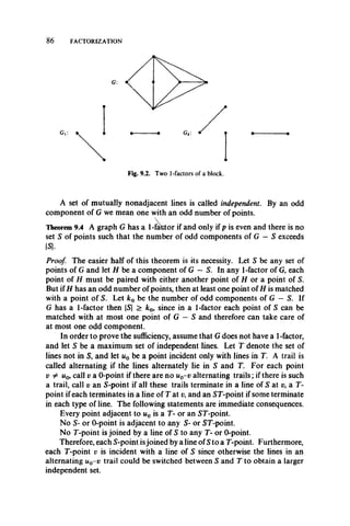
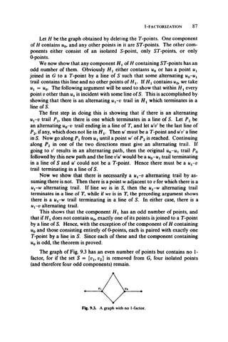
![88 FACTORIZATION
Building up on his criterion for the existence of a 1-factor in a given
graph, Tutte [T10] was able to characterize those graphs having a spanning
subgraph with prescribed degree sequence, and later, [T il], proved this
result as a straightforward consequence of Theorem 9.4. Consider a labeling
of G and a function / from V into the nonnegative integers. Let S and
T be disjoint subsets of V, let H be a component of G —(S u T), and let
q(H, T) be the number of lines of G joining a point of H with one in T. Then
we may write fc0(S, T) as the number of components H of G — (S u T)
sue h that q(H, T ) + ZMeW/ (m) is odd.
Theorem 9.5 Let G be a given graph and let / be a function from V into the
nonnegative integers. Then G has no spanning subgraph whose degree se
quence is prescribed by / if and only if there exist disjoint sets S and T of
points such that
2-FACTORIZATION
If a graph is 2-factorable, then each factor must be a union of disjoint cycles.
If a 2-factor is connected, it is a spanning cycle. We saw that a complete
graph is 1-factorable if and only if it has an even number of points. Since
a 2-factorable graph must have all points even, the complete graphs K 2n
are not 2-factorable. The odd complete graphs are 2-factorable, and in
fact a stronger statement can be made.
! / ( « ) < k0(S, T) + £[/(!>) - dG^ v ) l
Fig. 9.4. A 2-factorization of K-,.](https://image.slidesharecdn.com/graphtheory-181103155731/85/Graph-theory-99-320.jpg)
![2 -f a c t o r iz a t io n 89
Theorem 9.6 The graph K 2n+1 is the sum of n spanning cycles.
Proof. In order to construct n line-disjoint spanning cycles in K 2n+1, first
label its points vu v2, • • •, v2n+j. Then construct n paths Pt on the points
Vi,v2, ' ’ -,v 2„as follows: P, = vi vi_l vi+1 y,_2 • vi+m_ i Thus the ;th
point of Pi is vk, where k = i + (—l)J+1[y/2] and all subscripts are
taken as the integers 1, 2, • • •, 2n (mod 2n). The spanning cycle Z xis then
constructed by joining v2n+x to the endpoints of Pf.
This construction is illustrated in Fig. 9.4 for the graph K n. The lines
of the paths P* are solid and the two added lines are dashed.
There is a decomposition of K 2nwhich embellishes the result of Theorem
9.1.
Theorem 9.7 The complete graph K 2n is the sum of a 1-factor and n — 1
spanning cycles.
Of course, every regular graph of degree 1 is itself a 1-factor and every
regular graph of degree 2 is a 2-factor. If every component of a regular
graph G of degree 2 is an even cycle, then G is also 1-factorable since it can
be expressed as the sum of two 1-factors. If a cubic graph contains a 1-factor,
it must also have a 2-factor, but there are many cubic graphs which do not
have 1-factors.
The graph of Fig. 9.5 has three bridges. Petersen [P3] proved that any
cubic graph without a 1-factor must have a bridge.
Theorem 9.8 Every bridgeless cubic graph is the sum of a 1-factor and a
2-factor.
Petersen showed that this result could not be strengthened by exhibiting
a bridgeless cubic graph which is not the sum of three 1-factors. This well-
known graph, shown in Fig. 9.6, is called the Petersen graph. By Theorem 9.8,
it is the sum of a 1-factor and a 2-factor. The pentagon and pentagram
together constitute a 2-factor while the five lines joining the pentagon with
the pentagram form a 1-factor.](https://image.slidesharecdn.com/graphtheory-181103155731/85/Graph-theory-100-320.jpg)
![9 0 FACTORIZATION
A criterion for the decomposability of a graph into 2-factors was also
obtained by Petersen [P3].
Theorem 9.9 A graph is 2-factorable if and only if it is regular of even degree,
even degree.
ARBORICITY
In the only type of factorization considered thus far, each factor has been
an H-factor. Several other kinds of factorizations have been investigated
and we discuss one now and others in Chapter 11. Any graph G can be
expressed as a sum of spanning forests, simply by letting each factor contain
only one of the q lines of G. A natural problem is to determine the minimum
number of line-disjoint spanning forests into which G can be decomposed.
This number is called the arboricity of Gand is denoted by Y(G). For example,
T(X4) = 2 and Y(K s) = 3; minimal decompositions of these graphs into
spanning forests are shown in Fig. 9.7.
A formula discovered by Nash-Williams [N2] gives the arboricity of
any graph.
Theorem 9.10 Let G be a nontrivial (p, q) graph and let qn be the maximum
number of lines in any subgraph of G having n points. Then
The fact that Y(G) > max,, {qj(n - 1)} can be shown as follows.
Since G has p points, the maximum number of lines in any spanning forest
is p — 1. Hence, the minimum possible number of spanning forests required
Fig. 9.7. Minimal decompositions into spanning forests.](https://image.slidesharecdn.com/graphtheory-181103155731/85/Graph-theory-101-320.jpg)
![ARBORICITY 91
to fill G, which by definition is Y(G), is at least q/(p — 1). But the arboricity
ofG is an integer, so Y(G) > {q/(p — 1)}. The desired inequality now follows
from the fact that for any subgraph H of G, Y(G) > Y(H).
Among all subgraphs H with n < p points, max Y(H) will occur in those
induced subgraphs containing the greatest number of lines. Thus if H is a
subgraph of G, Y(H) can be greater than {q/{p - 1)}. The (10, 15) graph in
Fig. 9.8 illustrates this observation. Takings = 5and<?rt = 10 (for H = K s),
we have
For Kp9the maximum value of qj(n — 1) clearly occurs for n = p so that
Y(Kp) = {p/2}. Similarly, for the complete bigraph K rs, {qj{n - 1)}
assumes its maximum value when n = p = r + s.
Corollary 9.10(a) The arboricities of the complete graphs and bigraphs are
T(K, ) - { ? } and Y(K,,,) . .
Although Nash-Williams’ formula gives the minimum number of
spanning forests into which an arbitrary graph can be factored, his proof
does not display a specific decomposition. Beineke [B5] accomplished this
for complete graphs and bigraphs, the former of which we present here. For
p = 2n, K pcan actually be decomposed into n spanning paths. Labeling the
points vl9 v2, ' , v2ni we consider the same n paths
Pi = Vi !>(_, vi+l rf_2 vi+2 ■■■ V i _ n,
as in proof of Theorem 9.6. For p = 2n + 1, the arboricity of K p is n + 1
by Corollary 9.10(a). A decomposition is obtained by taking the paths just
described, adding an extra point labeled v2n+1 to each, and then constructing](https://image.slidesharecdn.com/graphtheory-181103155731/85/Graph-theory-102-320.jpg)
![92 FACTORIZATION
Fig. 9.9. A minimal decomposition of Kq into spanning forests.
a star by joining v2n+ 1 to the other 2n points. The construction for p = 9
is shown in Fig. 9.9. It is easily seen to consist of the star at one of the points
of K g together with spanning subforests corresponding to the four spanning
paths of K 8 indicated above.
EXERCISES
9.1 The graph K4 has a unique 1-factorization. Find the number of 1-factorizations
of K33 and of K6.
9.2 Display a 1-factorization for K%.
9.3 The number of 1-factors in K2nis (2n)!/(2"n!).
9.4 K6n_2has a 3-factorization.
9.5 Forn > 1, X4n+1 is 4-factorable.
9.6 Use Tutte’s Theorem 9.4 to show that the graph of Fig. 9.5 has no 1-factor.
9.7 If an n-connected graph G with p even is regular of degree n, then G has a 1-factor.
(Tutte [T7])
9.8 Prove or disprove: Let G be a graph with a 1-factor F. A line of G is in more than
one 1-factor if and only if it lies on a cycle whose lines are alternately in F.
(Beineke and Plummer [BP2])
9.9 Express Kgas the sum of four spanning cycles.
9.10 Is the Petersen graph hamiltonian?](https://image.slidesharecdn.com/graphtheory-181103155731/85/Graph-theory-103-320.jpg)
![EXERCISES 93
*9.11 Corresponding to any two integers d > 3 and g > 3, there exists a graph G with
the following properties:
1. G is regular of degreed.
2. G has girth g.
3. G is hamiltonian.
4. The cycles of length g are line-disjoint and constitute a 2-factor of G.
5. G is the sum of this 2-factor and (d —2) 1-factors. (Sachs [S9])
9.12 Display a minimal decomposition of K4A into spanning forests.
9.13 Find the smallest connected (p, q) graph G such that
max, {qr/(r - 1)} > {q/(p - 1)},
where qr is the maximum number of lines in any induced subgraph of G with r points.](https://image.slidesharecdn.com/graphtheory-181103155731/85/Graph-theory-104-320.jpg)
![C H A P T E R 10
COVERINGS
Through any point not on a given line, there passes
a unique line having no points in common with the given line.
E u c l i d
Through any point not on a given line, there passes
no line having no points in common with the given line.
R ie m a n n
Through any point not on a given line, there pass
more than one line having no points in common with the given line.
B o l y a i
It is natural to say that a line x = uv of G covers the points u and v. Similarly,
we may consider each point as covering all lines incident with it. From this
viewpoint, one defines two invariants of G : the minimum number of points
(lines) which cover all the lines (points). Two related invariants are the
maximum number of nonadjacent points and lines. These four numbers
associated with any graph satisfy several relations and also suggest the study
of special points and lines which are critical for covering purposes. These
concepts lead naturally to two special subgraphs of G called the line-core
and point-core. Criteria for the existence of such subgraphs are established
in terms of covering properties of the graph.
COVERINGS AND INDEPENDENCE
A point and a line are said to cover each other if they are incident. A set of
points which covers all the lines of a graph G is called a point cover for G,
while a set of lines which covers all the points is a line cover. The smallest
number of points in any point cover for G is called its point covering number
and is denoted by a0(G) or a0. Similarly, a^G) or <x{ is the smallest number of
lines in any line cover of G and is called its line covering number. For example,
oc0(Kp) = p — 1 and olx(Kp) = [(p + l)/2]. A point cover (line cover) is
called minimum if it contains a0 (respectively o^) elements. Observe that a
94](https://image.slidesharecdn.com/graphtheory-181103155731/85/Graph-theory-105-320.jpg)
![COVERINGS AND INDEPENDENCE 9 5
Fig. 10.1. The graph K4 ■K4.
point cover may be minimal without being minimum; such a set of points
is given by the 6 noncutpoints in Fig. 10.1. The same holds for line covers;
the 6 lines incident with the cutpoint serve.
A set of points in G is independent if no two of them are adjacent. The
largest number of points in such a set is called the point independence number
of G and is denoted by P0(G) or j30. Analogously, an independent set of lines
of G has no two of its lines adjacent and the maximum cardinality of such a
set is the line independence number P X(G) or p x. For the complete graph,
Po(Kp) = lan d Pi(Kp) = [p/2]. Obviously P f G ) = p/2 if and only if G has
a 1-factor. The numbers just defined are P0(G) = 2 and p x(G) = 3 for the
graph G of Fig. 10.1.
For this graph as well as for Kp,a 0 + /?o = a i + /?i = P- Gallai [G2]
proved that this identity always holds.
Theorem 10.1 For any nontrivial connected graph G,
«o + Po = P = <*i + Pi-
Proof. Let M 0be any maximum independent set ofpoints, so that M0 = p0.
Since no line joins two points of Af0, the remaining set of p — P0 points
constitutes a point cover for G so that a0 < p —p0. On the other hand,
if N 0 is a minimum point cover for G, then no line can join any two of the
remaining p —a0 points of G, so the set V — N 0 is independent. Hence,
Po > p — a0, proving the first equation.
To obtain the second equality, we begin with an independent set M x of
Pl lines. A line cover Y is then produced by taking the union of M x and a
set of lines, one incident line for each point of G not covered by any line
in M v Since M X + |T| < p and Y > a 1? it follows that <xl + p x < p.
In order to show the inequality in the other direction, let us consider a
minimum line cover N xof G. Clearly, N xcannot contain a line both of whose
endpoints are incident with lines also in N x. This implies that N x is the sum
of stars of G (considered as sets of lines). If one line is selected from each of
these stars, we obtain an independent set W of lines. Now, N X + W = p
and W < px thus, olx + p x > p, completing the proof of the theorem.](https://image.slidesharecdn.com/graphtheory-181103155731/85/Graph-theory-106-320.jpg)
![9 6 COVERINGS
Hedetniemi [H39] noticed that the proof of the first equation in
Theorem 10.1,
a0 + Po = A
applies in a more general setting. A property P of a graph G is hereditary
if every subgraph of G also has this property. Examples of hereditary
properties include a graph being totally disconnected, acyclic, and bipartite.
A set S ofpoints of G is called a jP-set ifthe induced subgraph <S> has property
P ; it is called a P-set if every subgraph of G without property P contains a
point of S. Let fi0(P) be the maximum cardinality of a P-set of G and let
a0(P) be the minimum number of points of a P-seL Then the proof of the
next statement is obtained at once from that of Theorem 10.1.
Corollary 10.1(a) If P is an hereditary property of G, then a0(P) + fi0(P) = p.
A collection of independent lines of a graph G is sometimes called a
matching of G since it establishes a pairing ofthe points incident to them. For
this reason, a set of independent lines in G iscalled a maximum matchingofG.
If G is bipartite, then more can be said. The next theorem due to Kdnig [K9]
is intimately related to his Theorem 5.18 on systems ofdistinct representatives
stated in matrix form, in fact it is the same result.
Theorem 10.2 If G is bipartite, then the number of lines in a maximum
matching equals the point covering number, that is, pt = a0.
The problem of finding a maximum matching, the so-called matching
problem, is closely related to that of finding a minimum point cover.
Let M cz X(G) be a matching of G. In an alternating M-trail, exactly
one of any two consecutive lines is in M. An augmenting M-trail is an
alternating M-trail whose endpoints are not incident with any line of M.
Such a trail must be a path or cycle because M is a matching. If G has no
augmenting M-trail, then matching M is unaugmentable. Clearly every
maximum matching is unaugmentable; the converse is due to Berge [BIO]
and the proof given below appears in Norman and Rabin [NR1].
Theorem 103 Every unaugmentable matching is maximum.
Proof. Let M be unaugmentable and choose a maximum matching M ' for
which |M — M'|, the number of lines which are in M but not in M', is
minimum. If this number is zero then M = M'. Otherwise, construct a
trail W of maximum length whose lines alternate in M — M' and M'. Since
M' is unaugmentable, trail W cannot begin and end with lines ofM — M ' and
has equally many lines in M — M' and in M'. Now we form a maximum
matching N from M' by replacing those lines of W which are in M ' by the lines
of W in M — M'. Then |M — N < |M - M'|, contradicting the choice of
M' and completing the proof.](https://image.slidesharecdn.com/graphtheory-181103155731/85/Graph-theory-107-320.jpg)
![CRITICAL POINTS AND LINES 9 7
Norman and Rabin [NR1] developed an algorithm, based on the next
theorem, for finding all minimum line covers in a given graph. Let Y be a
line cover of G. An alternating 7-walk is a 7-reducing walk if its endlines
are in 7 and its endpoints are incident to lines of 7 which are not endlines of
the walk. Obviously every minimum line cover has no reducing walk.
Theorem 10.4 If 7 is a line cover of G such that there is no 7-reducing walk,
then 7 is a minimum line cover.
The cover invariants a0 and a1of G refer to the number of points needed
to cover all the lines and vice versa. We may also regard each point as
covering itself and two points as covering each other if they are adjacent, and
similarly for lines. Then other invariants suggest themselves.
Let a00 be the minimum number of points needed to cover V, and let
(Xqo be the minimum number* of independent points which cover V. Then
both these numbers are defined for any graph. Let ocxj and ol x have similar
meanings for the covering of lines by lines. The relationships among these
invariants were determined by Gupta [G il].
Theorem 10.5 For any graph G,
&oo ^ <*oo and a u = a'n .
CRITICAL POINTS AND LINES
Obviously, if H is a subgraph of G, then a0(H) < a0(G). In particular, this
inequality holds when H = G — v or H = G — x for any point v or line x.
If a0(G — v) < a0(G), then v is called a criticalf point ; if a0(G — x) < a0(G),
then x is a critical line of G. Clearly, if v and x are critical, it follows that
a0(G — v) = a0(G —x) = a0 — 1. Critical points are easily characterized.
Theorem 10.6 A point v is critical in a graph G if and only if some minimum
point cover contains v.
Proof. If M is a minimum point cover for G which contains v, then M — {v}
covers G — v; hence, a0(G — v) < M — (p}| = |Af| — 1 = a0(G) — 1 so
that v is critical in G.
Let v be a critical point of G and consider a minimum point cover M'
for G — v. The set M' u {p} is a point cover for G, and since it contains one
more element than Af', it is minimum.
If the removal of a line x = uv from G decreases the point covering
number, then the removal of u or v must also result in a graph with smaller
point covering number. Thus, if a line is critical both its endpoints are
* Berge [B12] calls a00 the “external stability number” and /?0 the “internal stability number”
t In this chapter, “critical” refers to covering; in Chapter 12, the same word will involve coloring.
The meanings should be clear by context.](https://image.slidesharecdn.com/graphtheory-181103155731/85/Graph-theory-108-320.jpg)
![98 COVERINGS
critical. If a graph has critical points, it need not have critical lines; for
example, every point of C4 is critical but no line is.
A graph in which every point is critical is called point-critical while one
having all lines critical is line-critical Thus a graph G is point-critical if and
only if each point of G lies in some minimum point cover for G. From our
previous remarks, every line-critical graph without isolated points is point-
critical. Among the line-critical graphs are the complete graphs, the cycles of
odd length, and the graphs of Fig. 10.2.
A constructive criterion for line-critical graphs is not known at present;
however, the first two corollaries to the following theorem of Beineke,
Harary, and Plummer [BHP1] place some rather stringent conditions on
such graphs.
Theorem 10.7 Any two adjacent critical lines of a graph lie on an odd cycle.
Corollary 10.7(a) Every connected line-critical graph is a block in which any
two adjacent lines lie on an odd cycle.
Theorem 10.7 was derived by generalizing the next result due to Dulmage
and Mendelsohn [DM1].
Corollary 10.7(b) Any two critical lines of a bipartite graph are independent.
LINE-CORE AND POINT-CORE
The line-core* CX(G) of a graph G is the subgraph of G induced by the union
of all independent sets Y of lines (if any) such that | Y — a0(G). This concept
was introduced by Dulmage and Mendelsohn [DM1], who made it an
integral part of their theory of decomposition for bipartite graphs. It is not
always the case that a graph has a line-core, though by Theorem 10.2, every
bipartite graph which is not totally disconnected has one. As an example of
a graph with no line-core, consider an odd cycle Cp. Here we find that
ao(CP) — (P + l)/2 but that Pi(Cp) = (p — l)/2, so Cp has no line-core.
* Called “core” in [DM1] and [HP 19].](https://image.slidesharecdn.com/graphtheory-181103155731/85/Graph-theory-109-320.jpg)
![LINE-CORE AND POINT-CORE 9 9
G: ♦------- < C'&y
V 7
Fig. 10.3. A graph and its line-core.
Harary and Plummer [HP 19] developed a criterion for a graph to have a
line-core. A minimum point cover Af for a graph G with point set V is said to
be external if for each subset Af' of Af, |Af'| < U(M'), where l/(Af') is the
set of all points of V — Af which are adjacent to a point of Af'.
Theorem 10.8 The following are equivalent for any graph G :
(1) G has a line-core.
(2) G has an external minimum point cover.
(3) Every minimum point cover for G is external.
As an example, consider the graph G of Fig. 10.3. This graph has two
minimum point covers: M x = {v2, v5, v6} and Af2 = {v2, v5, p7}. Let us
concentrate on M x. If M = M u then U{M) = {t^, p3, p4, p7}. For
Af'J = {p5, p6}, G(Afi) = {p3, p4, p7}. We observe that M < U(M) and
M < |L/(Afi)|, a fact which is true for every subset of M x hence, by
definition, M x is external. Obviously, M 2 is also external.
On the other hand, there are graphs which are equal to their line-core.
This family of graphs is characterized in the next theorem, given in [HP19].
Following the terminology of Dulmage and Mendelsohn [DM1], we
consider a bigraph G whose point set V is the disjoint union S u T. We say
that G is semi-irreducible if G has exactly one minimum point cover M and
either Af n S or Af n T is empty. Next, G is irreducible if it has exactly two
minimum point covers Afj and Af2and either Afj n S = <£andAf2 n T = (f)
or Afx n T = <f>and M 2 n 5 = 0. Finally, G is reducible if it is neither
irreducible nor semi-irreducible.
G2:
Fig. 10.4. A semi-irreducible and an irreducible graph.](https://image.slidesharecdn.com/graphtheory-181103155731/85/Graph-theory-110-320.jpg)
![100 COVERINGS
Theorem 10.9 A graph G and its line-core Cj(G) are equal if and only if G is
bipartite and not reducible.
Consider the bigraphs Gx and G2 of Fig. 10.4. In Gl9 let S x = {v3, v6}
and Ti = {vu v2, v4, v5, vn}. The bigraph Gx has the unique minimum point
cover Mj = {v3, r6}, and since M x n Tx = </>, Gx is semi-irreducible and
hence equals its line-core. In G2, set S2 = {ul9 w4, u5} and T2 = {u2, u3, u6}.
There are two minimum point covers, namely, M 2 = {u1? u4, u5} and
N 2 = {u2, w3, m6}. However, Af2 n T2 = </> and N2 n S2 = </>; therefore,
G2 is irreducible and also equals its line-core.
EXERCISES
10.1 Prove or disprove: Every point cover of a graph G contains a minimum point
cover.
10.2 Prove or disprove: Every independent set of lines is contained in a maximum
independent set of lines.
10.3 For any graph G, a0(G) > /MG) and <xt(G) > p0(G).
10.4 Find a necessary and sufficient condition that at(G) = /MG).
10.5 If G has a closed trail containing a point cover, then L(G) is hamiltonian.
10.6 For any graph G, a0(G) > £(G).
10.7 If Gis a bigraph then q < a0p0, with equality holding only for complete bigraphs.
10.8 If G is a complete n-partite graph, then
a) a0 = S = k —L
b) G is hamiltonian if and only if p < 2<x0.
c) If G is not hamiltonian, then its circumference c = 2a0 and G has a unique
minimum point cover. (M.D. Plummer)
d) px = min {<5, [p/2]}. (Chartrand, Geller, Hedetniemi [CGH2])
10.9 a) Let PKbe the maximum number of points in a set S c: V(G) such that <S> is
disconnected. Then k —p — PK.
b) Defining px analogously, A = q - px. (Hedetniemi [H39])
10.10 Calculate:
a) au (K„), b) u00(KmJ , c) <xn (Kmj,).
10.11 The “chess-queen graph” has the 64 squares of a chess board as its points, two
of which are adjacent whenever one can be reached from the other by a single move of a
queen; the chess-knight, chess-bishop, and chess-rook graphs are defined similarly.
What is the number a00 for each of these four graphs?
(Solutions are displayed in Berge [B12, pp. 41-42])
10.12 Some relationships among ao, a00, and <Xo0 are as follows:
a) a00 < a0 if there are no isolated points.
b) For some graphs, a0 < <x'00.
c) For some graphs, a'00 < ao-
d) For some graphs, a00 < ao0.](https://image.slidesharecdn.com/graphtheory-181103155731/85/Graph-theory-111-320.jpg)
![EXERCISES 101
10.13 Prove ordisprove:Aline x is critical in a graph Gifand only ifthere is a minimum
line cover containing x.
10.14 Prove or disprove: Every 2-connected line-critical graph is hamiltonian.
10.15 The converse of Corollary 10.7(a) does not hold. Construct a block which is not
line-critical in which any two adjacent lines lie on an odd cycle.
10.16 A tree T equals its line-core if and only if T is a block-cutpoint tree.
(Harary and Plummer [HP19])
10.17 For any graph G, the following are equivalent:
1. G has a line-core,
2. ao(G) = P tfl
3. at(G) = p0(G). (Harary and Plummer [HP19])
10.18 If G is a connected graph having a line-core C^G), then
a) Ct(G) is a spanning subgraph of G,
b) C ^ C m = Cj(GX
c) the components of Ct(G)are bipartite subgraphs ofG which are not reducible.
(Harary and Plummer [HP 19])
iai9 if g is a graph with line-core Ct(G) andB is a bipartite subgraph of G properly
containing Ct(G), then B is reducible. (Harary and Plummer [HP 19])
10.20 The point-coreC0(G) is the subgraph ofGinduced by the union ofall independent
sets S of aj(G) points. A graph G has a point-core if and only if it has a line-core.
(Harary and Plummer [HP 18])
10.21 If G = C0(G), then G has a 1-factor. (Harary and Plummer [HP 18])
10.22 If G is regular of degree n, then there is a partition of V into at most 1 + [n/2]
subsets such that each point is adjacent to at most one other point in the same subset.
(Gerencser [G6])](https://image.slidesharecdn.com/graphtheory-181103155731/85/Graph-theory-112-320.jpg)
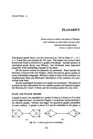
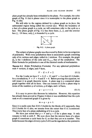
![difference of the faces of G contained in Z. Since the exterior face is thus the
sum (mod 2) of all the interior faces (regarded as edge sets), we see that
m = F — 1. Hencem — q — p + 1 b e c o m e s F - l = £ - F - f l .
Euler’s equation has many consequences.
Corollary 11.1(a) If G is a (p, q) plane map in which every face is an n-cycle,
then
q ~ n(P ~ 2)/(n —2). (11.2)
Proof. Since every face of G is an n-cycle, each line of G is on two faces and
each face has n edges. Thus nr — 2q, which when substituted into (11.1')
gives the result.
A maximal planar graph is one to which no line can be added without
losing planarity. Substituting n — 3 and 4 into (11.2) gives us the next
result.
Corollary 11.1(b) If G is a (p, q) maximal plane graph, then every face is a
triangle and q = 3p — 6. If G is a plane graph in which every face is a 4-cycle,
then q = 2p —4.
Because the maximum number of edges in a plane graph occurs when
each face is a triangle, we obtain a necessary condition for planarity of a
graph in terms of the number of lines.
Corollary 11.1(c) If G is any planar (p, q) graph with p > 3, then q < 3p — 6.
Furthermore, if G has no triangles, then q < 2p — 4.
Corollary 11.1(d) The graphs K s and K 33 are nonplanar.
Proof. The (5, 10) graph K 5 is nonplanar because q = 10 > 9 = 3p — 6;
for K 3 3, q = 9 and 2p — 4 = 8.
As we will soon see, the graphs K s and K 3t3 play a prominent role in
characterizing planarity. The above corollaries are extremely useful in
investigating planar graphs, especially maximal planar graphs.
Corollary 11.1(e) Every planar graph G with p > 4 has at least four points
of degree not exceeding 5.
Clearly, a graph is planar if and only if each of its components is planar.
Whitney [W12] showed that in studying planarity, it is sufficient to consider
2-connected graphs.
Theorem 11.2 A graph is planar if and only if each of its blocks is planar.
It is intuitively obvious that any planar graph can be embedded in the
sphere, and conversely. This fact enables us to embed a planar graph in the
plane in many different ways.
104 PLANARITY](https://image.slidesharecdn.com/graphtheory-181103155731/85/Graph-theory-115-320.jpg)
![PLANE AND PLANAR GRAPHS 105
Theorem 11.3 Every 2-connected plane graph can be embedded in the plane
so that any specified face is the exterior.
Proof. L et/be a nonexterior face of a plane block G. Embed G on a sphere
and call some point interior to/ the “North Pole ” Consider a plane tangent
to the sphere at the South Pole and project* G onto that plane from the
North Pole. The result is a plane graph isomorphic to G in which / is the
exterior face.
Corollary 11.3(a) Every planar graph can be embedded in the plane so that a
prescribed line is an edge of the exterior region.
Whitney also proved that every maximal planar graph is a block,
and more.
Theorem 11.4 Every maximal planar graph with p > 4 points is 3-connected.
Fig. 11.3. Plane wheels.
There are five ways of embedding the 3-connected wheel W5 in the
plane: one looks like Fig. 11.3(a), and the other four look like Fig. 11.3(b).
However, there is only one way of embedding W5on a sphere, an observation
which holds for all 3-connected graphs (Whitney [W 11]).
Theorem 11.5 Every 3-connected planar graph is uniquely embeddable on
the sphere.
Fig. 11.4. Two plane embeddings of a 2-connected graph.
To show the necessity of 3-connectedness, consider the isomorphic
graphs Gj and G2 of connectivity 2 shown in Fig. 11.4. The graph Gl is
embedded on the sphere so that none of its regions are bounded by five
edges while G2 has two regions bounded by five edges.
* This is usually called stereographic projection.](https://image.slidesharecdn.com/graphtheory-181103155731/85/Graph-theory-116-320.jpg)
![106 PLANARITY
A polyhedron is convex if the straight line segment joining any two of its
points lies entirely within it. The next theorem is due to Steinitz and
Rademacher [SR2].
Theorem 11.6 A graph is the 1-skeleton ofa convex 3-dimensional polyhedron
if and only if it is planar and 3-connected.
One of the most fascinating areas of study in the theory of planar
graphs is the interplay between considering a graph as a combinatorial
object and as a geometric figure. Very often the question arises of placing
geometric constraints on a graph. For example, Wagner [W l], Fary [FI],
and Stein [SI5] independently showed that every planar graph can be
embedded in the plane with straight edges.
Theorem 11.7 Every planar graph is isomorphic with a plane graph in which
all edges are straight line segments.
OUTERPLANAR GRAPHS
A planar graph is outerplanar if it can be embedded in the plane so that all its
vertices lie on the same face; we usually choose this face to be the exterior.
Figure 11.5 shows an outerplanar graph (a) and two outerplane embeddings
(b) and (c). In (c) all vertices lie on the exterior face.
(a) (b) (c)
Fig. 11.5. An outerplanar graph and two outerplane embeddings.
In this section we develop theorems for outerplanar graphs parallel
with those for planar graphs. The analogue of Theorem 11.2 is immediate.
Theorem 11.8 A graph G is outerplanar if and only if each of its blocks is
outerplanar.
An outerplanar graph G is maximal outerplanar if no line can be added
without losing outerplanarity. Clearly, every maximal outerplane graph is
a triangulation of a polygon, while every maximal plane graph is a tri
angulation of the sphere. The three maximal outerplane graphs with 6
vertices are shown in Fig. 11.6.
Theorem 11.9 Let G be a maximal outerplane graph with p > 3 vertices all
lying on the exterior face. Then G has p — 2 interior faces.](https://image.slidesharecdn.com/graphtheory-181103155731/85/Graph-theory-117-320.jpg)
![OUTERPLANAR GRAPHS 107
Proof. Obviously the result holds for p = 3. Suppose it is true for p — n
and let G have p = n + 1 vertices and m interior faces. Clearly G must have
a vertex v of degree 2 on its exterior face. In forming G — v we reduce the
number of interior faces by 1 so that m — 1 = n —2. Thus m = n — 1 —
p — 2, the number of interior faces of G.
This theorem has several consequences.
Corollary 11.9(a) Every maximal outerplanar graph G with p points has
a) 2p — 3 lines,
b) at least three points of degree not exceeding 3,
c) at least two points of degree 2,
d) k(G) = 2.
All plane embeddings of K 4 and K l z are of the forms shown in Fig. 11.7,
in which each has a vertex inside the exterior cycle. Therefore, neither of these
graphs is outerplanar. We now observe that these are the two basic non-
outerplanar graphs, following [CH3].
Two graphs are homeomorphic if both can be obtained from the same
graph by a sequence of subdivisions of lines. For example, any two cycles
are homeomorphic, and Fig. 11.8 shows a homeomorph of K 4.
Theorem 11.10 A graph is outerplanar if and only if it has no subgraph
homeomorphic to K 4 or K 2,3 except K4 - x.
It is often important to investigate the complement of a graph wkh a
given property. For planar graphs, the following theorem due to Battle,
(b) (c)
Fig. 11.6. Three maximal outerplanar graphs.
Fig. 11.7. The forbidden graphs for outerplanarity.](https://image.slidesharecdn.com/graphtheory-181103155731/85/Graph-theory-118-320.jpg)
![108 PLANARITY
Harary, and Kodama [BHK1] and proved less clumsily by Tutte [T16],
provides a sufficient condition for the complement of a planar graph to be
planar.
Theorem l l .l l Ever) planar graph with at least nine points has a nonplanar
complement, and nine is the smallest such number.
This result was proved by exhaustion; no elegant or even reasonable
proof is known.
The analogous observation for outerplanar graphs was made in [G5].
Theorem 11.12 Every outerplanar graph with at least seven points has a
nonouterplanar complement, and seven is the smallest such number.
Fig. 11.9. The four maximal outerplanar graphs with seven points.
Proof. To prove the first part, it is sufficient to verify that the complement
of every maximal outerplanar graph with seven points is not outerplanar.
This holds because there are exactly four maximal outerplanar graphs with
p = 7 (Fig. 11.9) and the complement of each is readily seen to be non
outerplanar. The minimality follows from the fact that the (maximal)
outerplanar graph of Fig. 11.6(b) with six points has an outerplanar
complement.
KURATOWSKI’S THEOREM
Until Kuratowski’s paper appeared [K14], it was a tantalizing unsolved
problem to characterize planar graphs. The following proof of his theorem
is based on that by Dirac and Schuster [DS1].](https://image.slidesharecdn.com/graphtheory-181103155731/85/Graph-theory-119-320.jpg)
![kuratow ski’s theorem 109
Theorem 11.13 A graph is planar if and only if it has no subgraph homeo-
morphic to K s or K 33.
Proof. Since K s and K 33 are nonplanar by Corollary 11.1(d), it follows that
if a graph contains a subgraph homeomorphic to either of these, it is also
nonplanar.
The proofofthe converse is a bit more involved. Assume it is false. Then
there is a nonplanar graph with no subgraph homeomorphic to either K 5
or K 33. Let G be any such graph having the minimum number oflines. Then
G must be a block with S{G) > 3. Let x 0 = u0v0 be an arbitrary line of G.
The graph F = G —x 0 is necessarily planar.
We will find it convenient to use two lemmas in the development of the
proof.
Lemma 11.13(a) There is a cycle in F containing u0 and v0.
Proof of Lemma. Assume that there is no cycle in F containing u0 and t?0.
Then u0 and v0 lie in different blocks of F by Theorem 3.3. Hence, there
exists a cutpoint w of F lying on every u0~v0 path. We form the graph F0
by adding to F the lines wu0 and wv0 if they are not already present in F.
In the graph F& u0 and v0 still lie in different blocks, say B l and B2, which
necessarily have the point w in common. Certainly, each of Bx and B2 has
fewer lines than G, so either B l is planar or it contains a subgraph homeo
morphic to K 5or K 33. If, however, the insertion of wu0produces a subgraph
H of Bi homeomorphic to K s or K 3 3, then the subgraph of G obtained bf
replacing wu0 by a path from uQto w which begins with x 0 is necessarily
homeomorphic to H and so to K s or JC3t3, but this is a contradiction. Hence,
Bi and similarly B2 is planar. According to Corollary 11.3(a), both Bx and
B2can be drawn in the plane so that the lines wu0and wv0bound the exterior
region. Hence it is possible to embed the graph F0 in the plane with both
wu0 and wv0 on the exterior region. Inserting x 0 cannot then destroy the
planarity of F0. Since G is a subgraph of F0 -f x 0, G is planar; this contra
diction shows that there is a cycle in F containing u0 and v0.
Let F be embedded in the plane in such a way that a cycle Z containing
u0 and v0 has a maximum number of regions interior to it. Orient the edges
of Z in a cyclic fashion, and let Z[u, v] denote the oriented path from u to v
along Z. If v does not immediately follow u on Z, we also write Z(u, v) to
indicate the subpath of Z[u, v] obtained by removing u and v.
By the exterior of cycle Z,we mean the subgraph of F induced by the
vertices lying outside Z, and the components of this subgraph are called the
exterior components of Z. By an outer piece of Z, we mean a connected sub
graph of F induced by all edges incident with at least one vertex,in some
exterior component or by an edge (if any) exterior to Z meeting two ver
tices of Z. In a like manner, we define the interior of cycle Z, interior com
ponent, and inner piece.](https://image.slidesharecdn.com/graphtheory-181103155731/85/Graph-theory-120-320.jpg)
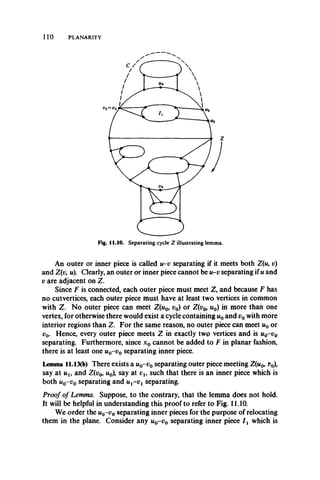
![KURATOWSKfS THEOREM 1 11
Fig. 11.11. The possibilities for nonplanar subgraphs.
nearest to u0in the sense of encountering points of this inner piece on moving
along Z from u0. Continuing out from w0, we can index the u0-v 0 separating
inner pieces 12,1 3, and so on.
Let u2 and u3 be the first and last points of I x meeting Z(u0, v0) and v2
and v3be the first and last vertices of I x meeting Z(v0, u0). Every outer piece
necessarily has both its common vertices with Z on either Z[t>3, u2~ or
Z[u3, p2]> for otherwise there would exist an outer piece meeting Z(u0, v0)
at ux and Z(i?0, u0) at vx and an inner piece which is both u0-v0 separating
and u1- v 1 separating, contrary to the supposition that the lemma is false.
Therefore, a curve C joining v3and u2 can be drawn in the exterior region so
that it meets no edge of F. (See Fig. 11.10.) Thus, I j can be transferred outside
of C in a planar manner. Similarly, the remaining u0-v 0 separating inner
pieces can be transferred outside of Z, in order, so that the resulting graph
is plane. However, the edge x0 can then be added without destroying the
planarity of F, but this is a contradiction, completing the lemma.
Proof of Theorem. Let H be the inner piece guaranteed by Lemma 11.13(b)
which is both u0-v 0 separating and u1~vl separating. In addition, let
w0, Wo, wl5 and w be vertices at which H meets Z(u0, v0 Z(p0, w0), Z(wl5
and Z(vu mx), respectively. There are now four cases to consider, depending
on the relative position on Z of these four vertices.
CASE 1. One of the vertices Wj and w is on Z(m0, v 0 ) and the other is on
Z(v09 u0). We can then take, say, w0 = wx and w'0 = w, in which case G](https://image.slidesharecdn.com/graphtheory-181103155731/85/Graph-theory-122-320.jpg)
![112 PLANARITY
contains a subgraph homeomorphic to K 33, as indicated in Fig. 11.11(a), in
which the two sets of vertices are indicated by open and closed dots.
CASE 2. Both vertices wxand Wxare on either Z(u^ v0) or Z(vq, u0). Without
loss of generality we assume the first situation. There are two possibilities:
either vx # w'0 or vx = W0. If vx # wj>, then G contains a subgraph homeo
morphic to K 33, as shown in Fig. 11.11(b) or (c), depending on whether W0
lies on Z(ux,v x) or Z(vl9 ux respectively. If vx = w'0 (see Fig. 11.1 Id),
then H contains a vertex r from which there exist disjoint paths to wl9 w'l9
and vl9 all of whose vertices (except wi9 w'l9and vx) belong to H. In this case
also, G contains a subgraph homeomorphic to K 3 3.
CASE 3. wx = v0 and Wx # u0. Without loss of generality, let Wx be on
Z(uo, v0). Once again G contains a subgraph homeomorphic to K 33. If
w'0 is on (V& vt then G has a subgraph K 3t3 as shown in Fig. 11.11(e). I£ on
the other hand, w'0 is on Z(vl9 u0%there is a X 3 3 as indicated in Fig. 11.11(f).
This figure is easily modified to show G contains K 3 3 if w'0 = vt.
CASE 4. wx = v0 and w = ti0. Here we assume w0 = ut and w'Q = vu for
otherwise we are in a situation covered by one of the first 3 cases. We
distinguish between two subcases. Let P0 be a shortest path in H from u0
to Vq, and let Px be such a path from ux to vx. The paths P0 and P x must
intersect. If P0 and P x have more than one vertex in common, then G
contains a subgraph homeomorphic to K 3 39 as shown in Fig. 11.11(g);
otherwise, G contains a subgraph homeomorphic to K 5 as in Fig. 11.11(h).
Since these are all the possible cases, the theorem has been proved.
In his paper “How to draw a graph,” Tutte [T17] gives an algorithm
for drawing in the plane as much of a given graph as possible and shows
that whenever this process stops short of the entire graph, it must contain
a subgraph homeomorphic to K s or X 3 3. Thus his algorithm furnishes an
independent proof of Theorem 11.13.
An elementary contraction of a graph G is obtained by identifying two
adjacent points u and vythat is, by the removal of u and v and the addition
Fig. 11.12. Nonplanarity of the Petersen graph.](https://image.slidesharecdn.com/graphtheory-181103155731/85/Graph-theory-123-320.jpg)
![OTHER CHARACTERIZATIONS OF PLANAR GRAPHS 113
of a new point w adjacent to those points to which u or v was adjacent.
A graph G is contractible to a graph H U H can be obtained from G by a
sequence of elementary contractions. For example, as indicated in Fig.
11.12(a) and (b), the Petersen graph is contractible to K 5 by contracting
each of the five lines joining the pentagon with the pentagram to a new
point w,. A dual form of Kuratowski’s theorem (in the sense of duality in
matroid theory) was found independently by Wagner [W2] and Harary
and Tutte [HT3].
Theorem 11.14 A graph is planar if and only if it does not have a subgraph
contractible to K s or K 3 3.
We have just seen that the Petersen graph is contractible to K s. Since
every point has degree 3, it clearly does not have a subgraph homeomorphic
to K s ; Fig. 11.12(c) shows one homeomorphic to K 3 3.
OTHER CHARACTERIZATIONS OF PLANAR GRAPHS
Several other criteria for planarity have been discovered since the original
work of Kuratowski. We have already noted the “dual form” in terms of
contraction in Theorem 11.14. Tutte’s algorithm for drawing a graph in
the plane may also be regarded as a characterization.
Whitney [W12, W14] expressed planarity in terms of the existence of
dual graphs. Given a plane graph G, its geometric dual G* is constructed
as follows: place a vertex in each region of G (including the exterior region)
and, if two regions have an edge x in common, join the corresponding
vertices by an edge x* crossing only x. The result is always a plane pseudo
graph, as indicated in Fig. 11.13 where G has solid edges and its dual G*
dashed edges. Clearly G* has a loop if and only if G has a bridge, and G*
has multiple edges if and only if two regions of G have at least two edges in
common. Thus, a 2-connected plane graph always has a graph or multi
graph as its dual, while the dual of a 3-connected graph is always a graph.
Other examples of geometric duals are given by the Platonic graphs: the
tetrahedron is self-dual, whereas the cube and octahedron are duals, as are
the dodecahedron and the icosahedron.
Fig. 11.13. A plane graph and its geometric dual.](https://image.slidesharecdn.com/graphtheory-181103155731/85/Graph-theory-124-320.jpg)
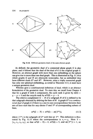
![OTHER CHARACTERIZATIONS OF PLANAR GRAPHS 115
Fig. 11.15. Combinatorial duals.
the defining equation is satisfied. It is of course very difficult to check
whether two graphs are duals using (11.3) since it involves verifying this
equation for every set Y of lines in G.
As with geometric duals, combinatorial duals of planar graphs are not
necessarily unique. However, if two graphs are combinatorial duals of
isomorphic graphs, there is a one-to-one correspondence between their sets
of lines which preserves cycles as sets of lines (that is, their cycle matroids
are isomorphic). The correspondence x, «-►}>, of G* and H* in Fig. 11.14
illustrates this.
Whitney proved that combinatorial duals are equivalent to geometric
duals, giving another criterion for planarity.
Theorem 11.15 A graph is planar if and only if it has a combinatorial dual.
Another criterion for planarity due to MacLane [M l] is expressed in
terms of cyclic structure.
Theorem 11.16 A graph G is planar if and only if every block of G with at least
three points has a cycle basis Z u Z2, • • •, Zmand one additional cycle Z0
such that every line occurs in exactly two of these m + 1 cycles.
We only indicate the necessity, which is much easier. As mentioned
in the proof of Theorem 11.1, all the interior faces of a 2-connected
plane graph G constitute a cycle basis Z 1?Z 2, • • •, Zm, where m is the cycle
rank of G. Let Z0 be the exterior cycle of G. Then obviously each edge of
G lies on exactly two of the m -f 1 cycles Z,.
To prove the sufficiency, it is necessary to construct a plane embedding
of a given graph G with the stipulated properties.](https://image.slidesharecdn.com/graphtheory-181103155731/85/Graph-theory-126-320.jpg)
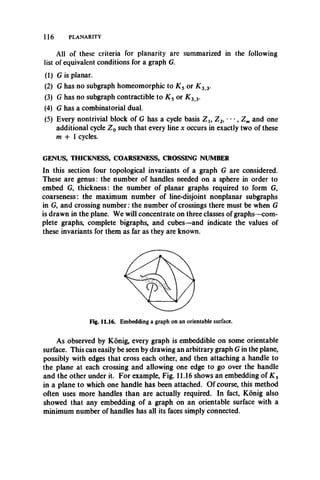
![GENUS, THICKNESS, COARSENESS, CROSSING NUMBER 117
«I «2 u3 UA
3
2
6 4 6 K, «2 U3
Fig. 11.17. An embedding of Kn on the
torus.
Fig. 11.18. A toroidal embedding of
* 4.4-
We have already noted that planar graphs can be embedded on a sphere.
A toroidalgraph can be embedded on a torus. Both K 5and K 33 are toroidal;
in fact Figs. 11.17 and 11.18 show embeddings of X 7 and K+A on the torus,
represented as the familiar rectangle in which both pairs of opposite sides
are identified. No characterization of toroidal graphs analogous to Kura
towski’s Theorem has been found. However, VoUmerhaus [V6] settled a
conjecture of Erdos in the affirmative by proving that for the torus as well
as any other orientable surface, there is a finite collection of forbidden
subgraphs.
The genus y(G) of a graph G is the minimum number of handles which
must be added to a sphere so that G can be embedded on the resulting surface.
Ofcourse, y(G) = 0 ifand only ifG is planar, and homeomorphic graphs have
the same genus.
The first theorem of this chapter presented the Euler characteristic
equation, V — E + F = 2, for spherical polyhedra. More generally, the
genus of a polyhedron* is the number of handles needed on the sphere for
a surface to contain the polyhedron. Theorem 11.1 has been generalized
to polyhedra of arbitrary genus, in a result also due to Euler. A proof may
be found in Courant and Robbins [CR1].
Theorem 11.17 For a polyhedron of genus y with V vertices, E edges and
F faces,
This equation is particularly useful in proving the easy half of the results
to follow on the genus and thickness of particular graphs. Its corollaries,
which offer no difficulty, are often more convenient for this purpose.
* For a combinatorial treatment of the theory of polyhedra, see Grunbaum[GI((|.
V - E + F = 2 - 2 y . (11.4)](https://image.slidesharecdn.com/graphtheory-181103155731/85/Graph-theory-128-320.jpg)
![118 PLANARITY
Corollary 11.17(a) If G is a connected graph of genus y in which every face
is a triangle, then
q = 3(p - 2 + 2y); (11.5)
when every face is a quadrilateral,
q = 2(p - 2 4- 2y). (11.6)
As mentioned in [BH2], it is easily verified from these two equations
that the genus of a graph has the following lower bounds.
Corollary 11.17(b) If G is a connected graph of genus y, then
y > h - % p - 2); (11.7)
if G has no triangles, then
y > h - ¥ p - 2). (ii.8)
The determination of the genus of the complete graphs has been a long,
interesting, difficult, successful struggle. In its dual form, it was known as
the Heawood Conjecture and stood unproved from 1890 to 1967. We
return to this aspect of the problem in the next chapter. There have been
many contributors to this result and the coup de grace, settling the conjecture
in full, was administered by Ringel and Youngs [RY1].
Theorem 11.18 For p > 3, the genus of the complete graph is
The proof of the easier half of equation (11.9) is due to Heawood [H38].
It amounts to substituting q(Kp) into inequality (11.7) to obtain
_ ' / n ( i> - 3 X p - 4 )
* i ? ) - i '" ~ 21 n •
Then since the genus of every graph is an integer,
The proof that this expression is also an upper bound for y{Kp) can only be
accomplished by displaying an embedding of K p into an orientable surface
of the indicated genus. When Heawood originally stated the conjecture
in 1890, he proved that y(K7) = 1, as verified by the embedding shown in
Fig. 11.17, which triangulates the torus.
Heffter proved (11.9) in 1891 for p = 8 through 12. Not until 1952 did
Ringel prove it for p = 13. At that stage, it was realized that because of its
form, it was natural to try to settle the question for one residue class of p](https://image.slidesharecdn.com/graphtheory-181103155731/85/Graph-theory-129-320.jpg)
![GENUS, THICKNESS, COARSENESS, CROSSING NUMBER 119
modulo 12 at a time. Writing p = 12s + r, Ringel (see [RIO]) proved (11.9)
in 1954 for all complete graphs K p with r = 5. During 1961-65, Ringel
extended the result to r = 7, 10, and 3, and concurrently Youngs [Y l] with
his colleagues Gustin, Terry, and Welch settled the cases r = 4, 0, 1, 9, 6. In
1967-68, Ringel and Youngs [RY1, 2] worked together to achieve appro
priate embeddings of K p for r = 2, 8, and 11. The isolated cases p = 18,
20, and 23 remained unproved by these methods. The proof was completed
by the Professor of French Literature at the University of Montpellier,
named Jean Mayer, when he embedded K p for these three values of p,
see [M6].
For complete bigraphs, the corresponding result is less involved, and
was obtained by Ringel alone. Since inequality (11.8) applies to the graph
Km,n we have
, v , ^ 1 1 , , (m - 2)(n - 2)
y(Km.„) > -^mn - ~(m + n - 2) = ----------- - ------------ .
The other inequality is demonstrated [R12] by displaying a suitable em
bedding of Kmn.
Theorem 11.19 The genus of the complete bigraph is
**..■> - ~ 24X" ~ 2>}. (11.10)
The genus of the cube was derived by Ringel [R13] and Beineke and
Harary [BH3]. For the graph Qn, we have p = 2" and q = «2n-1, so that
by (11.8),
y(Qn) > 1 -f (n - 4)2n_3,
proving the easier half of the next equation.
Theorem 11.20 The genus of the cube is
?(C„) = 1 + (n - 4)2"“ 3. (11.11)
We now mention some more general considerations involving genus.
It was shown in Battle, Harary, Kodama and Youngs [BHKY1] that the
genus of a graph depends only on the genus of its blocks, as anticipated in
Theorem 11.2.
Theorem 11.21 If a graph G has blocks Blt B2, • • •, B„, then
y(G) = £ y(B,). (11.12)
This result was generalized slightly by Harary and Kodama [HK1].
Recall from Theorem 5.8 that two (n + 1^components of a graph have at
most n points in common.](https://image.slidesharecdn.com/graphtheory-181103155731/85/Graph-theory-130-320.jpg)
![120 PLANARITY
Theorem 11.22 Let an w-connected graph G be the union of two (n + 1)-
components B and C. Let vl9 • • •, vn be the set of points of B n C. Call G0
the graph obtained by adding line t)tVj to G. If y(G0) = y(G) + 1 whenever
1 < i < j < n, then
y(G) = y(£) + y(C) 4- n - 1. (11.13)
We have already observed in Theorem 11.11 that every planar graph
with 9 points has a nonplanar complement. Define the thickness 6{G) of a
graph as the minimum number of planar subgraphs whose union is G.
Then Theorem 11.11 can be stated in the form 0(Kg) > 2. Actually the thick
ness of K 9is 3 but K 9is critical with respect to thickness since 0(K9 — x) = 2.
Therefore 0{Kp) = 2 for p = 5 to 8. Of course 0(G) = 1 if and only if G
is planar. Since a maximal planar graph has q = 3p - 6 lines, it follows
that the thickness 0 of any (p, q) graph has the bound,
7 = 6 - < " 14>
This observation is useful in making conjectures about thickness and proving
the easier half.
The thickness of the complete graphs was investigated in [BH5] and
Beineke [B6], Applying (11.14) to we find
w n > - D/2
* -jjp - 2 ) ■
Applying some algebraic manipulations, we obtain
Theorem 11.23 Whenever p ^ 4 (mod 6), the thickness of the complete graph
m P) = (n.15)
unless p — 9.
When p = 4 (mod 6), sometimes equation (11.15) holds and sometimes
it doesn’t. For 0(K1O) = 3 # [^ ], but Hobbs and Grossman [HG1]
produced a decomposition of K 22 into 4 = [” ] planar subgraphs and
Beineke [B6] showed that 6(K2a) = 5 = [^ ]. Very recently, Jean Mayer
(again!) obtained constructions showing that 0{K3A) = 6 and 0(KM) = 7.
The onlyvalueof p < 45for which 6(Kp) is notyet known is p = 16. It is
conjecturedthat0(K16) = 4, but for all p = 4 (mod 6), and p > 46, that
(11.15) holds.
The thickness of complete bigraphs was studied in [BHM1] and Beineke
[B7],](https://image.slidesharecdn.com/graphtheory-181103155731/85/Graph-theory-131-320.jpg)
![GENUS, THICKNESS, COARSENESS, CROSSING NUMBER 121
Theorem 11.24 The thickness of the complete bigraph is
2(m + n — 2)
mn
}
(11.16)
except possibly when m < n, mn is odd, and there exists an integer k such
that n = [2k(m — 2)/(m — 2k)].
Corollary 11.24(a) The thickness of Knn is [(n -f 5)/4].
The corresponding problem for the cube was settled byKleinert [K8].
Theorem 11.25 The thickness of the cube is
P. Erdos (verbal communication) made a fortuitous slip, while trying
to describe the concept of thickness. By speaking of the maximum number
of line-disjoint nonplanar subgraphs contained in the given graph G, he
first defined the coarseness £(G). Thus both thickness and coarseness involve
constructions which factor a graph into spanning subgraphs (planar and
nonplanar respectively) in the sense of Chapter 9. Formulas for the coarse
ness of a complete graph are not as neat as those for other topological
invariants. The reason is that K z 3 or a homeomorph thereof is a most
convenient subgraph for coarseness constructions. This suggests the reason
for the form of the next result due to Guy and Beineke [GB1]. Figure 11.19
shows four line-disjoint homeomorphs of K 3 3 contained in K l0.
Theorem 11.26 The coarseness of the complete graphs is given by
All of the values of £(Kp)are either known exactly from (11.18) or have the
value given in Table 11.1 or 1 greater; see [GB1].
For the coarseness of the complete bigraph, the results of Beineke and
Guy [BG1] are incomplete and involve many cases.
(11.17)
t(K 3n) =
(p = 3n > 30),
(11.18)
(p = 3n + 1 > 19
and p ^ 9r + 7),](https://image.slidesharecdn.com/graphtheory-181103155731/85/Graph-theory-132-320.jpg)
![122 PLANARITY
Fig. 11.19. Four nonplanar subgraphs of Kl0.
Theorem 11.27 The coarseness of the complete bigraph K mnsatisfies
i(K 3r+i,3s+e) = rs + min ^ y j , j^ y j^
[fl
£(K3r+2,3S) = rS +
< rs 4 min
e(K3r+2f3s+i) <
for d = 0 or 1 and e = 0 or 1.
when r > 1.
8r 4- 16s 4 2. ( r 4 si I"2s! TSr 4 16s 4 2~1
— 55— J J
( M - « )
Z(K3r+2,3 s + :
> rs 4 max
(These are equal when r > 2s.)
< rs 4 mm
(11.19)
for r > 2, s > 7.
> rs 4
The crossing number v(G) of a graph G is the minimum number of
pairwise intersections of its edges when G is drawn in the plane. Obviously
v(G) = 0 if and only if G is planar. The exact value of the crossing number
has not yet been determined for any of the three families of graphs; only
upper bounds are definitely established. The prevailing conjecture is that
the bounds in (11.20) and (11.21) are exact. Several authors have deluded
themselves into thinking they had proved equality. For details, see Guy
[G12],](https://image.slidesharecdn.com/graphtheory-181103155731/85/Graph-theory-133-320.jpg)
![EXERCISES 123
Table 11.1
CONJECTURED VALUES FOR Z(Kp)
p 13 18 21 24 27 9n + 7
7 15 21 28 36 (9n2 + 13n + 2)12
Theorem 11.28 The crossing number of the complete graph satisfies the
inequality
Theorem 11.29 The crossing number of the complete bigraph satisfies the
inequality
m m — 1" n
2_ 2 2J
(11.21)
T. Saaty showed that (11.20) is an equation for p < 10 while D. Kleitman
proved equality in (11.21) for m < 6. These are the only known values of
v(Kp) and v(Kmn). For the cubes, no one has even conjectured what is v.
EXERCISES
11.1 If a (plt qi) graph and a (p2, q2) graph are homeomorphic, then
Pi + = Pi + <?i*
11.2 Every plane eulerian graph contains an eulerian trail that never crosses itself.
11.3 A 3-connected graph with p > 6 is planar if and only if no subgraph is homeo
morphic to K3t3. (D. W. Hall [H6])
*11.4 Every 4-connected planar graph is hamiltonian. (Tutte [T11|])
11.5 Every 5-connected planar graph has at least 12 points. Construct one.
11.6 There is no 6-connected planar graph.
*11.7 If Gis a maximal plane graph in which every triangle bounds a region, then Gis
hamiltonian. (Whitney, Ann. Math., 32 (1931), 378-390.)
11.8 Not every maximal planar graph is hamiltonian. (Whitney, same as above.)
11.9 If, in a drawing of G in the plane, every pair of nonadjacent edges cross an even
number of times, then G is planar.
(R. L. Brooks, C. A. B. Smith, A. H. Stone, and W. T. Tutte)
11.10 Prove or disprove: every connected nonplanar graph has K5 or K33 as a
contraction.](https://image.slidesharecdn.com/graphtheory-181103155731/85/Graph-theory-134-320.jpg)
![124 PLANARITY
11.11 Prove or disprove:A graph is planar if and only if every subgraph with at most
six points of degree at least 3 is homeomorphic to a subgraph of K2 4 PA.
11.12 Prove or disprove: The cycle basis of a plane graph consisting of the interior
faces always comes from a tree (cf. Chapter 4).
*11.13 Every triply connected planar graph has a spanning tree with maximum degree 3.
(Barnette [B3])
11.14 A plane graph is 2-connected if and only if its geometric dual is 2-connected.
11.15 All wheels are self-dual.
11.16 The square of a connected graph Gis outerplanar ifand only if G is K3or a path.
11.17 The following statements are equivalent:
(1) The line graph L(G) is outerplanar.
(2) The maximum degree A(G) < 3 and every point of degree 3 is a cutpoint.
(3) The total graph T(G) is planar.
(Chartrand, Geller, and Hedetniemi [CGH2], Behzad [B4])
11.18 A graph G other than <D> has a planar square ifand only ifA(G) < 3, every point
of degree 3 is a cutpoint, and all blocks of G with more than 3 points are even cycles.
(Harary, Karp, and Tutte [HKT1])
11.19 A graph G has a planar line graph if and only if G is planar, A(G) < 4, and every
point of degree 4 is a cutpoint. (Sedlacek [S10])
11.20 Find the genus and crossing number of the Petersen graph.
11.21 Prove or disprove: A nonplanar graph G has v = 1 if and only if G — x is
planar for some line x.
11.22 The arboricity of every planar graph is at most 3. Construct a planar graph with
arboricity 3.
11.23 Every graph is homeomorphic to a graph with arboricity 1 or 2, and hence of
thickness 1 or 2.
11.24 The skewness of G is the minimum number of lineswhose removal results in a
planar graph. Find the skewness of
a)K„, b) Km<n, c) g„. (A. Kotzig)
11.25 If G is outerplanar without triangles, then
q < OP - 4)/2.
11.26 If G is a graph such that for any two points, there are at most two point-disjoint
paths of length greater than 1joining them, then
a) G is planar.
b) q < 2p —2.
c) If G is nonseparable and p > 5, then there is a unique hamiltonian cycle.
(Tang [T2])
11.27 Embed the cube Qx on the surface of a torus.](https://image.slidesharecdn.com/graphtheory-181103155731/85/Graph-theory-135-320.jpg)
![EXERCISES 125
11.28 The genus y of any graph G with girth g has the lower bound
*11.29 y(Kt - ( n ~n,n,n) ( ^ J '
(Beineke and Harary [BH2])
(G. Ringel)
11.30 If Gxand G2are homeomorphic, then £(GX) = £(G2) and vfGJ = v(G2).
11.31 The maximum number of line-disjoint K3>3 subgraphs in Kmnis
Thus for all n,
. ( Y m Y Y n T
I)
(Beineke and Guy [BG1])](https://image.slidesharecdn.com/graphtheory-181103155731/85/Graph-theory-136-320.jpg)
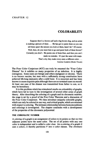
![THE CHROMATIC NUMBER 127
1«---------- *2 2 ----------*3 2 ----------- 3
1 1------------>2 lo----------- »4
l i ----------i 2 3*---------- *1 3*----------- *2
(a) (b) (c)
Fig. 12.1. T h re e c o lo rin g s o f a g ra p h .
number x(G) is defined as the minimum n for which G has an n-coloring.
A graph G is n-colorable if x(G) < n and is n-chromatic if x(G) = n.
Since G obviously has a p-coloring and a ^(G)-coloring, it must also
have an n-coloring whenever x(G) < n < p. The graph of Fig. 12.1 is
2-chromatic; n-colorings for n = 2, 3, 4 are displayed, with positive integers
designating the colors.
The chromatic numbers of some of the familiar graphs are easily
determined, namely x(Kp) = p, x(Kp - x) = p - 1, x(Kp) = 1, = 2,
X(C2„) = 2, *(C2„+i) = 3, and for any nontrivial tree T, *(T) = 2.
Obviously, a graph is 1-chromatic if and only if it is totally disconnected.
A characterization of bicolorable (2-colorable) graphs was given by Konig
[K10, p. 170], as Theorem 2.4 already indicates.
Theorem 12.1 A graph is bicolorable if and only if it has no odd cycles.
It is likely to remain an unsolved problem to provide a characterization
of n-colorable graphs for n > 3, since such a criterion even for n = 3 would
help to settle the 4CC. No convenient method is known for determining the
chromatic number of an arbitrary graph. However, there are several known
bounds for %(G) in terms of various other invariants. One obvious lower
bound is the number of points in a largest complete subgraph of G. We now
consider upper bounds, the first of which is due to Szekeres and Wilf [SW1].
Theorem 12.2 For any graph G,
X(G) < 1 + max S{G'% (12.1)
where the maximum is taken over all induced subgraphs G of G.
Proof! The result is obvious for totally disconnected graphs. Let Gbe an arbi
trary n-chromatic graph, n > 2. Let H be any smallest induced subgraph such
that x(H) = n. The graph H therefore has the property that x(H - v) = n — 1
for all its points v. It follows that deg v > n — 1 so that 5(H) > n — 1 and
hence
n — I < 5(H) < max 5(H') < max <5(G'),
the first maximum taken over all induced subgraphs H ' of H and the second](https://image.slidesharecdn.com/graphtheory-181103155731/85/Graph-theory-138-320.jpg)
![128 COLORABILITY
over all induced subgraphs G' of G. This implies that
X(G) = n < 1 + max S(G’).
Corollary 12.2(a) For any graph G, the chromatic number is at most one
greater than the maximum degree,
X < 1 + A. (12.2)
Brooks [B16] showed, however, that this bound can often be improved.
Theorem 12.3 If A(G) = n > 2, then G is n-colorable unless
i) n = 2 and G has a component which is an odd cycle, or
ii) n > 2 and K n+x is a component of G.
A lower bound, noted in Berge [B12, p. 37] and Ore [05, p. 225], and
an upper bound, Harary and Hedetniemi [HH1], involve the point inde
pendence number p0 of G.
Theorem 12.4 For any graph G,
p / P o < X < P ~ P o + I- (12.3)
Proof. If x(G) = w, then V can be partitioned into n color classes
Vmeach of which, as noted above, is an independent set of points. If | — ph
then every p{ < p0 so that p = I < nf}0.
To verify ihe upper bound, let S be a maximal independent set containing
P0 points. It is clear that x(G — S) > x(G) — 1. Since G — S has p —po
points, x(G - S) < p - p0. Therefore, x(G) < x(G - S) + 1 < p - p0 + 1.
None of the bourtds presented here is particularly good in the sense
that for any bound and for every positive integer n, there exists a graph G
such that x(G) differs from the bound by more than n.
From the discussion thus far, one may very well be led to believe that
all graphs with large chromatic number have large cliques and hence contain
triangles. In fact, Dirac [D7] asked if there exists a graph with no triangles
but arbitrarily high chromatic number. This was answered affirmatively
and independently by Blanche Descartes* [D3], Mycielski [M l9], and
Zykov [Z l]. Their result was extended by Kelly and Kelly [KK1], who
proved that for all n > 2, there exists an n-chromatic graph whose girth
exceeds 5. In the same paper, they conjectured the following theorem,
which was first proved by Erdos [E2] using a probabilistic argument and
later by Lovasz [L5] constructively.
* This so-called lady is actually a nonempty subset of (Brooks, Smith, Stone, Tutte}; in this
case {Tutte}.](https://image.slidesharecdn.com/graphtheory-181103155731/85/Graph-theory-139-320.jpg)
![THE CHROMATIC NUMBER 129
Theorem 12.5 For every two positive integers m and n, there exists an n-
chromatic graph whose girth exceeds m.
The number x = x(G) = x(G) *s the minimum number of subsets which
partition the point set of G so that each subset induces a complete subgraph
of G. It is clear that x(G) > J30(G). Bounds on the sum and product of the
chromatic numbers of a graph and its complement were developed by
Nordhaus and Gaddum [NG1].
Theorem 12.6 For any graph G, the sum and product of x and x satisfy the
inequalities:
2y/p £ x + X ^ P + I (12.4)
p < xx £ ' ^12'5*
Proof Let G be n-chromatic and let Vl9 V2, • • •, Vnbe the color classes of G,
where |V{ = pf. Then of course I p, = p and max p, > p/n. Since each Vt
induces a complete subgraph of G, x > max pt > p/n so that xx ^ P- Since
the geometric mean of two positive numbers never exceeds their arithmetic
mean, it follows that jf + > 2v/p. This establishes both lower bounds.
To show that x + X ^ P + h we use induction on p, noting that
equality holds when p = 1. We thus asfsume that x(G) + x(G) < p for all
graphs G having p — 1 points. Let H and H be complementary graphs
with p points, and let v be a point of H. Then G = H — v and G = H — v
are complementary graphs with p — 1 points. Let the degree of v in H
be d so that the degree of v in H is p —d — 1. It is obvious that
X(H) < x(G) + 1 and *(tf) < x(G) + 1.
If either
X(H) < x(G) + 1 or x(H) < x(G) + 1,
then x(H) + x(H) < p + 1. Suppose then that x(H) = x(G) + 1 and
X(H) = x(G) + 1. This implies that the removal of v from H, producing G,
decreases the chromatic number so that d > x(G). Similarly
p - d — 1 > x(G);
thus x(G) + x(G) < p — 1. Therefore, we always have
X(H) + x(H) < p + 1.
Finally, applying the inequality 4*x < (x + X)2 we see that
XX < [(P + D /2]2.](https://image.slidesharecdn.com/graphtheory-181103155731/85/Graph-theory-140-320.jpg)
![130 COLORABILITY
THE FIVE COLOR THEOREM
Although it is not known whether all planar graphs are 4-colorable, they
are certainly 5-colorable. In this section we present a proof of this famous
result due to Heawood [H38].
Theorem 12.7 Every planar graph is 5-colorable.
Proof. We proceed by induction on the number p of points. For any planar
graph having p < 5 points, the result follows trivially since the graph is
p-colorable.
As the inductive hypothesis we assume that all planar graphs with p
points, p > 5, are 5-colorable. Let G be a plane graph with p 4- 1 vertices.
By Corollary 11.1(e), G contains a vertex v of degree 5 or less. By hypothesis,
the plane graph G — v is 5-colorable.
Consider an assignment of colors to the vertices of G — v so that a
5-coloring results, where the colors are denoted by ci9 1 < i < 5. Certainly,
if some color, say cj9 is not used in the coloring of the vertices adjacent with
v9then by assigning the color Cj to v, a 5-coloring of G results.
This leaves only the case to consider in which deg v = 5 and five colors
are used for the vertices of G adjacent with v. Permute the colors, ifnecessary,
so that the vertices colored cl9 c2, c3, c4, and c5 are arranged cyclically
about v. Now label the vertex adjacent with i; and colored c, by rf, 1 < i < 5
(see Fig. 12.2).
Let G13 denote the subgraph of G — v induced by those vertices colored
Cj or c3. If vt and v3belong to different components of G13, then a 5-coloring
of G — v may be accomplished by interchanging the colors of the vertices
in the component of G13 containing vv In this 5-coloring, however, no
vertex adjacent with v is colored cl9 so by coloring v with the color cl9 a
5-coloring of G results.
If, on the other hand, and v3 belong to the same component of G13,
then there exists in G a path between vx and v3 all of whose vertices are
colored cx or c3. This path together with the path vxvv3 produces a cycle
which necessarily encloses the vertex v2 or both the vertices and v5. In any
Fig. 12.2. A step in the proof of the Five Color Theorem.](https://image.slidesharecdn.com/graphtheory-181103155731/85/Graph-theory-141-320.jpg)
![THE FOUR COLOR CONJECTURE 131
case, there exists no path joining v2and v4, all of whose vertices are colored c2
or c4. Hence, if we let G24 denote the subgraph of G — v induced by the
vertices colored c2 or c4, then v2 and v4 belong to different components
of G24. Thus if we interchange colors of the vertices in the component of
G24 containing t?2, a 5-coloring of G — t; is produced in which no vertex
adjacent with v is colored c2. We may then obtain a 5-coloring of G by
assigning to v the color c2.
THE FOUR COLOR CONJECTURE
In Chapter 1 we mentioned that the 4CC served as a catalyst for graph
theory through attempts to settle it. We now present a graph-theoretic
discussion of this infamous problem. A coloring of a plane map G is an
assignment of colors to the regions of G so that no two adjacent regions are
assigned the same color. The map G is said to be n-colorable if there is a
coloring of G which uses n or fewer colors. The original conjecture as
described in Chapter 1 asserts that every plane map is 4-colorable.
Four Color Conjecture (4CC) Every planar graph is 4-colorable.
We emphasize that coloring a graph always refers to coloring its vertices
while coloring a map indicates that it is the regions which are colored!
Thus the conjecture that every plane map is 4-colorable is in fact equivalent
to this statement of the Four Color Conjecture. To see this, assume the
4CC holds and let G be any plane map. Let G* be the underlying graph of
the geometric dual of G. Since two regions of G are adjacent if and only
if the corresponding vertices of G* are adjacent, map G is 4-colorable
because graph G* is 4-colorable.
Conversely, assume that every plane map is 4-colorable and let H be
any planar graph. Without loss of generality, we suppose H is a connected
plane graph. Let H* be the dual of H, so drawn that each region of H *
encloses precisely one vertex of H. The connected plane pseudograph H*
can be converted into a plane graph //' by introducing two vertices into each
loop of H* and adding a new vertex into each edge in a set of multiple edges.
The 4-colorability of H' now implies that H is 4-colorable, completing the
verification of the equivalence.
If the 4CC is ever proved, the result will be best possible, for it is easy
to give examples of planar graphs which are 4-chromatic, such as K 4 and
W6(see Fig. 12.3).
Each of the graphs K 4 and W6 has more than 3 triangles, which is
necessary according to a theorem of Grunbaum [G9].
Theorem 12.8 Every planar graph with fewer than 4 triangles is 3-colorable,
From this the following corollary is immediate; it was originally proved
by Grotzsch [G8].](https://image.slidesharecdn.com/graphtheory-181103155731/85/Graph-theory-142-320.jpg)
![132 COLORABILITY
Fig. 12.3. Two 4-chromatic planar graphs.
Corollary 12.8(a) Every planar graph without triangles is 3-colorable.
Any plane map which requires 5 colors will necessarily contain a large
number of regions, for Ore and Stemple [OS1] showed that all plane maps
with up to 39 regions are 4-colorable, increasing by 4 regions the earlier
result of this kind.5,1 All evidence indicates that the Four Color Conjecture
is true. However, attempts to prove the 4CC using the plane map formulation
can be directed at a special class of plane maps, as we shall now see.
Theorem 12.9 The Four Color Conjecture holds if and only if every cubic
bridgeless plane map is 4-colorable.
Proof. We have already seen that every plane map is 4-colorable if and
only if the 4CC holds. This is also equivalent to the statement that every
bridgeless plane map is 4-colorable since the elementary contraction of
identifying the endvertices of a bridge affects neither the number of regions
in the map nor the adjacency of any of the regions.
Certainly, if every bridgeless plane map is 4-colorable, then every cubic
bridgeless plane map is 4-colorable. In order to verify the converse, let G
be a bridgeless plane map and assume all cubic bridgeless plane maps are
4-colorable. Since G is bridgeless, it has no endvertices. If G contains a
vertex v of degree 2 incident with edges y and z, we subdivide y and z, denoting
the subdivision vertices by u and w, respectively. We now remove v, identify u
with one of the vertices ofdegree 2 in a copy of the graph K A — x and identify
w with the other vertex of degree 2 in K+ —x. Observe that each new
vertex added has degree 3 (see Fig. 12.4). If G contains a vertex v0 of degree
n > 4 incident with edges x u x 2, • **, arranged cyclically about v0, we
subdivide each x ( producing a new vertex vt. We then remove v0 and add
the new edges 17^2, v2v3, • • •, vn-iv w vnvx. Again each ofthe vertices so added
has degree 3.
Denote the resulting bridgeless cubic plane map by G', which, by
hypothesis, is 4-colorable. If for each vertex i; of G with deg v ^ 3, we
* Finck and Sachs [FS1] proved that every plane graph with at most 21 triangles is 4-colorable.](https://image.slidesharecdn.com/graphtheory-181103155731/85/Graph-theory-143-320.jpg)
![THE FOUR COLOR CONJECTURE 133
After
*4
Fig. 12.4. Conversion of a graph into a cubic graph.
identify all the newly added vertices associated with v in the formation of
G', we arrive at G once again. Thus let there be given a 4-coloring of G'.
The aforementioned contraction of G' into G induces an m-coloring of G,
m < 4, which completes the proof.
Another interesting equivalence was proved by Whitney [W16].
Theorem 12.10 The Four Color Conjecture holds if and only if every
hamiltonian planar graph is 4-colorable.
As there are equivalents of the Four Color Conjecture involving the
coloring of regions, so too is there an equivalent of the 4CC concerned
with the coloring of lines.
A line-coloring of a graph G is an assignment of colors to its lines so that
no two adjacent lines are assigned the same color. An n-line-coloring of G
is a line-coloring of G which uses exactly n colors. The line-chromatic
number* x'(G) is the minimum n for which G has an n-line-coloring. It follows
that for any graph G which is not totally disconnected, x'(G) = #(L(G)).
Tight bounds on the line-chromatic number were obtained** by Vizing [V4].
Theorem 12.11 For any graph G, the line-chromatic number satisfies the
inequalities:
A < x' < A 4- 1. (12.6)
* Sometimes called the chromatic index.
** A proof in English can be found in Ore [07, p. 248].](https://image.slidesharecdn.com/graphtheory-181103155731/85/Graph-theory-144-320.jpg)
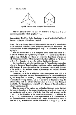
![THE HEAWOOD MAP-COLORING THEOREM 135
other hand, we also have
£ c(v) = ct + c2 + • *• 4- cn + 2{dt -f d2 + *• * 4- dm)
= ct + c2 + • • • -f
since every element of F is self-inverse. Thus cx -f c2 + • *• + cn — k0. It
is now a routine matter to show that this constitutes a 4-coloring of the regions
of G, completing the proof.
Since each line color class resulting from an n-line coloring of a regular
graph G of degree n is a 1-factor of G, the preceding result produces another
equivalent of the Four Color Conjecture.
Corollary 12.12(a) The Four Color Conjecture holds if and only if every
bridgeless, cubic planar graph is 1-factorable.
Theorem 12.12 has been generalized in terms of factorization (see Ore
[07, p. 103]).
Theorem 12.13 A necessary and sufficient condition that a connected planar
map G be 4-colorable is that G be the sum of three subgraphs Gu G2, G3such
that for each point v, the number of lines of each Gf incident with v are all
even or all odd.
Although it is the 4CC which has received the preponderance ofpublicity,
there are several other conjectures dealing with coloring. One of the most
interesting of these involves contractions and is due to Hadwiger [H I].
Hadwiger’s Conjecture. Every connected n-chromatic graph is contractible
to K n.
Not surprisingly, this conjecture is related to the 4CC. Hadwiger’s
Conjecture is known to be true for n < 4, a result of Dirac [D5]. For n — 5,
this conjecture states that every 5-chromatic graph G is contractible to K 5.
By Theorem 11.14, every such graph G is necessarily nonplanar. Thus
Hadwiger’s Conjecture for n = 5 implies the 4CC. The converse was
established by Wagner [W3].
Theorem 12.14 Hadwiger’s Conjecture for n = 5 is equivalent to the Four
Color Conjecture.
THE HEAWOOD MAP-COLORING THEOREM
Let S„ be the orientable surface of genus n ;thus, Snis topologically equivalent
to a sphere with n handles. The chromatic number of Sw denoted x(S„)> *s the
maximum chromatic number among all graphs which can be embedded
on Sn. The surface S0 is simply the sphere and the determination of x(S0)
is the problem we have already encountered on several occasions. The Four](https://image.slidesharecdn.com/graphtheory-181103155731/85/Graph-theory-146-320.jpg)
![136 COLORABILITY
*(S,
Color Conjecture states that x.(S0) = 4 although, of course, we know only
(by Theorem 12.7) that x(S0) is 4 or 5.
For the torus, Heawood [H38] was able to prove that x{St) = 7. The
inequality x ^ ) > 7 follows from the fact that it is possible to embed K 1
on the torus. This is shown in Fig. 11.17. The equality x(Si) = 7 comes from
the fact that Heawood was also able to prove (see the proof of Theorem 12.15
below) that the chromatic number of the orientable surface of positive
genus n has the upper bound
„> < [ W ‘ + 48"] (» > 0). (12.7)
For n — 1, we have x(Si) < 7, so that x(Si) = 7.
Heawood, who found the error in Kempe’s “proof’ of the Four Color
Conjecture, was himself not infallible. He believed that he had proved
equality in his formula, but just one year later, Heffter [H40] pointed out
errors of omission in Heawood’s arguments resulting in only the inequality
(12.7). Heffter did prove equality for 0 < n < 6. Eventually, the statement
that equality holds in Heawood’s formula became known as the Heawood
Map-Coloring Conjecture. We now show that when Ringel and Youngs
proved that y(Kp) = {(p — 3)(p —4)/12}, Theorem 11.18, they settled this
conjecture.
Theorem 12.15 (Heawood Map-Coloring Theorem). For every positive
integer n, the chromatic number of the orientable surface of genus n is
given by
X(S,.) = (« > 0). (12.8)
Proof. We first prove inequality (12.7). Let G be a (p, q) graph embedded
on Sn. We may assume G is a triangulation, since any graph can be aug
mented to a triangulation of the same genus by adding edges, without
reducing x- If d is the average degree of the vertices of G, then p, q, and r (the
number of regions) are related by the equations
dp = 2q = 3r. (12.9)
Solving for q and r in terms of p and using Euler’s equation (11.4), we obtain
d = 12(n - l)/p + 6. (12.10)
Since d < p — 1, this gives the inequality
p - 1 > 12(it - 1)/p + 6. (12.11)
Solving for p and taking the positive root, we obtain
(12.12)](https://image.slidesharecdn.com/graphtheory-181103155731/85/Graph-theory-147-320.jpg)
![UNIQUELY COLORABLE GRAPHS 137
Let H(n) be the right-hand side of (12.8). Then we must show that
H{n) colors are sufficient to color the points of G. Clearly if p - H(n) we
have enough colors. If, on the other hand, p > H(n), we substitute H(n) for
p in (12.10), to obtain the inequality
d < 12(n - 1)/H(n) + 6 = H(n) - 1, (12.13)
with the latter equality obtained by routine algebraic manipulation. Thus
when p > H(n), there is a point v of degree at most H(n) - 2. Identify v
and any adjacent point (by an elementary contraction) to obtain a new
graph G'. If p' = p — 1 = H(n), then G' can be colored in H(n) colors.
If p' > H(n), repeat the argument. Eventually an H(n)-colorable graph will
be obtained. It is then easy to see that the coloring of this graph induces a
coloring of the preceding one in H(n) colors, and so forth, so that G itself
is H(n)-colorable.
The other half of the theorem is the difficult part, but Ringel and Youngs
have provided the means. If the complete graph K p can be embedded in
Sw then by equation (11.9),
* > , ( * , ) - j 1' - ” 1’ - 41}. (12.14,
Setting p to be the largest integer satisfying Eq. (12.14), we have
(p - 3Xp - 4) f(p - 3Xp - 4)] f(p - 2Xp - 3 ) , (p - 2Kp - y3)
— --------12— } * " * { ---------12 J '
Solving for p we find
1 <
12
5 + y T T W t 7 + J l -f 48n
Y__--------- < P <------- --------------
2 - 2
So
1,2.15,
Since x(KP) = we have found a graph with genus n and chromatic
number equal to H(n). This shows that H(n) is a lower bound for x(S„) and
completes the proof. Note: (12.8) specialized to n = 0 is precisely the 4CC.
UNIQUELY COLORABLE GRAPHS
Let G be a labeled graph. Any x(G)-coloring of G induces a partition of the
point set of G into x(G) color classes. If x(G) = n and every n-coloring of G
induces the same partition of V, then G is called uniquely n-colorahle or
simply uniquely colorable. The graph G of Fig. 12.6 is uniquely 3-colorable
since every 3-coloring of G has the partition {uj}, {u2, u4}, {u3, u5} while
the pentagon is not uniquely 3-colorable; indeed, five different partitions
of its point set are possible.](https://image.slidesharecdn.com/graphtheory-181103155731/85/Graph-theory-148-320.jpg)
![138 COLORABILITY
G:
Fig. 12.6. A uniquely colorable graph.
We begin with a few elementary observations concerning uniquely
colorable graphs. First, in any n-coloring of a uniquely n-colorable graph G,
every point v of G is adjacent with at least one point of every color different
from that assigned to v; for otherwise a different n-coloring of G could be
obtained by recoloring v. This further implies that 5(G) > n — 1. A
necessary condition for a graph to be uniquely colorable was found by
Cartwright and Harary [CH2].
Theorem 12.16 In the n-coloring of a uniquely n-colorable graph, the
subgraph induced by the union of any two color classes is connected.
Proof. Consider an n-coloring of a uniquely n-colorable graph G, and
suppose there exist two color classes of G, say Cx and C2, such that the
subgraph S of G induced by C x u C2 is disconnected. Let S x and S2 be two
components of S. From our earlier remarks, each of St and S2 must contain
points of both Cx and C2. An n-coloring different from the given one can
now be obtained if the color of the points in C x n S t is interchanged with
the color of the points in C2 n S v This implies that G is not uniquely
n-colorable, which is a contradiction.
The converse of Theorem 12.16 is not true, however. This can be seen
with the aid of the 3-chromatic graph G of Fig. 12.7. It has the property
that in any 3-coloring, the subgraph induced by the union of any 2 color
classes is connected, but G is not uniquely 3-colorable.
From Theorem 12.16, it now follows that every uniquely n-colorable
graph, n > 2, is connected. However, a stronger result can be given, due
to Chartrand and Geller [CG I].
G:
Fig. 12.7. A counterexample to the converse of Theorem 12.16.](https://image.slidesharecdn.com/graphtheory-181103155731/85/Graph-theory-149-320.jpg)
![UNIQUELY COLORABLE GRAPHS 139
that G is neither complete nor (n — l)-connected so that there exists a set U
of n — 2 points whose removal disconnects G. Thus, there are at least two
distinct colors, say cx and c2, not assigned to any point of U. By Theorem
12.16, a point colored cx is connected to any point colored c2 by a path all
of whose points are colored cx or c2. Hence, the set of points of G colored
Cj or c2 lies within the same component of G — 17, say Gx. Another n-
coloring of G can therefore be obtained by taking any point of G — U which
is not in Gx and recoloring it either cx or c2. This contradicts the hypothesis
that G is uniquely n-colorable; thus G is (n — l)-connected.
Since the union of any k color classes of a uniquely n-colorable graph,
2 < k < n, induces a uniquely fc-colorable graph, we arrive at the following
consequence.
Corollary 12.17(a) In any n-coloring of a uniquely n-colorable graph, the
subgraph induced by the union of any k color classes, 2 < k < n, is
(k - l)-connected.
It is easy to give examples of 3-chromatic graphs containing no triangles;
indeed we have seen in Theorem 12.5 that for any n, there exist n-chromatic
graphs with no triangles and hence no subgraphs isomorphic to K n. In this
connection, a stronger result was obtained by Harary, Hedetniemi, and
Robinson [HHR1].
Theorem 12.18 For all n > 3, there is a uniquely n-colorable graph which
contains no subgraph isomorphic to K n.
For n = 3, the graph G of Fig. 12.8 illustrates the theorem.
Naturally, a graph is uniquely 1-colorable if and only if it is 1-colorable,
that is, totally disconnected. It is also well known that a graph G is uniquely
2-colorable if and only if G is 2-chromatic and connected. As might be
expected, the information concerning uniquely n-colorable graphs, n > 3, is](https://image.slidesharecdn.com/graphtheory-181103155731/85/Graph-theory-150-320.jpg)
![140 COLORABILITY
very sparse. In the case where the graphs are planar, however, more can be
said, although in view of the Five Color Theorem, we need to consider only
the values 3 < n < 5. The results in this area are due to Chartrand and
Geller [CGI].
Theorem 12.19 Let G be a 3-chromatic plane graph. If G contains a triangle
T such that for each vertex v of G there is a sequence T, Tl9 T2, • • •, Tm of
triangles with v in Tmsuch that consecutive triangles in the sequence have
an edge in common, then G is uniquely 3-colorable.
The next result is now immediate.
Corollary 12.19(a) If a 2-connected 3-chromatic plane graph G has at most
one region which is not a triangle, then G is uniquely 3-colorable.
The converse of Corollary 12.19(a) is not true, for a uniquely 3-colorable
planar graph may have more than one region which is not a triangle; see
Fig. 12.9. However, every uniquely 3-colorable planar graph must contain
triangles.
Theorem 12.20 If G is a uniquely 3-colorable planar graph with at least 4
points, then G contains at least two triangles.
In the case of uniquely 4-colorable planar graphs, the situation is
particularly simple.
Theorem 12.21 Every uniquely 4-colorable planar graph is maximal planar.
Proof. Let there be given a 4-coloring of a uniquely 4-colorable planar graph
G with the color classes denoted by V{, 1 < i < 4, w herein = pf. Since the
subgraph induced by V{ u Vj9 i ^ j , is connected, G must have at least
£(P» + Pj - 1) lines, 1 < i < j < 4. However, this sum is obviously
3p - 6. Hence q > 3p - 6 and so by Corollary 11.1(b), G is maximal
planar.
Although the existence of a 5-chromatic planar graph is still open, a
result of Hedetniemi given in [C G I] settles the problem for unique 5-color-
ability; its proof is similar to that of the preceding theorem.
Theorem 12.22 No planar graph is uniquely 5-colorable.](https://image.slidesharecdn.com/graphtheory-181103155731/85/Graph-theory-151-320.jpg)
![CRITICAL GRAPHS 141
If the Four Color Conjecture is not true, then there must exist a smallest
5-chromatic planar graph. Such a graph G has the property that for every
point v, the subgraph G — v is 4-chromatic. Thus we have a natural approach
to a possible proof of the 4CC in its contrapositive formulation. This suggests
the basic problem of investigating such 5-chromatic graphs G or, more
generally, those n-chromatic graphs Gwith the property that *(G —v) = n - 1
for all points v of G.
Following Dirac [D5]', a graph G is called critical* if x(G — v) < x(G)
for all points v ; ifx(G) = n, then G is n-critical. Of course, if G is critical, then
X(G - v) = x(G) - I for every point v.
Obviously, no graph is 1-critical. The only 2-critical graph is X 2, while
the only 3-critical graphs are the odd cycles. For n > 4, the n-critical
graphs have not been characterized.
Ordinarily, it is extremely difficult to determine whether a given graph
is critical; however, every n-chromatic graph, n > 2, contains an n-critical
subgraph. In fact, if H is any smallest induced subgraph of G such that
X(H) = *(G), then H is critical.
It is clear that every critical graph G is connected; furthermore, since
X(G) = max x{B) over all blocks B of G, it follows that G must be a block.
This is only one of several properties which critical graphs enjoy.
The next statement has already been demonstrated within the proof
of Theorem 12.2.
Theorem 12.23 If G is an n-critical graph, then 5(G) > n — 1.
We now make an observation on the removal of points.
Theorem 12.24 No critical graph can be separated by a complete subgraph.
Corollary 12.24(a) Every cutset of points of a critical graph contains two
nonadjacent points.
Every complete graph is critical; indeed for U c: V(Kp x(Kp — 17) =
p - U. For any other critical graph, however, it is always possible to
remove more than one point without decreasing the chromatic number by
more than one; in fact, if S is any independent set of points of an n-critical
graph, then #(G — S) = n - 1. This further implies that if u and v are any
two nonadjacent points of an n-critical graph G which is not complete, there
exists an n-coloring of G such that u and v are in the same color class and an
n-coloring of G such that u and v are in different color classes.
CRITICAL GRAPHS
* If other kinds of critical graphs are present, these should be called color-critical.](https://image.slidesharecdn.com/graphtheory-181103155731/85/Graph-theory-152-320.jpg)
![142 COLORABILITY
One area of research on critical graphs deals with cycle length, in partic
ular with circumference and girth. By Theorem 12.23 and Corollary 7.3(b), if
G is an n-critical graph with p points such that p < 2n —2, then G is
hamiltonian. More generally, Dirac [D6] proved the following result.
Theorem 12.25 If G is an n-critical graph, n > 3, then either G is hamiltonian
or the circumference of G is at least 2n —2.
Dirac [D6] once conjectured that every 4-critical graph is hamiltonian;
however, Kelly and Kelly [KK1] showed this conjecture is not true. Dirac
[D6] also conjectured that for all m and n, n > 3, there exists a sufficiently
large value of p such that all uncritical graphs with at least p points have
circumference exceeding m. Kelly and Kelly proved this to be true. It is a
consequence of Theorem 12.5 that for all m and n, there exists an n-critical
graph whose girth exceeds m.
A critical graph G may have the added property that for any line x of G,
X(G - x) = *(G) — 1; in such a case, G is called line-critical,and if *(G) = n,
G is n-line-critical. Although every line-critical graph without isolated
points is necessarily critical, the converse does not hold. For example, the
graph G of Fig. 12.10 is 4-critical but is not line-critical since x(G — x) = 4.
Fig. 12.10. A critical graph which is not line-critical.
Thus every property of critical graphs is also possessed by line-critical
graphs; but in some instances more can be said about the latter.
Theorem 12.26 If G is a 2-connected n-chromatic graph containing exactly one
point of degree exceeding n - 1, then G is n-line-critical.
Proof. Let x be any line of G, and consider G — x. Certainly, S(G — x) <
n —2, and, moreover, for every induced subgraph G'of G — x,<5(G') < n —2.
Thus by Theorem 12.2, x(G — x) < n — 1, implying that %(G —x) = n — 1
and that G is n-line-critical.
According to Theorem 12.23, if G is an n-critical graph, then 2q >
(n — 1)p. For line-critical graphs, however, Dirac [D7] improved this
result.
Theorem 12.27 If G is an n-line-critical graph without isolated points, n > 4,
which is not complete, then
2q > (n — l)p + n — 3.](https://image.slidesharecdn.com/graphtheory-181103155731/85/Graph-theory-153-320.jpg)
![HOMOMORPHISMS 143
HOMOMORPHISMS
It is convenient to consider only connected graphs in this section. An
elementary homomorphism of G is an identification of two nonadjacent
points. A homomorphism of G is a sequence of elementary homomorphisms.
If G' is the graph resulting from a homomorphism 0 of G we can consider </>
as a function from V onto V such that if u and v are adjacent in G, then
and (f>vare adjacent in G'. Note that every line of G' must come from some
line of G, that is, if u! and t/ are adjacent in G', then there are two adjacent
points u and v in G such that <t>u = u' and <f>v = t/. We say that ^ is a homo
morphism ofG onto G', that G' is a homomorphic image of G, and write G' = <f>G.
Thus in particular every isomorphism is a homomorphism. The path
PAhas just 4 homomorphic images, shown in Fig. 12.11.
A homomorphism </>of G is complete of order n if <f>G = K n. Note that
any homomorphism $ of G onto K ncorresponds to an n-coloring of G since
the points ofK„can be regarded as colors and by definition ofhomomorphism
no two points ofG with the same color are adjacent. Each coloring defined by
a complete homomorphism has the property that for any two colors, there
are adjacent points u and v of G colored with these colors. In this case we have
a complete coloring. Figure 12.12 shows a graph with complete colorings
of order 3 and 4, where colors are indicated by positive integers. Obviously
the smallest order of all complete homomorphisms of G must be x(G).
The next theorem [HHP1] generalizes an earlier result due to Hajos
[H3] which appears as its corollary.
Theorem 12.28 For any graph G and any elementary homomorphism e of G,
Fig. 12.11. The homomorphic images of path P 4.
X(G) < *(eG) < 1 + x(G). (12.16)
4
3 2 4 4
Fig. 12.12. Two complete colorings of a graph.](https://image.slidesharecdn.com/graphtheory-181103155731/85/Graph-theory-154-320.jpg)
![144 COLORA3ILITY
Proof. Let e be the elementary homomorphism of G which identifies the
nonadjacent points u and v. Then any coloring of eG yields a coloring of G
when the same color is used for u and v, so x(G) < *(eG). On the other hand,
a coloring of eG is obtained from a coloring of G when the new point is given
a color different from all those used in coloring G, so that x(eG) < 1 + x(G).
Corollary 12.28(a) For any homomorphism (f>of G, x(G) < x(0G).
It is now natural to consider the maximum order of all complete homo-
morphisms ofG. This invariant is called the achromatic number and is denoted
^(G). Since at most p colors can be used, it is obvious that x(G) < i//(G) < p.
Neither of these inequalities is a particularly good bound for
Theorem 12.29 For any graph G and any elementary homomorphism e of G,
i//(G) - 2 < //(eG) < ij/(G). (12.17)
The example in Fig. 12.13 shows that the lower bound can be attained,
and hence is best possible. It is easy to verify that ^(G) = 5 while ^(eG) = 3.
Fig. 12.13. A homomorphism which decreases iff by 2.
The next result, called the Homomorphism Interpolation Theorem in
[HHP1] depends quite strongly on the bounds given in (12.16).
Theorem 12.30 For any graph G and any integer n between x and j/, there is a
complete homomorphism (and hence a complete coloring) of G of order n.
Proof Let ^(G) = t and let </>be a homomorphism of G onto Kv If <f) is
just an isomorphism, then G is K t and x(G) = j/(G). Otherwise, we can write
0 = em•••e2exwhere each e(is an elementary homomorphism. Let G1 = etG,
G2 = s2Gu ••, Kt = Gm = emGm_ j. We know from (12.16) that *(G, +x) <
X(Gi) + 1 for each i. Since x(Gm) = ^(G), it follows that for each n with
X(G) < n < t = ij/(G), there exists one graph in the sequence (Gf), say Gs,
with chromatic number n. But then Gs has a complete homomorphism <t>'
of order n, and so (/>'es • • • e2 et is a homomorphism of G onto K n.
Many upper bounds for x(G) are also bounds for ^(G). As an example,
we extend the upper bounds in (12.3) and (12.4), as in [HH1].](https://image.slidesharecdn.com/graphtheory-181103155731/85/Graph-theory-155-320.jpg)
![THE CHROMATIC POLYNOMIAL 145
Theorem 12.31 For any graph G,
+ X < P + 1. (12.18)
The next result follows from (12.18) and the fact that > fi0.
Corollary 12.31(a) For any graph G,
< p - Po + 1- (12.19)
This inequality can also be proved directly using the proof of (12.3),
which it sharpens.
THE CHROMATIC POLYNOMIAL
The chromatic polynomial of a graph was introduced by Birkhoff and Lewis
[BL1] in their attack on the 4CC. Let G be a labeled graph. A coloring of G
from t colors is a coloring of G which uses t or fewer colors. Two colorings of
G from t colors will be considered different if at least one of the labeled
points is assigned different colors.
Let us denote by /(G , t) the number of different colorings of a labeled
graph G from t colors. Ofcourse/(G, t) = 0 if t < x(G). Indeed the smallest
t for which /(G, t) > 0 is the chromatic number of G. The 4CC therefore
asserts that for every planar graph G,/(G, 4) > 0.
For example, there are t ways of coloring any given point of K 3. For a
second point, any of t — 1colors may be used, while there are t — 2 ways of
coloring the remaining point. Thus
/(X 3, t) = t(t - IX* - 2).
This can be generalized to any complete graph,*
f(K p, t) = t(t - 1X* - 2) • •(t - p + 1) = tip). (12.20)
The corresponding polynomial of the totally disconnected graph K p is
particularly easy to find since each ofits p points may be colored independently
in any of t ways:
/ ( £ „ t) = t*. (12.21)
The central point v0 of K x 4 in Fig. 12.14 may be colored in any of t ways
while each endpoint may be colored in any of t — 1 ways. Therefore
f( K 1A, t) = t(t — l)4. In each of these examples,/(G, t) isa polynomial in t.
This is always the case, as we are about to see.
Theorem 12.32 If u and v are nonadjacent points in a graph G, and e is the
elementary homomorphism which identifies them, then
/(G, t) = /(G + uv, t) 4- /(cG, t). (12.22)
* Following Riordan[R15], we denote the expression for the falling factorial by t(p).](https://image.slidesharecdn.com/graphtheory-181103155731/85/Graph-theory-156-320.jpg)
![146 COLORABILITY
V2
V4 v3
Fig. 12.14. A labeled copy of K lA.
Proof. The equation follows directly from two observations. First, the
number of ways of coloring G from l colors where u and v are colored
differently is precisely the number of ways of coloring G + uv from l colors.
Second, the number of ways of coloring G from 1 colors where u and v are
colored the same is exactly the number of ways of coloring the homomorphic
image eG from l colors, where e identifies u and v.
This theorem now implies that if G is any noncomplete (p, q) graph, then
there are graphs Gx with q 4 1 lines and G2 with p — 1 points such that
/(G, t) = f{G u t) + /(G 2, t). The equation (12.22) can then be applied to
Gx and G2, and so on, until only complete graphs are present. Hence
/(G, i) is the sum of expressions of the formf( K p, t). Howeverf( K p, t) = tip)
is a polynomial in l.
Corollary 12.32(a) For any graph G,/(G, l) is a polynomial in 1.
We thus refer to /(G , 1) as the chromatic polynomial of G. To illustrate
the theorem, we employ a device introduced by Zykov [Z l] where a diagram
of the graph is used to denote its chromatic polynomial, with t understood.
We indicate by u and v the nonadjacent points considered at each step,
following the exposition of Read [R6].
Thus for the graph G of Fig. 12.15,
/(G, t) = 1(5) -h 3l(4) + 1(3) = l5 —7l4 + 18l3 —20l2 -f 8l.
In particular, the number of ways of coloring G from 3 colors is/(G, 3) = 6.
There are several properties of chromatic polynomials which now follow
directly from Theorem 12.32.
Theorem 12.33 Let G be a graph with p points, q lines, and k components
G1# G2, , Gk. Then
1. /(G , l) has degree p.
2. The coefficient of tp in/(G , 1) is 1.
3. The coefficient of tp~1 in/(G , l) is —q.
4. The constant term in/(G , i) is 0.
5. f(G , t) = n?=1/(G f, t).
6. The smallest exponent of 1in /(G, 1) with a nonzero coefficient is k.](https://image.slidesharecdn.com/graphtheory-181103155731/85/Graph-theory-157-320.jpg)
![THE CHROMATIC POLYNOMIAL 147
+ 2
+ 3
= f { K by t ) + l f { K Ay t ) + f ( K 3, t)
Fig. 12.15. The determination of a chromatic polynomial.
Not quite so obvious is the following result discovered by Whitney
[W10] and generalized by Rota [R20] using his powerful methods involving
Mobius inversion.
Theorem 12.34 The coefficients of every chromatic polynomial alternate in
sign.
Certainly, every two isomorphic graphs have the same chromatic
polynomial. However, there are often several nonisomorphic graphs with
the same chromatic polynomial; in fact, all trees with p points have equal
chromatic polynomials.
Theorem 12.35 A graph G with p points is a tree if and only if
/(G ,o = t ( t - ir 1.
Proof. First we show that every labeled tree T with p points has t(t — l)p_ 1
as its chromatic polynomial. We proceed by induction on p, the result being
obvious for p = 1 and p = 2. Assume the chromatic polynomial of all trees
withp — 1points is given by t(t - l)p-2. Let v be an endpoint of T and sup
pose x = uv is the line of T incident with v. By hypothesis, the tree T — T —v
has t(t — l)p“ 2 for its chromatic polynomial. The point v can be assigned
any color different from that assigned to u, so that v may be colored in any](https://image.slidesharecdn.com/graphtheory-181103155731/85/Graph-theory-158-320.jpg)
![148 COLORABILITY
of £ — 1 ways. T hus/(T , t) = (t - 1)/(T', t) = t(t - I)*"1.
Conversely, let G be a graph such that/(G , f) = t(t — l)p_1. Since the
coefficient of t in /(G, t) is one, G is connected by Theorem 12.33(6). Further
more, the coefficient of tp~1is —(p — 1)so that G has p — 1lines by Theorem
12.33(3). Theorem 4.1 now guarantees that G is a tree.
It remains an unsolved problem to characterize graphs which have the
same chromatic polynomial. Of a more basic nature is the unsolved problem
of determining what polynomials are chromatic. For example, the poly
nomial t4 — 313 + 312 satisfies all the known properties of a chromatic
polynomial, but is not chromatic. For if it were/ (G, t) for some graph G, then
necessarily G would have 4 points, 3 lines, and 2 components so that
G = K 3 u K v However, the chromatic polynomial of this graph is
/(G , t) = f(3)f = t4 - 3r3 + 2t2.
It has been conjectured by Read [R6] that the absolute value of the
coefficients of every chromatic polynomial are strictly increasing at first,
then become strictly decreasing and remain so.
EXERCISES
12.1 Concerning the join of two graphs,
a) X(G, + G2) = X(Gy) + x(G2),
b) Gxand G2are critical if and only if their join Gx + G2is.
12.2 If n > 3 is the length of the longest odd cycle of G, then x(G) < n + 1.
(Erdos and Hajnal [EH1])
12.3 If the points of G are labeled vlt v2, " > v p so that dx > d2 > • • • > dp9 then
*(G) < max.min {i, d, 4-1}. (Welsh and Powell [WP1])
12.4 If not every line lies on a hamiltonian cycle, then £ < 1 4- p/2.
12.5 The chromatic number of the conjunction Gj a G2 of two graphs does not
exceed that of either graph. (S. T. Hedetniemi)
12.6 The only connected regular graph of degree n > 3 which is (rt 4- 1Achromatic
is Kn+1.
117 The following regular graphs are all those for which the upper bounds in (12.4)
and (12.5) are realized:
a) X + X = P + I only for Kp, and C5.
b) XX = [((P + l ) / 2 ) 2 ] only for X 2, X2, andC5. (Finck [F4])
118 a) If p = p(G) is a prime, then xx = Ponly for R pand Kp.
b) X2 + X2 —P2 + I *f and onlyif G = Kp or Kpotherwise
X2 4- x2 ^ (P “ I)2 4- 4. (Finck [F4])
12.9 Every outerplanar map is 3-colorable.
12.10 Every 4-connected plane map is 4-colorable.](https://image.slidesharecdn.com/graphtheory-181103155731/85/Graph-theory-159-320.jpg)
![EXERCISES 149
12.11 In any coloring of a line-graph, each point is adjacent with at most two points
of the same color.
12.12 Consider a connected graph G which is notan odd cycle. If all cycles have the
same parity, then /(G) = A(G). (J. A. Bondy and D. J. A. Welsh)
12.13 Find the line-chromatic numbers of Kpand of Kmn.
(Behzad, Chartrand, and Cooper [BCC1])
12.14 If H is the graph obtained from G by taking V(H) —X(G) and x, y are adjacent
in H whenever theydo not both lie in a complete subgraph of G, then x(H) is the minimum
number of complete subgraphs whose union is V u X. (Havel [H37])
12.15 Every toroidal graph has <5 < 6, and hence has x <1.
12.16 There is a 5-critical graph with 9 points.
12.17 What is the smallest uniquely 3-colorable graph which is not complete?
12.18 What is the minimum number of linesin a uniquely n-colorable graph with
p points? (Cartwright and Harary [CH2])
12.19 Obviously the chromatic number of any graph is at least as large as po. For any
odd cycle C2n+i, n > 2, p0 is 2 and x is 3. Construct a graph with no triangles,
Po = X and x = 4.
(This can be done with only 11 points.)
12.20 If x(G) = n > 5, then there are n points such that each pair are connected by at
least four disjoint paths. (Dirac [D8])
12.21 For any integers d and n such that 1 < d < n, there exists an n-critical graph
with po = d. (House [H47])
12.22 a) Every 3-chromatic maximal planar graph is uniquely 3-colorable.
b) An outerplanar graph G with at least 3 points is uniquely 3-colorable if and
only if it is maximal outerplanar. (Chartrand and Geller [CGI])
12.23 An n-critical graph cannot be separated by the points of a uniquely (n — 1)-
colorable subgraph. (Harary, Hedetniemi, and Robinson [HHR1])
12.24 For any independent set S of points of a critical graph G, x(G — S) = x(G) — 1.
(Dirac [D ll])
12.25 For any elementary contraction rj of a graph G, |x(G) — x(t/G)| < 1.
(Harary, Hedetniemi, and Prins [HHP1])
12.26 Determine the achromatic number of Pn>C„, Wn, and Kmn.
12.27 The n-chromatic number x„(G) is the smallest number m of colors needed to coloi
G such that not all points on any path of length n are colored the same.
a) For any n there is an outerplanar graph G such that x„(G) = 3.
b) For any n there is a planar graph G such that xJfi) = 4.
(Chartrand, Geller, and Hedetniemi [CGH1])
1X28 If e is the length of a longest path in G then /G ) < e + 1. (Gallai [G4])
12.29 The chromatic number of any graph G satisfies the lower bound
Jt(G) > p2/(p2 - 2q).](https://image.slidesharecdn.com/graphtheory-181103155731/85/Graph-theory-160-320.jpg)
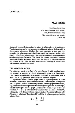
![THE ADJACENCY MATRIX 151
G: A = I 1 0 1
0 1 1 0
0 0 1 0
0 1 0 0
0 1 1 0
Fig. 13.1. A labeled graph and its adjacency matrix.
where A xx and A 22 are square. If A x and A 2 are adjacency matrices which
correspond to two different labelings of the same graph G, then for some
permutation matrix P9A x = P ~ lA 2P. Sometimes a labeling is irrelevant,
as in the following results which interpret the entries of the powers of the
adjacency matrix.
Theorem 13.1 Let G be a labeled graph with adjacency matrix A. Then the
i, j entry of Anis the number of walks of length n from to Vj.
Corollary 13.1(a) For i ^ j, the i, j entry of A 2 is the number of paths of
length 2 from vt to vy The i, i entry of A 2 is the degree of and that of A 3
is twice the number of triangles containing v£.
Corollary 13.1(b) If G is connected, the distance between and Vj for i ^ j
is the least integer n for which the i, j entry of Anis nonzero.
The adjacency matrix of a labeled digraph D is defined similarly: A =
.4(D) = [al7] has akj — 1 if arc VgVj is in D and is 0 otherwise. Thus A(D)
is not necessarily symmetric. Some results for digraphs using A(D) will
be given in Chapter 16. By definition of A(D the adjacency matrix of a
given graph can also be regarded as that of a symmetric digraph. We now
apply this observation to investigate the determinant of the adjacency
matrix of a graph, following [H27].
A linear subgraph of a digraph D is a spanning subgraph in which each
point has indegree one and outdegree one. Thus it consists of a disjoint
spanning collection of directed cycles.
Theorem 13.2 If D is a digraph whose linear subgraphs are Dh i = 1, • • •, n,
and Dt has e{even cycles, then
Every graph G is associated with that digraph D with arcs vpj and
whenever vtand Vj are adjacent in G. Under this correspondence, each linear
subgraph of D yields a spanning subgraph of G consisting of a point disjoint
collection of lines and cycles, which is called a linear subgraph of a graph.
n
det.4(D) = X ( - i r .
i= 1](https://image.slidesharecdn.com/graphtheory-181103155731/85/Graph-theory-162-320.jpg)
![152 MATRICES
Those components of a linear subgraph of G which are lines correspond to
the 2-cycles in the linear subgraph of D in a one-to-one fashion, but those
components which are cycles of G correspond to two directed cycles in D.
Since A{G) = A(D) when G and D are related as above, the determinant of
A(G) can be calculated.
Corollary 13.2(a) If G is a graph whose linear subgraphs are G,, i = 1
where G, has et even components and ct cycles, then
det A(G) = £ ( - 1 )e‘2Ci.
/= i
THE INCIDENCE MATRIX
A second matrix, associated with a graph G in which the points and lines are
labeled, is the incidence matrix B = [&jj. This p x q matrix has by = 1
if and Xj are incident and bu = 0 otherwise. As with the adjacency matrix,
the incidence matrix determines G up to isomorphism. In fact any p — 1
rows of B determine G since each row is the sum of all the others modulo 2.
The next theorem relates the adjacency matrix of the line graph of G to
the incidence matrix of G. We denote by BT the transpose of matrix B.
Theorem 13.3 For any (p, q) graph G with incidence matrix B,
A(L(G)) = BTB - 2Iq.
Let M denote the matrix obtained from —A by replacing the zth diagonal
entry by deg v{. The following theorem is contained in the pioneering work
of Kirchhoff [K7].
Theorem 13.4 (Matrix-Tree Theorem) Let G be a connected labeled graph
with adjacency matrix A. Then all cofactors of the matrix M are equal and
their common value is the number of spanning trees of G.
Proof. We begin the proof by changing either of the two l’s in each column
of the incidence matrix B of G to —1, thereby forming a new matrix E. (We
will see in Chapter 16 that this amounts to arbitrarily orienting the lines of
G and taking E as the incidence matrix of this oriented graph.)
The Uj entry of EET is en ejX + ei2eJ2 + • *• + eiqejq> which has the
value deg v( if i = j, —1 if v( and Vj are adjacent, and 0 otherwise. Hence
EEt = M.
Consider any submatrix of E consisting of p — 1 of its columns. This
p x (p — 1 ) matrix corresponds to a spanning subgraph H of G having
p - 1 lines. Remove an arbitrary row, say the fcth, from this matrix to
obtain a square matrix F of order p — 1. We will show that |det F is 1 or
0 according as H is or is not a tree. First, if H js not a tree, then because
H has p points and p — 1 lines, it is disconnected, implying that there is a](https://image.slidesharecdn.com/graphtheory-181103155731/85/Graph-theory-163-320.jpg)
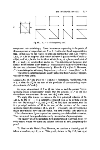
![154 MATRICES
Fig. 13.3. Two graphs with the same cycle matrix,
spanning trees, since the 2,3 cofactor, for example,
of M =
" 3 - 1 - 1 - 1"
- 1 2 - 1 0
- 1 - 1 3 - 1
- 1 0 - 1 2
is —
3 - 1 - 1
- 1 - 1 - 1
- 1 0 2
The number of labeled trees with p points is easily found by applying the
Matrix-Tree Theorem to K p. Each principal cofactor is the determinant
of order p — 1 :
p — 1 —1 • • * —1
- 1 p - 1 • • • - 1
- 1 - 1
Subtracting the first row from each of the others and adding the last p — 2
columns to the first yields an upper triangular matrix whose determinant
is pp~2.
Corollary 13.4(a) The number of labeled trees with p points is pp~2.
There appear to be as many different ways of proving this formula as
there are independent discoveries thereof. An interesting compilation of
such proofs is presented in Moon [M l5].
THE CYCLE MATRIX
Let G be a graph whose lines and cycles are labeled. The cycle matrix
C = [ c j of G has a row for each cycle and a column for each line with
Cij = 1 if the ith cycle contains line Xj and ctj = 0 otherwise. In contrast to
the adjacency and incidence matrices, the cycle matrix does not determine
a graph up to isomorphism. Obviously the presence or absence of lines
which lie on no cycle is not indicated. Even when such lines are excluded,
however, C does not determine G, as is shown by the pair ofgraphs in Fig. 13.3,](https://image.slidesharecdn.com/graphtheory-181103155731/85/Graph-theory-165-320.jpg)
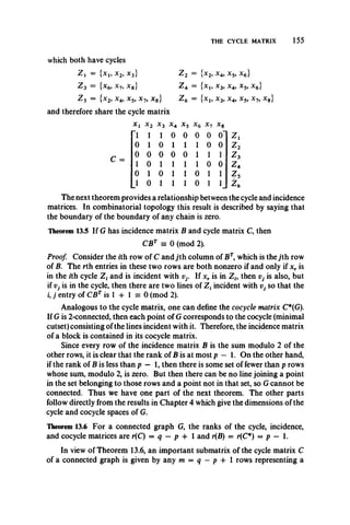
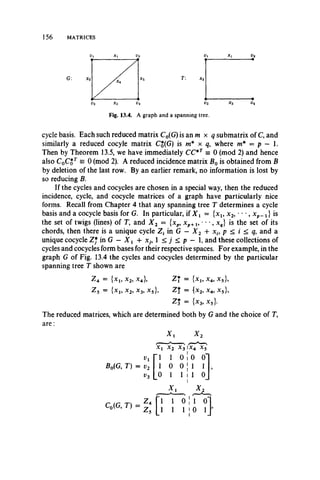
![THE CYCLE MATRIX 157
an d X { X 2
z* 'i 0 0 1 1“
C%(G, T) = Z* 0 1 0 1 1
z t 0 0 1 0 1
It is easy to see that this is a special case of the following equations (all
modulo 2) which hold for any connected graph G and spanning tree T :
Xi x2 *2
£ 0 = f*0(G, T) = K f lj, C0 = C0(G, T) = [Ci 7 j ,
and
& * 2
C% = CJ(G, T) = £ CJ1
where C[ = B l 1B2 = C and CJ = B i lB0 = [ /w* C []. It follows from
these equations that, given G and T, each of the partitioned matrices £ 0,
C0, and CJ determines the other two.
Excursion—Matroids Revisited
The cycle and cocycle matrices are particular representations of the cycle
matroid and cocycle matroid of a graph, introduced in Chapter 4. A matroid
is called graphical if it is the cycle matroid of some graph, and cographical if it
is a cocycle matroid. Tutte [T12] has determined which matroids are
graphical or cographical, thereby inadvertently solving a previously open
problem in electric network theory.
The smallest example ofa matroid which is not graphical or cographical is
the self-dual matroid obtained by taking M = {1, 2, 3, 4} and the circuits
all 3-element subsets of Af.
Fig. 13.5. The new circuits in the whirl of W5.
Another example, Tutte [T19], of a matroid which is not graphical
involves the wheel Wn+l = + C„. Its cycle matroid has n2 — n 4-1
circuits since there are that many cycles in a wheel. If in this matroid we
remove from the collection of circuits the cycle C„ which forms the rim of the
wheel, and add to it all of the “spoked rims” (the sets of lines in the subgraphs
shown in Fig. 13.5), then it can be shown that the result is a new matroid](https://image.slidesharecdn.com/graphtheory-181103155731/85/Graph-theory-168-320.jpg)
![158 MATRICES
which is not graphical or cographical. This is called a whirl of order n and is
generated by n2 circuits.
Even if a matroid is graphical, it need not be cographical. For example,
the cycle matroid of K 5is not cographical. In fact a matroid is both graphical
and cographical if and only if it is the cycle matroid of some planar graph.
EXERCISES
13.1 a) Characterize the adjacency matrix of a bipartite graph.
b) A graph Gis bipartite ifand only iffor all odd nevery diagonal entry of A*is 0.
13.2 Let G be a connected graph with adjacency matrix A. What can be said about A if
a) is a cutpoint?
b) is a bridge?
13.3 If cn(G) is the number of w-cycles of a graph G with adjacency matrix A, then
a) c3(G) = |tr(/43).
b) c4(G) = i[tr(/44)- 2q - 2 I i#, <?>].
c) cs(G) = M trM 5)- 5 tr(/43) - 5 I f . au - 2)«<,3>].
(Harary and Manvel [HM1])
13.4 a) If G is a disconnected labeled graph, then every cofactor of M is 0.
b) If G is connected, the number of spanning trees of G is the product of the
number of spanning trees of the blocks of G.
(Brooks, Smith, Stone, and Tutte [BSST1])
13.5 Let G be a labeled graph with lines xl9x2, *• *, xq. Define the p x p matrix
M x = [my] by
( - x k if xk = v,vj
m{j = < for i # y,
(0 if Vi and Vj are not adjacent
-m u = X«i»-
n*/
By the term ofa spanning tree of Gis meant the product ofits lines. The tree polynomial
of G is defined as the sum of the terms of its spanning trees.
The Variable Matrix Tree Theorem asserts that the value of any cofactor of the
matrix Mx is the tree polynomial of G.
13.6 Do there exist two different graphs with the same cycle matrix which are smaller
than those in Fig. 13.3?
13.7 The “cycle-matroid” and “cocycle-matroid” of a graph do indeed satisfy the
first definition of matroid given in Chapter 4.
13.8 Two graphs G{ and G2 are cospectral if the polynomials det(/4t - tl) and
det (A2 — tl) are equal. There are just two different cospectral graphs with 5 points.
(F. Harary, C. King, and R. C. Read)
13.9 If the eigenvalues of A(G) are distinct, then every nonidentity automorphism of
G has order 2. (Mowshowitz [M l7])](https://image.slidesharecdn.com/graphtheory-181103155731/85/Graph-theory-169-320.jpg)
![EXERCISES 159
13.10 Let f(t) be a polynomial of minimum degree (if any) such that every entry of
f(A) is 1, where A is the adjacency matrix of G. Then a graph has such a polynomial if
and only if it is connected and regular. (Hoffman [H45])
13.11 An eulerian matroid has a partition of its set S of elements into circuits.
a) A graphical matroid is eulerian if and only if it is the cycle matroid of an
eulerian graph,
b) Not every eulerian matroid is graphical.
13.12 In a binary matroid, the intersection of every circuit and cocircuit has even
cardinality. Every cocircuit of a binary eulerian matroid has even cardinality. In other
words, the dual ofa binary eulerian matroid is a “bipartite matroid,”defined as expected.
(Welsh [W9])](https://image.slidesharecdn.com/graphtheory-181103155731/85/Graph-theory-170-320.jpg)
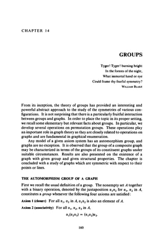
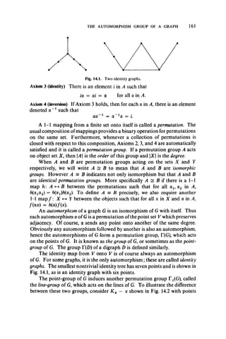
![162 GROUPS
Fig. 14.2. A graph with labeled points and
lines.
K 4- x :
labeled vl9 v2, v3, v4 and lines x l9 x2, x3, x4, x5. The point-group r(X 4 - x)
consists of the four permutations:
f o l^ X ^ ) -
The identity permutation of the point-group induces the identity
permutation on the lines, while induces a permutation on the
lines which fixes x5, interchanges x x with x4 and x2 with x3. In this way, one
sees that the line-group r t(K4 - x) consists of the following permutations,
induced respectively by the above members of the point-group:
( * lX * 2X * 3X *4X * 5), (x i X4 ) { x 2X3)(x 5), ( x 1X2X x 3X4K x 5), f o x ^ ^ ^ X ^ ) -
Of course the line-group and the point-group of K4 — x are isomorphic.
But they are certainly not identical permutation groups since TX(K4 —x)
has degree 5 and T(K4 —x) has degree 4. Note that the line x 5 is fixed by
every member of the line-group. Even the permutation group obtained from
Tl(K4 —x) by restricting its object set to x l9 x 2, x3, x4 is not identical with
r(K4 — x), since these two isomorphic permutation groups of the same
degree have different cycle structure. Furthermore, it can be shown that
even when two permutation groups have the same degree and the same cycle
structure, they still need not be identical; see Polya [P5, p. 176].
The next theorem [HP15] answers the question: when are T(G) and
r^G ) isomorphic? Sabidussi [SI] demonstrated the sufficiency using group
theoretic methods.
Theorem 14.1 The line-group and the point-group ofa graph Gare isomorphic
if and only if G has at most one isolated point and K2 is not a component
Proof. Let a' be the permutation in T t(G) which is induced by the permuta
tion a in T(G). By the definition of multiplication in T^G), we have
for all a, /? in T(G). Thus the mapping a a' is a group homomorphism
from T(G) onto T^G). Hence T(G) ^ T^G) if and only if the kernel of this
mapping is trivial.
To prove the necessity, assume T(G) s T^G). Then a ^ i (the identity
permutation) implies a' ^ i. If G has distinct isolated points vt and vl9 we
can define a e T(G) by a ^ ) = i?2, ct{v2) = vl9 and a(y) = v for all v ^ vi9 v2.
of G.
a'/r = m](https://image.slidesharecdn.com/graphtheory-181103155731/85/Graph-theory-173-320.jpg)
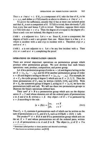
![164 GROUPS
Table 14.1
OPERATIONS ON PERMUTATION GROUPS
Sum Product Composition Power
group A B A + B A x B AIS] BA
objects X Y X u Y X x Y X x Y y X
order m n mn mn mnd mn
degree d e d + e de de ed
permuted by a x p as expected:
(a x p)(x, y) = (ax, py). (14.2)
The product C3 x S2 also has order 6 but while the degree of the sum
C3 + S2 is 5, that of the product is 6 . The permutation in C3 x S2 corre
sponding to (123) + (ab) in the sum is (la 26 3a lb 2a 3b), where for brevity
la denotes (1, a).
The compassion* y4[J9] o f a r o u n d IT also acts on x Y. For each a
in A and any sequence (Pl9 P2, " , Pd)°f ^ (not necessarily distinct) permuta
tions in B, there is a unique permutation in A[B] written (a; p l9 P2, ', Pd)
such that for (xif yy) in X x Y :
(a ; P u P * ' * *, y j ) = (a *i> &>>;)• (14.3)
The composition C3[S2] has degree 6 but its order is 24. Each permutation
in C3[S2] may be written in the form in which it acts on X x Y. Using the
same notation la for the ordered pair (1, a) and applying the definition (14.3),
one can verify that ((123); (a)(6), (a6), (aX6)) is expressible as (la 2a 36 16 26 3a).
Note that S2[C 3] has order 18 and so is not isomorphic to C3[S2].
The power group** denoted by BA acts on Yx, the set of all functions
from X into Y. We will always assume that the power group acts on more than
one function. For each pair of permutations a in A and P in B there is a
unique permutation, written p* in BA. We specify the action of pa on any
function / in Yx by the following equation which gives the image of each
x g X under the function /?*/:
(/?“/)(x) = Pf(*x). (14.4)
The power group S23has order 6 and degree 8. It is easy to see by applying
(14.4) that the permutation in this group obtained from a = (123) and
p = (a6) has one cycle of length 2 and one of length 6 .
Table 14.1 summarizes the information concerning the order and degree
of each of these four operations.
* Called “Gruppenkranz” by Polya[P6] and “wreath product” by Littlewood [L3] and others.
** Not called by any other name as yet.](https://image.slidesharecdn.com/graphtheory-181103155731/85/Graph-theory-175-320.jpg)
![THE GROUP OF A COMPOSITE GRAPH 165
Table 14.2
PERMUTATION GROUPS OF DEGREE p
Symbol Order Definition
Symmetric S, p! All permutations on {1, 2, • • • ,/>}
Alternating *p p!2 All even permutations on {1, 2, • • • ,/?}
Cyclic c . P Generated by (12 • • •p)
Dihedral 2P Generated by (12 • •p) and (lp)(2 p—1) • • •
Identity Ep 1 (1)(2) • • • (p) is the only permutation.
We now see that three of these operations are not all that different.
Theorem 14.2 The three groups A -b B, A x £, and BA are isomorphic.
It is easy to show that A + B s A x B. To see that A + B s BA, we
define the map / : BA -►A + B by /(a ; fi) = a " 1/!, and verify that / is an
isomorphism. Note that these three operations are commutative; in fact,
A + B = B + A , A x B = B x A9and BA = A8.
Table 14.2 introduces notation for five well-known permutation groups
of degree p. In these terms, we can describe the groups of two familiar
graphs with p points.
Theorem 14.3 a) The group T(G) is Sp if and only if G = K p or G = K p.
b) If G is a cycle of length p, then T(G) = Dp.
Thus two particular permutation groups of degree p, namely Sp and Dp,
belong to graphs with p points. For all p > 6, there exists an identity graph
with p points and in fact whenever p > 7, there is an identity tree.
THE GROUP OF A COMPOSITE GRAPH
Now we are ready to study the group associated with a graph formed from
other graphs by various operations. Since every automorphism of a graph
preserves both adjacency and nonadjacency, an obvious but important
result immediately follows.
Theorem 14.4 A graph and its complement have the same group,
n o = T(G). (14.5)
A “composite graph” is the result of one or more operations on disjoint
graphs. The group of a composite graph may often be expressed in terms of
the groups of the constituent graphs. Frucht [F10] described the group of
a graph nG which consists of n disjoint copies of a connected graph G.](https://image.slidesharecdn.com/graphtheory-181103155731/85/Graph-theory-176-320.jpg)
![T(nG) = SJT(G)]. (14.6)
To illustrate the theorem, consider the graph G = 5K3, whose group is
^ 5[S3]. An automorphism of G can always be obtained by performing an
arbitrary automorphism on each of the five triangles, and then following this
by any permutation of the triangles among themselves.
Theorem 14.6 If Gx and G2 are disjoint, connected, nonisomorphic graphs,
then
r(G j u G2) s n G x) 4- r(G 2). (14.7)
Any graph G can be written as G = HjGj u n2G2 u • • • u nrGr, where
nt is the number of components of G isomorphic to Gf. Applying the last
two theorems, we have the result,
n o = s ni[r(G ,)] + s„2[r(G 2)] + • • • + s j n c , ) ] . (14.8)
Corollary 14.6(a) The group of the union of two graphs is the sum of their
groups,
T(GXu G2) se T(GX) + T(G2), (14.9)
if and only if no component of Gx is isomorphic with a component of G2.
The next corollary follows from Theorem 14.4, the preceding corollary,
and the fact that the complement of the join of two graphs is the union of
their complements, that is,
Gi + G2 = Gx u G2. (14.10)
Corollary 14.6(b) The group of the join of two graphs is the sum of their
groups,
HGj + G2) = IXGj) + T(G2), (14.11)
if and only if no component of Gi is isomorphic with a component of G2.
A nontrivial graph G is prime if G = Gx x G2 implies that Gt or G2 is
trivial; G is composite if it is not prime. Sabidussi [S5] observed that the
cartesian product of graphs is commutative and associative. He also devel
oped a criterion for the group of the product of two graphs to be the product
of their groups. Since he proved that every nontrivial graph is the unique
product of prime graphs, the meaning of relatively prime graphs is clear.
Theorem 14.7 The group of the product of two graphs is the product of their
groups,
T(Gj x G2) = HGj) x T(G2), (14.12)
if and only if Gx and G2 are relatively prime.
Sabidussi [S4] settled the question raised in [H21] by providing a
criterion for the group of the lexicographic product (composition) of two
166 GROUPS
Theorem 14.5 If G is a connected graph, then](https://image.slidesharecdn.com/graphtheory-181103155731/85/Graph-theory-177-320.jpg)
![THE GROUP OF A COMPOSITE GRAPH 167
Table 14.3
THE GROUPS OF THE LITTLE CONNECTED GRAPHS
graphs to be the composition oftheir groups. The neighborhood ofa point u is
the set N(u) consisting of all points v which are adjacent with u. The closed
neighborhood is N[u~ = N(u) u {«}.
Theorem 14.8 If Gxis not totally disconnected, then the group of the composi
tion of two graphs Gx and G2 is the composition of their groups,
H G ^G J) s r(G1)[r(G2)], (14.13)
if and only if the following two conditions hold:
1. If there are two points in Gt with the same neighborhood, then G2 is
connected.
2. If there are two points in with the same closed neighborhood, then
G2 is connected.
With these results, the groups of all graphs with p < 4 points can be
symbolized. The group of one of these graphs, namely K 4 —x, has already
been illustrated. The groups of the disconnected graphs are not given in
Table 14.3 but can be obtained by using Theorem 14.4.
The conditions for the group of the lexicographic products of two
graphs to be identical to the composition of their groups are rather complex.
This suggests that another operation on graphs be constructed for the purpose
of realizing the composition of their groups only up to group isomorphism.
The corona Gt ° G2 of two graphs Gx and G2 was defined by Frucht and
Harary [FH1] as the graph G obtained by taking one copy of Gx (which has](https://image.slidesharecdn.com/graphtheory-181103155731/85/Graph-theory-178-320.jpg)
![168 GROUPS
Gx°
AFig. 14.3. Two graphs and their two coronas.
px points) and px copies of G2, and then joining the ith point of Gx to every
point in the zth copy of G2. For the graphs Gx = K 2 and G2 = K l 2, the
two different coronas Gx° G2 and G2 ° Gx are shown in Fig. 14.3. It follows
from the definition of the corona that Gx° G2 has px(1 4- p2) points and
qx + pxq2 + P1P2 lines.
Theorem 14.9 The group of the corona of two graphs Gx and G2 can be
written explicitly in terms of the composition of their groups,
if and only if Gj or G2 has no isolated points.
The term E x in (14.14) when applied to Corollary 14.6(a) gives the
next result.
Corollary 14.9(a) The group of the corona Gx o G2 of two graphs is isomorphic
to the composition r(G 1)[T(G2)] of their groups if and only if Gx or G2 has
no isolated points.
GRAPHS WITH A GIVEN GROUP
Konig [K10, p. 5] asked: When is a given abstract group isomorphic with
the group of some graph? An affirmative answer to this question was given
constructively by Frucht [F 8]. His proof that every group is the group of
some graph makes use of the Cayley “color-graph of a group” [C4] which we
now define. Let F = {/0, f u •••, f n_ x} be a finite group of order n whose
identity element is / 0. Let each nonidentity element / in F have associated
with it a different color. The color-graph of F, denoted D(F is a complete
symmetric digraph whose points are the n elements of F. In addition, each
arc of D(F), say from / to f j9 is labeled with the color associated with the
element f f V} of F. Of course, in practice we simply label both points and
arcs of D(F) with the elements of F.
For example, consider the cyclic group of order 3, C3 = {0, 1, 2}. The
color-graph Z)(C3) is shown in Fig. 14.4.
Frucht observed the next result, which is simple but very useful.
r(G, o g 2) = nG jp, + r(G2)], (14.14)](https://image.slidesharecdn.com/graphtheory-181103155731/85/Graph-theory-179-320.jpg)
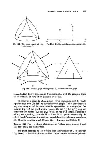
![170 GROUPS
any graph so constructed is excessive. Graphs with a given group and fewer
points can be obtained when the group is known to have m < n generators.
In that case the color-graph is modified to include only directed lines which
correspond to the m generators. Thus a graph containing n(m -f- 1)(2m -f 1)
points can be obtained for the given group. Since C3 can be generated by
one element, there is a graph with 18 points for C3. It is shown in Fig. 14.6(b).
Fig. 14.7. The smallest graph whose group
is Cy
The inefficiency of even this improvement of the method of construction
is shown by the graph of Fig. 14.7. This is the unique smallest graph
whose automorphism group is cyclic of order three [HP3] and it has only
9 points and 15 lines.
Later Frucht [F9] showed that one could also specify that G be cubic.
It was becoming apparent that requiring G to have a given abstract group of
automorphisms was not a severe restriction. In fact Sabidussi [S2] showed
that there are many graphs with a given abstract group having one of several
other specified properties such as connectivity, chromatic number, and
degree of regularity.
Theorem 14.11 Given any finite, abstract, nontrivial group F and an integer
j (1 < j < 4), there are infinitely many nonhomeomorphic graphs G such
that G is connected, has no point fixed by every automorphism, T(G) = F,
and G also has the property Pp defined by
P {: k(G) = n, n > 1
Pi ' X(G) = n, n > 2
P3: G is regular of degree n, n > 3
P4: G is spanned by a subgraph homeomorphic to a given graph.
When Theorem 14.11 was published, Izbicki [II] looked into the problem
of constructing a graph with a given group which satisfies several of these
conditions simultaneously. By exploiting the results of Sabidussi [S2]
on the product of two graphs and making some constructions, he was able
to obtain a corresponding result involving regular graphs of arbitrary
degree and chromatic number.](https://image.slidesharecdn.com/graphtheory-181103155731/85/Graph-theory-181-320.jpg)
![SYMMETRIC GRAPHS 171
Corollary 14.11(a) Given any finite group F and integers n and m where
n > 3 and 2 < m < n, there are an infinite number of graphs G such that
T(G) ~ F, x(G) = m, and G is regular of degree n.
SYMMETRIC GRAPHS
The study of symmetry in graphs was initiated by Foster [F6], who made
a tabulation of symmetric cubic graphs. Two points u and v of the graph G
are similar if for some automorphism a of G, ol{u ) = v. Afixed point is not
similar to any other point. Two lines x x = UiVx and x 2 = u2v2 are called
similar if there is an automorphism a of G such that a({wl5 vx}) = {u2, v2}.
We consider only graphs with no isolated points. A graph is point-symmetric
if every pair of points are similar; it is line-symmetric if every pair of lines are
similar; and it is symmetric if it is both point-symmetric and line-symmetric.
The smallest graphs that are point-symmetric but not line-symmetric
(the triangular prism K 3 x K 2) and vice versa (the star K 12) are shown in
Fig. 14.8.
Fig. 14.8. A point-symmetric and a line-symmetric graph.
Note that if a is an automorphism of G, then it is clear that G — u and
G — a(n) are isomorphic. Therefore, if u and v are similar, then G — u =
G — v. Surprisingly, the converse of this statement is not true.* The graph
in Fig. 14.9 provides a counterexample. It is the smallest graph which has
dissimilar points u and v such that G — u £ G —v, see [HP5].
The degree of a line x = uv is the unordered pair (du d2) with
dx = deg m, and d2 = deg v. A graph is line-regular if all lines have the
same degree. In Fig. 14.10, the complete bipartite graph K 2 3 is shown; it is
line-symmetric but not point-symmetric and is line-regular of degree (2, 3).
* A purported proof of Ulam’s conjecture depended heavily on this converse.](https://image.slidesharecdn.com/graphtheory-181103155731/85/Graph-theory-182-320.jpg)
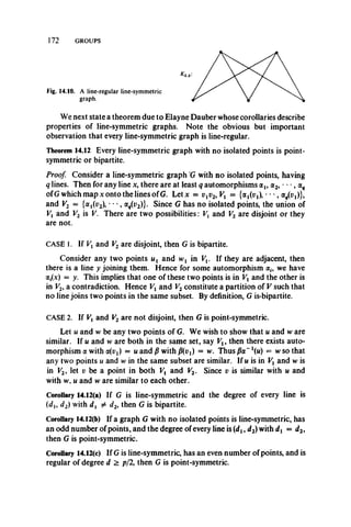
![HIGHLY SYMMETRIC GRAPHS 173
With these three corollaries, the only line-symmetric graphs not yet
characterized are those having an even number of points which are regular
of degree d < p/2. The polygon with six points is an example of such a
line-symmetric graph which is both point-symmetric and bipartite. The
icosahedron, the dodecahedron, and the Petersen graph are examples of
such line-symmetric graphs which are point-symmetric but not bipartite.
But not all regular line-symmetric graphs are point-symmetric, as Folkman
[F5] discovered.
Theorem 14.13 Whenever p > 20 is divisible by 4, there exists a regular
graph G with p points which is line-symmetric but not point-symmetric.
HIGHLY SYMMETRIC GRAPHS
Following Tutte [T20], an n-route is a walk of length n with specified initial
point in which no line succeeds itself. A graph G is n-transitive, w > 1, if it
has an n-route and if there is always an automorphism of G sending each
n-route onto any other n-route. Obviously a cycle ofany length is n-transitive
for all n, and a path of length n is n-transitive. Note that not every line-sym
metric graph is 1-transitive. For example, in the line-symmetric graph
K x>2 of Fig. 14.8, there is no automorphism sending the 1-route uv onto the
1-route vw.
If W is an n-route v0 vx • *- v„and u is any point other than vn_ x adjacent
with vn, then the n-route vx • • *vnu is called a successor of W. If W terminates
in an endpoint of G, then obviously W has no successor. For this reason, it
is specified in the next two theorems that G is a graph with no endpoints. We
now have a sufficient condition [T20, p. 60] for n-transitivity.
Theorem 14.14 Let G be a connected graph with no endpoints. If W is an
n-route such that there is an automorphism of G from W onto each of its
successors, then G is n-transitive.
There is a straightforward relationship [T20, p. 61] between n-transitivity
and the girth of a graph.
Theorem 14.15 If G is connected, n-transitive, is not a cycle, has no endpoints
and has girth g, then n < 1 4- g/2.](https://image.slidesharecdn.com/graphtheory-181103155731/85/Graph-theory-184-320.jpg)
![174 GROUPS
Using Theorem 14.14, it can be shown that the Heawood graph in
Fig. 14.11 is 4-transitive. Furthermore, it is easily seen from Theorem 14.15
that this graph is not 5-transitive.
There are regular graphs called “cages” which are, in a sense, even more
highly symmetric than n-transitive graphs. A graph G is n-unitransitive* ifit is
connected, cubic, and n-transitive, and if for any two n-routes Wx and W2,
there is exactly one automorphism a of G such that olWx = W2. An n-cage,
n > 3, is a cubic graph of girth n with the minimum possible number of
points. Information about cages is presented in the next statement
[T20, pp. 71-83].
Fig. 14.12. The 7-cage is the union of the above subgraphs as labeled.
Fig. 14.13. The 8-cage is the union of the above subgraphs as labeled.
* Called n-regular in[T20, p. 62].](https://image.slidesharecdn.com/graphtheory-181103155731/85/Graph-theory-185-320.jpg)
![HIGHLY SYMMETRIC GRAPHS 175
Table 14.4
THE KNOWN CAGES
n The w-cage n The «-cage
3 K4 (shown in Fig. 2.1) 6 Heawood graph (Fig. 14.11)
4 * 3,3 (Fig. 2.5) 7 McGee graph (Fig. 14.12)
5 Petersen graph (Fig. 9.6) 8 Levi graph (Fig. 14.13)
Theorem 14.16 There exists an n-cage for all n > 3. For n = 3 to 8 there is
a unique n-cage. Each of these n-cages is t-unitransitive for some t = t(n),
namely, t{3) = 2, t(4) = f(5) = 3, t(6) = r(7) = 4, and f(8) = 5.
All the known cages are now specified.
There are no n-transitive cubic graphs for n > 5, hence no n-unitransitive
ones; see Tutte [T8]. However, there are other n-unitransitive graphs,
n < 5, in addition to the cages. In particular, Frucht [F ll] constructed
a 1-unitransitive graph of girth 12 with 432 points, the cube Q3 and the
dodecahedron (Fig. 1.5) are 2-unitransitive, and Coxeter [CIO] found 3-
unitransitive graphs other than the 4-cage and 5-cage. One of these is
shown in Fig. 14.14.
This graph is a member of a class of graphs defined in [CH3]. For any
permutation a in Sp, the a-permutation graph of a labeled graph G is the
union of two disjoint copies Gx and G2 of G together with the lines joining
point vt of Gj with va{i) of G2. Thus Fig. 14.14 shows a permutation graph
of the cycle C10. The front cover of this book shows all four permutation
graphs of C5.](https://image.slidesharecdn.com/graphtheory-181103155731/85/Graph-theory-186-320.jpg)
![176 GROUPS
m.m
EXERCISES
14.1 Find the groups of the following graphs: (a) 3K 2, (b) K 2 -f C4, (c) K m
(<*) * i.2[* 2l (c) K4 u C4.
14.2 If a connected graph G has a point which is not in a cycle of length four, then G
is prime. (Sabidussi [S2])
14.3 Let G be connected with p > 3. Then L(G) is prime if and only if G is not Kmn
for m, n > 2. (Palmer [PI j)
14.5 Construct a connected graph with 11 points whose group is cyclic of order 6.
14.6 Construct a graph with 14 points whose group is cyclic of order 7.
(Sabidussi [S3])
*14.7 Let c(m) be the smallest number of points in a graph whose group is isomorphic
to Cm. Then the values of c(m) for m — nr and n prime are
a) c(2) = 2, and c(2r) = 2r + 6 when r > 1.
b) c(nr) = tf + 2n for n = 3,5.
c) c{nr) = nr -f n for n > 7.
[Note: c(m) can be calculated when m is not a prime power, but the expression is
complicated.] (R. L. Meriwether)
14.8 There are no nontrivial identity graphs with less than 6 points.
14.9 There are no cubic identity graphs with less than 12 points.
14.10 Construct a cubic graph whose group is cyclic of order 3.
14.11 The group of the Petersen graph is identical to the line-group of Ks.
14.12 There exists a graph G whose group is the dihedral group Dpsuch that G is not
a cycle or its complement. What is the smallest value of p for which this holds?
14.13 For p > 3 there are no graphs G such that T(G) = Apor Cp. And when p > 4
there are no digraphs D with T(D) = Ap. (Kagno [K l], Harary and Palmer [HP10])
14.14 The only connected graph with group isomorphic to Sn, n > 3,
a) with n points is K„,
b) with n 4-1 points is K l n,
c) with n + 2 points is 4- Kl n. (Gewirtz and Quintas [GQ1])
14.15 Given a finite group F, let G(F) be the graph obtained by Frucht’s Theorem.
Then every nonidentity automorphism of G(F) leaves no point fixed.
14.16 What is the smallest tree T containing dissimilar points u and v such that
T - u ^ T — v? (Harary and Palmer [HP2])
14.17 Every connected, point-symmetric graph G is a block.
14.18 A starred polygon is a graph G containing a spanning cycle v l v2 m” vp
such that whenever the line vmvm+„ is in G, so are all lines vtVjwherej — i = n(mod p). A
connected graph with a prime number p of points is point-symmetric if and only if it is
a starred polygon. (Turner [T4])
14.19 Prove or disprove the following eight statements: If two graphs are point-
symmetric (line-symmetric), then so are theirjoin, product, composition, and corona.](https://image.slidesharecdn.com/graphtheory-181103155731/85/Graph-theory-187-320.jpg)
![EXERCISES 177
1420 Every symmetric, connected graph of odd degree is 1-transitive.
(Tutte [T20, p. 59])
1421 Every symmetric, connected, cubic graph is n-transitive for some n.
(Tutte [T20, p. 63])
1422 Find necessary and sufficient conditions for the point-group and line-group of a
graph to be identical. (Harary and Palmer [HP15])
1423 If Gis connected, then T(G) s T(L(G)) if and only if G # K2, * i,3 + x , * 4 - x ,
or * 4. (Whitney [W11])
1424 If G is point-symmetric, then if T(G) is abelian, it is a group of the form
S2 + S2 + ••• + S2. (McAndrew [M8])
14.25 The only doubly transitive graphical permutation group of degree p is Sp.
14.26 Let A and B be two permutation groups acting on the sets * = {xl5 x2, ' **, xd}
and Y respectively. The exponentiation group, denoted [B]'4, acts on the functions
Yx. For each permutation a in A and each sequence of permutations /?2, • ••,
in B there is a unique permutation [a; /?2, • ••, in [B]A such that for x, in *
and /in Yx
[a; jg„ /?2, •■•, i) =
Then the group of the cube Q„is [S2]s"and the line-group of K„„is [S„]Sj.
(Harary [H18])
*14.27 There exists a unique, smallest graph of girth 5 which is regular of degree 4. It
has 19 points and its group is isomorphic to the dihedral group D12.
(Robertson [R18])
1428 Let G be a triply connected planar (p, q) graph whose group has order s. Then
4q/s is an integer and s = 4q if and only if G is one of the five platonic graphs.
(Weinberg [W8], Harary and Tutte [HT4])
14.29 The group of any tree can be obtained from symmetric groups by the operations
of sum and composition. (Polya [P5, p. 209])
14.30 A collection of p — 1 transpositions (ux t^), (u2v2), •*• on p objects generates
the symmetric group Spif and only if the graph with p points and the p — 1 lines u& is
a tree. (Polya [P5])
14.31 The a-permutation graph of a labeled 2-connected graph G is planar if and only
if G is outerplanar and can be drawn in the plane with a cyclic labeling of its points so
that a is in the dihedral group Dp. (Chartrand and Harary [CH3])
*14.32 An endomorphism of G is a homomorphism from G into itself. The semigroup
ofa graph is the collection of all its endomorphisms. Every finite semigroup with unit
is isomorphic with the semigroup of some graph. (Hedrlin and Pultr [HP23])
*1433 The smallest nontrivial graph having only the identity endomorphism has 8
points. (Hedrlin and Pultr [HP24J)](https://image.slidesharecdn.com/graphtheory-181103155731/85/Graph-theory-188-320.jpg)
![C H A P T E R 15
ENUMERATION
How do I love thee? Let me count the ways.
E l iz a b e t h B a r r e t t B r o w n i n g
There is something to be said for regarding enumerative methods in com
binatorial analysis as more of an art than a science. With the discovery and
development of more general and powerful viewpoints and techniques, it is
to be hoped that this situation will become reversed. The pioneers in
graphical enumeration theory were Cayley, Redfield, and Polya. In fact,
as noted in [HP11], all graphical enumeration methods in current use were
anticipated in the unique paper by Redfield [R8] published in 1927 but
unfortunately overlooked.
We begin with the easiest enumeration problems, those for labeled graphs.
We then present Polya’s classical enumeration theorem and use it to derive
counting series for trees and various other kinds of graphs. Polya’s theorem
has been generalized to the Power Group Enumeration Theorem which is
useful for certain counting problems where the equivalence classes are
determined by two permutation groups. For the sake of completeness, we
conclude with lists of both solved and unsolved problems in graphical
enumeration.
LABELED GRAPHS
All of the labeled graphs with three points are shown in Fig. 15.1. We
see that the 4 different graphs with 3 points become 8 different labeled
graphs. To obtain the number of labeled graphs with p points, we need
only observe that each of the (5) possible lines is either present or absent.
Theorem 15.1 The number of labeled graphs with p points is 2 .
178](https://image.slidesharecdn.com/graphtheory-181103155731/85/Graph-theory-189-320.jpg)
![LABELED GRAPHS 179
v2m
l>3 ^ 2 ^
• U3 V 2«
Fig. 15.1. The labeled graphs with three points.
Corollary 15.1(a) The number of labeled (p, q) graphs is
Cayley [C6] was the first to state the corresponding result for trees:
The number of labeled trees with p points is pp” 2. Since 1889, when Cayley’s
paper appeared, many different proofs have been found for obtaining his
formula. Moon [M l5] presents an outline of these various methods of
proof, one of which was given in Corollary 13.4(a).
In Fig. 15.2 are all the 16 labeled trees with 4 points. The labels on these
trees are understood to be as in the first and last trees shown. We note
that among these 16 labeled trees, 12 are isomorphic to the path PA and 4
to K l 3. The order of r(jP4) is 2 and that of T(KX3) is 6. We observe that
since p = 4 here, we have 12 = 4!/|T(P4)| and 4 = 4!/|r(X1>3)|. The
Fig. 15.2. The labeled trees with four points.](https://image.slidesharecdn.com/graphtheory-181103155731/85/Graph-theory-190-320.jpg)
![180 ENUMERATION
expected generalization of these two observations holds not only for trees,
but also for graphs, digraphs, relations, and so forth;see [HR1] and [HPR1],
Theorem 15.2 The number of ways in which a given graph G can be labeled
isp!/|r(G)|.
Outline ofproof Let A be a permutation group acting on the set X of objects.
For any element x in X , the orbit of x, denoted 0(x), is the subset of X which
consists of all elements y in X such that for some permutation a in A, ax = y.
The stabilizer of x, denoted A(x is the subgroup of A which consists of all
the permutations in A which leave x fixed. The result follows from an
application of the well-known formula |0(x)| •|y4(x )| = A and its inter
pretation in the present context.
POLYA’S ENUMERATION THEOREM
Many enumeration problems are formulated in such a way that the answer
can be given by finding a formula for the number of orbits (transitivity
systems) determined by a permutation group. Often, weights are assigned
to the orbits and Polya [P5] showed how to obtain a formula which enumer
ates the orbits according to weight and which depends on the cycle structure
of the permutations in the given group. Polya’s theorem in turn depends on
a generalization of a well-known counting formula due to Burnside
[B20, p. 191].
Theorem 15.3 Let A be a permutation group acting on set X with orbits
01, 62, * *•,0„, andlet vv.be a function which assigns a weightto each orbit.
Furthermore, vvis defined on X so that w(x) = w(0,) whenever x € 0,. Then
the sum of the weights of the orbits is given by
Mli MOi) =Z! Z (151)
i = 1 aeA x = ax
Proof We have already seen that the orderA of the group A is the product
|/l(x)| • |0(x)| for any x in X, where A(x) is the stabilizer of x. Also, since the
weight function is constant on the elements in a given orbit, we see that
10.1 w(0|) = X Mx),
xe0,
for each orbit 0,. Combining these facts, we find that
Ml MOi) = XMWI Mx).
X€0i
Summing over all orbits, we have
MlZ MOi) =Z Z MMI w(*)>
i - 1 i = 1 xeOi
from which (15.1) follows readily.](https://image.slidesharecdn.com/graphtheory-181103155731/85/Graph-theory-191-320.jpg)
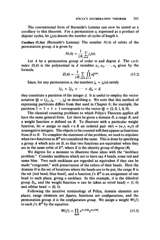
![182 ENUMERATION
It is easy to see that each function in a given orbit of RDunder EA has the
same weight, so that the weight of an orbit can be defined as the weight of
any function in it.
Suppose there are cmn figures of weight (m, n) in R and Cmn orbits
(equivalence classes of configurations) of weight xmyn in RD. The figure
counting series
c(x,y) = Y ,cmnXmyH (15.4)
enumerates the elements of R by weight, and the configuration counting
C (x j) = I W (15.5)
is the generating function for equivalence classes of functions. Polya’s
Theorem [P5] expresses C(x, y) in terms of c(x, y).
If in (15.2) we write Z(A) = Z (A ; au a2, • • •, ad), then for any function
h(x, y), we define
Z (A h(x, y)) = Z (A ; h(x, y h(x y2), • •, h(xd9/)). (15.6)
Theorem 15.4 (Polya’s Enumeration Theorem) The configuration counting
series is obtained by substituting the figure counting series into the cycle
index of the configuration group,
C(x, y) = Z(A, c(x, y)). (15.7)
Proof. Let a be a permutation in A, and let a be the corresponding permuta
tion in the power group EA. Assume first that / is a configuration fixed by
a and that £ is a cycle of length k in the disjoint-cycle decomposition of a.
Then f(b) = /(£b) for every element b in the representation of £, so that all
elements permuted by £ must have the same image under f Conversely,
if the elements of each cycle of the permutation a have the same image under
a configuration f then a fixes f Therefore, all configurations fixed by £
are obtained by independently selecting an element r in R for each cycle £ of
a and setting/(b) = r for all b permuted by £. Then if the weight w(r) is
(m, n) where m = wtr and n = w2r and £ has length fc, the cycle £ contributes
a factor of 2 ^ (xmyn)k to the sum E/= a/ W(f). Therefore, since
X (*my")* = c(x*, y*),
reH
we have, for each a in A ,
E m n = n c(x fY " *
/=«/ *=i
Summing both sides of this equation over all permutations a in A (or
equivalently over all a in EA) and dividing both sides by A = EA, we
obtain
■ i z S m f ) = ^ I n 4 A /)«•>. (15.8)
1 ^ 1 i e E A f = i f M l a e A k = 1](https://image.slidesharecdn.com/graphtheory-181103155731/85/Graph-theory-193-320.jpg)
![POLYA’S ENUMERATION THEOREM 183
The right hand side of this equation is Z(A, c(x, y)). To see that the left
hand side is C(x, y), we apply the version of Burnside’s lemma given in
Theorem 15.3. First note that for the power group EA, the sum of the weights
of the orbits is given by
Z = I C m nXmy n = C ( X , y). (15.9)
But it follows at once from (15.1) that the left sides of (15.9) and (15.8) are
equal, so that Z(A, c(x, y)) = C(x, y), proving the theorem.
Returning to the necklace problem with four beads mentioned above,
we note that the cycle index of the dihedral group Z)4 is
Z(D4) = fa * + 2aa2 + 3a + 2aA) (15.10)
and the figure counting series is c(x, y) = x ^ 0 + x°y1 = x + y. Sub
stituting x + y into (15.10) in accordance with (15.6), we obtain
Z(Da, x + y) = £{(x + y)4 + 2(x + y)2(x2 + y2)
+ 3(x2 + y2)2 + 2(x4 + /) }
= x4 + x 3y + 2x 2y 2 + xy3 + / . (15.11)
The coefficient of xmy" in (15.11) is the number of different necklaces with
four beads, m red and n blue. The 6 different necklaces are shown in
Fig. 15.3.
All red All blue
Figure 15.3 The 4-bead, two-color
necklaces.
Incidentally, necklaces can also be counted by using 1 + x as the figure
counting series instead of x + y. In this case a red bead has weight 1 and a
blue bead weight 0. Then in Z(D4, 1 + x) = x4 4- x3 + 2x2 -h x + 1, the
coefficient of xm is the number of necklaces with m red beads and hence
4 — m blue ones; compare (15.11). As we shall see in the next section, the
figure counting series 1 + x plays an important role in enumeration problems,
since x° indicates absence of a figure and x 1presence. The reason is indicated
in the following consequence [H31] of Polya’s Theorem. An n-subset of a
set X is a subset with exactly n elements.
Corollary 15.4(a) If A is a permutation group acting on X , then the number of
orbits of n-subsets of X induced by A is the coefficient of x" in Z(A, 1 + x).](https://image.slidesharecdn.com/graphtheory-181103155731/85/Graph-theory-194-320.jpg)
![In applications of Polya’s Enumeration Theorem, certain permutation
groups occur frequently. The formulas for the cycle indexes of the five
important permutation groups listed in Table 14.2 are now given. In (15.12)
and (15.13), the sum is over all partitions (j) of p. In (15.14), 0(/c) is the
“Euler 0-function,” the number of positive integers less than k and relatively
prime to k, with 0(1) = 1.
184 ENUMERATION
There are several very useful formulas which give the cycle indexes of
the binary operations of the sum, product, composition, and power group of
A and B in terms ofZ(A) and Z(B). They are given in equations (15.17H 15.22)
and appear in [H31]. By Z(A)Z(B)~] we mean the polynomial obtained by
replacing each variable ak in Z(A) by the polynomial which is the result of
multiplying the subscripts of the variables in Z(B) by k.
with p the familiar number-theoretic mobius function.*
* By definition //(«) = 0 unless n is the product of distinct primes p u • • • ,p m in which case
m = ( - l r
a{1aJi • • • aJpp (15.12)
a{' <*£••■ 4" (15.13)
Z(CP) = - £ m a t
P *|j>
(15.14)
p even
(15.15)
Z(EP) = a (15.16)
Z(A + B) = Z(A)Z(B). (15.17)
(15.18)
where d(r, s) and m(r, s) are the g.c.d. and l.c.m. respectively.
Z(A[B]) = Z(A)[Z(B)l (15.19)
(15.20)
where (a; p) = fi* and
and for k > 1
(15.21)
(15.22)](https://image.slidesharecdn.com/graphtheory-181103155731/85/Graph-theory-195-320.jpg)
![ENUMERATION OF GRAPHS 185
We now describe how to obtain the polynomial gp(x) which enumerates
graphs with a given number p of points. Let gpq be the number of (p, q)
graphs and let
= X 9pq^ - (15.23)
4
By inspection of all graphs with 4 points, one easily verifies that
g4(x) = 1 4- x 4- 2x2 + 3x3 4- 2x4 4- x 5 4- x6. (15.24)
Let V = (1, 2, • • •, p} and let R = (0,1}. We denote by D = V(2) the
collection of subsets {i,j} of distinct elements of V, that is, of 2-subsets of V.
Then each function / from D into R represents a graph whose p points
are the elements of V, in which i is adjacent with j whenever f { i j } = 1.
Thus the image of {ij} under/ is 1 or 0 in accordance with the presence or
absence of a line joining i and j. The weight function w on R is defined by
w(0) = 0 and vv(l) = 1, so that it is the identity function. Hence the figure
counting series is c(x) = 1 4- x. Specializing (15.3) to one variable, the
weight of a function / is given by
W (f) = x £ w ( f { i J } ) (15.25)
where the sum is taken over all pairs (i,;} in V(2 Thus the weight of function
/is the number of lines in the graph corresponding to/
Now let E2 be the identity group acting on R and let Sp act on V. We
denote by Si2)the pair group which acts on Vi2) whose permutations are
mduced4)y^SF»_That is, for each permutation a in Sp, there is a permutation
a' in Si2) such that a'{/, j} = {a/, ay}. Applying Polya’s theorem to the
configuration group S{2 we have the next result, also due to Polya; see
[H ll],
Theorem 15.5 The counting polynomial for graphs with p points is
gjtx) = Z(S{2 1 + x), (15.26)
where
1 n» [p/2]
Z(S!?’) = j £ n , P],kt.n i o . * 1)'” . (1527)
P1(j) Ufc=1Jk‘ K k=l
Up - DI2) [p/2]
n n<(f) n <c$r-k=0 k=1 l<r<s<p-l
A derivation of (15.27) is also given in [H31, p. 38]. In Appendix I, the
number of (p, <?)-graphs is tabulated through p = 9.
Similar counting formulas have been obtained which enumerate rooted
graphs and connected graphs. Various classes of graphs have also been
enumerated by modifications of this method. These include directed
graphs, pseudographs, and multigraphs. We illustrate some of these
ENUMERATION OF GRAPHS](https://image.slidesharecdn.com/graphtheory-181103155731/85/Graph-theory-196-320.jpg)
![186 ENUMERATION
enumeration formulas by describing how they follow readily from the
preceding theorem. First to enumerate rooted graphs, it is necessary to fix
the root point and regard the remaining p — 1 points as interchangeable
before forming the pair group.
Corollary 15.5(a) The counting polynomial for rooted graphs with p points
is
rp(x) = Z((St + S p -tP , 1 4- x). (15.28)
When there are at most two lines joining each pair of points, we need
only replace the figure counting series for graphs by 1 -F x 4- x 2.
Corollary 15.5(b) The counting polynomial for multigraphs with at most
two lines joining each pair of points is
g;(x) = Z(S{2), 1 + x + x2). (15.29)
For arbitrary multigraphs, the figure counting series becomes
2 , 11 + x 4- x2 4- x3 4- • • • =
1 — X
Corollary 15.5(c) The counting polynomial for multigraphs with p points is
mp(x) = Z (s«p2>, . (15.30)
The enumeration of digraphs [H I 1] is also accomplished, as for graphs,
by finding a formula for the cycle index of the appropriate configuration
group and applying Polya’s theorem. For digraphs, we need to use the
reduced ordered pair group, denoted Slp21. As before Sp acts on
V = {1, 2, • • •, p}. By definition, S[2] acts on V{2 the ordered pairs of
distinct elements of V, as induced by Sp. Thus every permutation a in Sp
induces a permutation a' in S[p21 such that a'(i, j) = (a/, ay) for (i, j) in V[2
Applying Polya’s theorem to the cycle index of Slp21, obtain dp(x), the
polynomial in which the coefficient of xq is the number of digraphs with q
directed lines.
Theorem 15.6 The counting polynomial for digraphs with p points is
dp(x) = Z(S* 1 + x), (15.31)
where
n os-wP ' (j) 1A*= 1 Jk' K * = 1 l < r < s ^ p - l
Of course this theorem has corollaries analogous to those of Theorem
15.5.](https://image.slidesharecdn.com/graphtheory-181103155731/85/Graph-theory-197-320.jpg)
![ENUMERATION OF TREES 187
Appendix II includes a table for tl number of digraphs with p < 8
points.
Although rooted trees and trees were c Hinted much earlier than graphs,
the enumeration of graphs was presented above because of the simplicity
of the figure counting series, viz. 1 + x. We will see that for tree counting
purposes, the most useful figure counting series is the generating function
for rooted trees themselves.
ENUMERATION OF TREES
In order to find the number of trees it is necessary to start by counting
rooted trees. A rooted tree has one point, its root, distinguished from the
others. Let Tpbe the number of rooted trees with p points. From Fig. 15.4 in
which the root of each tree is visibly distinguished from the other points, we
see that T4 = 4. The counting series for rooted trees is denoted by
00
T(x) = X Tpxp. (15.33)
p = 1
We define tp and t(x) similarly for unrooted trees.
Fig. 15.4. The rooted trees
with four points. W ©
A recursive type of expression for counting rooted trees was found by
Cayley [C2].
Theorem 15.7 The counting series for rooted trees is given by
T(x) = x Y ( - xry Tr• (15.34)
r = 1
It is possibleto convert (15.34) into a form expressing T(x) in terms of
itself by takingthe logarithm of both sides and thenmanipulating power
series appropriately. This leads to (15.35), a result first obtained by Polya
[P5] by exploiting his enumeration theorem.
Theorem 15.8 The counting series for rooted trees satisfies the functional
equation
T(x) = x exp Y - T(xr). (15.35)
r* 1 r](https://image.slidesharecdn.com/graphtheory-181103155731/85/Graph-theory-198-320.jpg)
![188 ENUMERATION
Proof. Let T ^ x ) be the generating function for those rooted trees in which
the root has degree n, so that
T{x) = £ P"x). (15.36)
F!= 0
Thus for example, T(0)(x) = x counts the rooted trivial graph, while the
planted trees (rooted at an endpoint) are counted by T {l)(x) = xT(x). In
general a rooted tree with root degree n can be regarded as a configuration
whose figures are the n rooted trees obtained on removing the root. Figure
15.5 illustrates this for n = 3.
& © 0
Fig. 15.5. A given rooted tree T and its constituent rooted trees.
Since these n rooted trees are mutually interchangeable without altering
the isomorphism class of the given rooted tree, the figure counting series is
T(x) and the configuration group is S„, giving
(15.37)
The factor x accounts for the removal of the root of the given tree since the
weight of a tree is the number of points.
Fortunately, there is a well-known and easily derived identity which
may now be invoked (where Z(S0) is defined as 1):
P nx) = xZ(Sn, T(x)).
J Z(Sn, h(x)) = exp X ; h(xr).
11=0 r —1 '
(15.38)
On combining the last three equations, we obtain (15.35).
Cayley [C5] was the first to derive an expression for tp in terms of the
numbers Tn with n < p. He did this by counting separately the number of
centered and bicentered trees. Polya [P5] obtained an alternate expression
for tp by considering separately trees with 1 and 2 centroid points. Otter
[0 8 ] discovered the neatest possible formula for the number of trees in
terms of the number of rooted trees, entirely by means ofgenerating functions.](https://image.slidesharecdn.com/graphtheory-181103155731/85/Graph-theory-199-320.jpg)
![ENUMERATION OF TREES 189
Actually, Otter’s equation (15.41) can be derived directly from the Cayley
or Polya expressions for tp, as shown in [H12], by repeated application of the
adage, “Whenever you see two consecutive summation signs, interchange
the order of summation.” Otter derived (15.41) from the next observation,
which is of independent interest; it is sometimes called “the dissimilarity
characteristic equation for trees.” A symmetry line joins two similar points.
Theorem 15.9 For any tree T, let p* and q* be the number of similarity
classes of points and lines, respectively, and let s be the number of symmetry
lines. Then s = 0 or 1 and
p* - (q* - s) = 1. (15.39)
Outline ofproof Whenever T has one central point or two dissimilar central
points, there is no symmetry line, so s = 0. In this case there is a subtree
of T which contains exactly one point from each similarity class of points
in T and exactly one line from each class of lines. Since this subtree has p*
points and q* lines, we have p* — q* = 1.
The other possibility is that T has two similar central points and hence
s = 1. In this case there is a subtree which contains exactly one point from
each similarity class of points in T and, except for the symmetry line, one
line from each class of lines. Therefore this subtree has p* points and q* — 1
lines and so p* —(q* — 1) = 1. Thus in both cases (15.39) holds.
We also require a special theorem of Polya [P5] which was designed for
counting 1-1 functions. For convenience we use Z(An — S„) as an abbrevia
tion for Z(A„) - Z(S„).
Theorem 15.10 The configuration counting series C(x) for 1-1 functions
from a set of n interchangeable elements into a set with figure counting
series c(x) is obtained by substituting c(x) into Z(An — Sn):
C(x) = Z(A„ — S„, c(x)). (15.40)
Although we will only use (15.40) in the case n = 2, it provides a useful
enumeration device in other contexts [HP20], and it enables us to present
a very concise proof of Otter’s formula for counting trees.
Theorem 15.11 The counting series for trees in terms of rooted trees is given
by the equation
t(x) = T(x) - [ T x ) - T(x2)]. (15.41)
Proof For i = 1 to tn, let pf, qf,and s, be the numbersof similarity classes
of points,lines, and symmetry lines for the ith tree with n points. Since
1 = pf —(qf — sf) for each i, by (15.39), we sum over i to obtain
tn = Tn ~ X («* “ Si)'
1
(15.42)](https://image.slidesharecdn.com/graphtheory-181103155731/85/Graph-theory-200-320.jpg)
![190 ENUMERATION
Furthermore E (qf — st) is the number of trees having n points which are
rooted at a line, not a symmetry line. Consider a tree T and take any line
y of T which is not a symmetry line. Then T — y may be regarded as two
rooted trees which must be nonisomorphic. Thus each nonsymmetry line
ofa tree corresponds to an unordered pair ofdifferent rooted trees. Counting
these pairs of trees is equivalent to counting 1-1 functions from a set of two
interchangeable elements into the collection of rooted trees. Therefore we
apply Theorem 15.10 with T(x) as the figure counting series to obtain
I [ L (tf - *.)] = Z (A 2 - S2, T(x)). (15.43)
Since Z(A2) = a and Z(S2) = j(aj + a2 we have
Z(A2 - S* T(x)) = i[T 2(x) - T(x2)]. (15.44)
Now the formula in the theorem follows from (15.42H 15.44).
Using (15.35) and (15.41) we obtain the explicit numbers of rooted and
unrooted trees through p = 12,
T(x) = x + x2 4- 2x3 + 4x4 4- 9x5 4 20x6 4- 48x7
4- 115x8 4- 286x9 4 719x10 4 1842X11 + 4766x12 4- ***
(15.45)
t(x) = x + x2 4 x3 + 2x4 + 3x5 4 6x6 + l l x 7 4- 23x8
4- 47x9 4- 106x10 4- 235X11 4 551x12 4- * * (15.46)
The diagrams for the trees counted in the first 10 terms of (15.46) may
be found in Appendix III, along with a table displaying tpand Tpfor p < 26.
The methods used to derive Theorem 15.11 can be extended to count
various species of trees. We illustrate with two species, homeomorphically
irreducible trees and identity trees [H P20]; others can be handled similarly,
for example colored trees [R14], trees with a given partition [HP20], and
so on. Let h(x H(x and H(x) be the counting series for homeomorphically
irreducible trees, rooted trees, and planted trees respectively.
Theorem 15.12 Homeomorphically irreducible trees are counted by the
three equations,
H(x) = (15.47)
1 4- x „ rr i rxr
H(x) = L ± _5 H ( x ) - ~ [H2(x) - H(x2) l (15.48)
X
h(x) = H(x) - 4 Ji2{x) - H(x2)]. (15.49)](https://image.slidesharecdn.com/graphtheory-181103155731/85/Graph-theory-201-320.jpg)
![POWER GROUP ENUMERATION THEOREM 191
The number of homeomorphically irreducible trees through 12 points is
found to b e:
h(x) = x + x 2 4- x4 + x5 -f 2x6 + 2x7 + 4x8 + 5x9
+ 10x10 + Mx11 + 26x12 + • • • (15.50)
Let u(x) and U(x) be the counting series for identity trees and rooted
trees for which the automorphism group is the identity group.
Theorem 15.13 Identity trees are counted by the equations
00 U(xn)
U(x) = x e x p X ( - l ) " +1- ^ . (15.51)
n=1 n
u(x) = U(x) - { V x ) 4- l/(x2)]. (15.52)
The number of identity trees through 12 points is given by
w(x) = x + x7 + x8 + 3x9 -f 6x10 + 15X11 + 29x12 + • • • (15.53)
POWER GROUP ENUMERATION THEOREM
There is a class of enumeration problems which can be solved using a power
group as the configuration group. Consider the power group BA acting on
Rd. The number of configurations (equivalence classes of functions deter
mined by BA) can be derived from Polya’s Theorem as shown in [HP8],
and was discovered by deBruijn [B18] and [B19] in another formulation.
The equation (15.54) given by the next theorem can be readily modified to
count functions with respect to their weights.
Theorem 15.14 (Power Group Enumeration Theorem) The number of
equivalence classes of functions in RDdetermined by the power group BA is
N(BA) = -1 £ Z(A ; m m m M • • •, m /fl) (15.54)
I" I fieB
where
mk(P) = I s j M (15-55)
sk
To illustrate, we consider once again the necklace problem illustrated in
Fig. 15.3, but here we allow the two colors a, b of beads (say red and blue)
to be interchangeable. Clearly the number of necklaces with 4 beads of two
interchangeable colors is N(Sf4), the number of orbits of the power group
Sf4. For the identity permutation (a)(b)ofS2we have from (15.55)
mk((a)(b)) = 2
for all k. For the transposition (ab) in S2, mk((ab)) is 0 or 2 according as k is
odd or even. Applying (15.54) we see that the number of necklaces with](https://image.slidesharecdn.com/graphtheory-181103155731/85/Graph-theory-202-320.jpg)
![192 ENUMERATION
interchangeable colors is
i[Z(D4; 2, 2, 2, 2) + Z(D4; 0, 2, 0, 2)].
By substitution in formula (15.10) for Z(Z)4) we find that the number of such
necklaces is 4. This calculation is easily verified by observing that the last
two necklaces of Fig. 15.3 are equivalent to the first two, when red and blue
are interchangeable.
The self-complementary graphs with 4 and 5 points are shown in Fig. 2.13.
The result of Read [R5] for the number spof self-complementary graphs with
p points is easily obtained from the Power Group Enumeration Theorem.
For this purpose we define a new equivalence relation ~ for graphs with
p points, namely Gx ~ G2 if Gx ^ G2 or Gx s G2. Let cp be the number of
such equivalence classes of graphs with p points. Since we are dealing with
graphs on p points, we take A = S(2) acting on D(2). Because a graph and its
complement are equivalent we let B = S2 act on R = {0, 1}. Then under
the power group BA, two functions f x and f 2 from D(2) into R are equivalent
whenever they represent the same graph or one represents the complement
of the other. We have already seen the result of applying (15.^5) to the
permutations of S2. Hence we have
cp = i[Z(S<p2>; 2, 2, 2, 2, • • •) + Z(S<,2>; 0, 2, 0, 2, • • •)]. (15.56)
But since sp = 2cp — gp, we have the following formula obtained by Read.
Theorem 15.15 The number sp of self-complementary graphs on p points is
sp = Z(S{2); 0, 2, 0, 2, • ••)• (15.57)
Finite automata have also been counted using the Power Group
Enumeration Theorem by Harrison [H34] and Harary and Palmer [HP 12].
The groups for this problem are subgroups of the product of two power
groups.
SOLVED AND UNSOLVED GRAPHICAL ENUMERATION PROBLEMS
There have now been three lists of unsolved graphical enumeration problems
in the literature, [H24], [H30], and most recently [H32, p. 30]. It is frequently
necessary to bring these lists up to date. Because of the fact that new prob
lems arise as old ones are solved, the number of unsolved problems re
mains relatively constant. We might note that it is extremely unlikely that
all of these enumeration problems will soon be settled. For included among
such solutions there would be enough information to decide the validity ofthe
Four Color Conjecture by comparing the number of planar graphs with the
number of 4-colorable planar graphs.
Table 15.1 presents the fourth list of unsolved graphical enumeration
problems and is so titled. All of these problems can, of course, be proposed](https://image.slidesharecdn.com/graphtheory-181103155731/85/Graph-theory-203-320.jpg)
![GRAPHICAL ENUMERATION PROBLEMS 193
Table 15.1
UNSOLVED GRAPHICAL ENUM ERATION PROBLEMS IV
Category Enumerate
Digraph Strong digraphs
Unilateral digraphs
Digraphs with a source
Transitive digraphs
Digraphs which are both self-complementary and self-converse
Traversability Hamiltonian graphs
Hamiltonian cycles in a given graph
Eulerian trails in a given graph
Topological Simplicial complexes
/c-colorable graphs
Planar ^-colorable graphs
Rooted planar graphs
Edge-rooted plane maps
Plane and planar graphs
Symmetry Symmetric graphs
Identity graphs
Graphs with given automorphism group
Applications Even subgraphs of a labeled 3-lattice
Even subgraphs of a labeled 2-lattice with given area
Even subgraphs of a given labeled graph
Pavings of a 2-lattice
Animals
Miscellaneous Line graphs
Latin squares
Graphs with given radius or diameter
Graphs with given girth or circumference
Graphs with given connectivity
Graphs with given genus, thickness, chromatic number, etc.
for labeled graphs as well, and several of them have been solved in the labeled
case. A few additional definitions are needed for understanding these
problems, each of which challenges the mathematician to determine the
number ofconfigurations named in terms ofsuitable parameters. Definitions
needed for the digraph category may be found in the next chapter.
Tutte [T15] studied the enumeration of plane maps rooted in the
following way to destroy any symmetry that might be present. An edge-
rooted plane map is obtained from a plane map by orienting an arbitrary](https://image.slidesharecdn.com/graphtheory-181103155731/85/Graph-theory-204-320.jpg)
![194 ENUMERATION
edge and by then designating one of the two faces incident with this edge
as the exterior face of the map.
A 2-lattice is a graph whose points are ordered pairs of integers (i,j)
where i = 0, 1, • • •, m and j = 0, 1, • ••, n ; two of these points are adjacent
whenever their distance in the cartesian plane is 1. A 3-lattice is defined
similarly. An even subgraph H of a graph G is one in which every point has
even degree. Thus every even subgraph of a 2-lattice has a certain area,
the number of squares contained in its cycles.
By a paving of a 2-lattice is meant a covering of the squares of the lattice
by a given number of single unit squares and double squares like dominoes.
Of course larger and more complicated paving problems can be proposed.
There are three kinds of cell growth problems, one each for the triangle,
the square, and the hexagon, the only three regular polygons which can cover
the plane. Then an animal is a simply connected configuration containing
a given number of triangles, squares, or hexagons; see [H32, pp. 33-38].
We include here a comprehensive list of solved problems (which will
inevitably be incomplete) in the hope that unnecessary duplication of
combinatorial effort will be minimized. References are given to papers
where solutions are reported; unpublished solutions are credited only by the
name of the (eventual) author. These solved problems (Table 15.2) are
divided into four categories: trees, graphs, digraphs, and miscellaneous.
Table 15.2
SOLVED GRAPHICAL ENUMERATION PROBLEMS
Trees
Trees Polya [P5], Otter [08]
Labeled trees Cayley [C6], Moon [M l5]
Rooted trees Polya [P5]
Rooted trees with given height Riordan [R16]
Endlessly labeled trees Harary, Mowshowitz, Riordan [HMR1]
Plane trees Harary, Prins, Tutte [HPT1]
Plane trees with given partition Tutte [T18], Harary, Tutte [HT2]
Homeomorphically irreducible trees Harary, Prins [HP20]
Identity trees Harary, Prins [HP20]
Trees with given partition Harary, Prins [HP20]
Trees with given group Prins [P8]
Trees with given diameter Harary, Prins [HP20]
Directed trees Harary, Prins [HP20]
Oriented trees Harary, Prins [HP20]
Signed trees Harary, Prins [HP20]
Trees of given strength Harary, Prins [HP20]
Trees of given type Harary, Prins [HP20]
Block-cutpoint trees Harary, Prins [HP20]
Colored trees Riordan [R14]
Forests Harary, Palmer [HP 16]](https://image.slidesharecdn.com/graphtheory-181103155731/85/Graph-theory-205-320.jpg)
![GRAPHICAL ENUMERATION PROBLEMS 195
Graphs
Graphs
Rooted graphs
Line rooted graphs
Graphs rooted at an oriented line
Connected graphs
Multigraphs
Graphs of given strength
Graphs of given type
Spanning subgraphs and supergraphs of G
Self-complementary graphs
Signed graphs
Unicyclic graphs
Eulerian graphs
Graphs with given partition
Pseudographs with given partition
Superposed graphs
Superposed graphs with interchangeable
colors
Cubic graphs
Nonseparable graphs
fc-colored graphs
Bicolorable graphs
Edge-rooted triangulated maps
Cacti
Graphs with given blocks
Block graphs
Polya [H ll], Davis [D l]
Harary [HI 1]
Harary [H31]
Harary, Palmer [HP1]
Riddell, Uhlenbeck [RU1], Harary [H ll]
Harary [H IP
Harary H ll
Harary [H ll
Harary [H I3], [H14], [H19]
Read [R5]
Harary [H10], Harary, Palmer [HP 13]
Riordan [R15, p. 147]
(R. W. Robinson)
Parthasarathy [P2]
Read [R3]
Read [R3]
Palmer, Robinson [PR1]
(R. W. Robinson)
(R. W. Robinson)
Robinson [R19]
Harary, Prins [HP21]
Tutte [T14]
Harary, Norman [HN2], Harary,
Uhlenbeck [HU1]
Ford, Norman, Uhlenbeck [FNU1]
Harary, Prins [HP22]
Digraphs
Digraphs
Weakly connected digraphs
Self-complementary digraphs
Self-converse digraphs
Oriented graphs
Orientations of a given graph
Tournaments
Strong tournaments
Labeled transitive digraphs
Digraphs with given partition
Digraphs with all points of outdegree 2
Acyclic digraphs
Functional digraphs
Eulerian trails in a given digraph
Harary [H ll], Davis [D l]
Harary [H ll]
Read [R5]
Harary, Palmer [HP9]
Harary [H16]
Harary, Palmer [HP4]
Davis [D2]
Moon [M l6]
Evans, Harary, Lynn [EHL1]
Harary, Palmer [HP7]
(C. P. Lawes)
(R. W. Robinson)
Harary [H23], Read [R4]
de Bruijn, Ehrenfest [BE1], Smith, Tutte
[ST1]](https://image.slidesharecdn.com/graphtheory-181103155731/85/Graph-theory-206-320.jpg)
![196 ENUMERATION
Table 15.2 (continued)
Miscellaneous
Automata Harrison [H34], Harary, Palmer [HP 12]
Necklace problems Harary [H31]
Algebras of various kinds Harrison [H35]
Boolean functions Polya [P6], Slepian [S14]
Labeled series-parallel networks Carlitz, Riordan [CR1]
Periodic sequences Gilbert, Riordan [GR1]
Acyclic simplicial complexes Harary, Palmer [HP17], Beineke, Moon
[BM1], Beineke, Pippert [BP1]
EXERCISES
15.1 In how many ways can the graphs (a) R 3 -I- K2, (b) X 3 x K2, (c) Klt2[K2]
be labeled?
15.2 Write expressions for the cycle indexes of S3 + S2, S3 x S2, S3[S2], S3 and
Ss2
15.3 There is an integer k such that Z(Cn, 2) = Z(Dn, 2) holds for all n < k and fails
whenever n > k. Find k.
15.4 The number of partitions of n into at most m parts is the coefficient of x" in
15.5 Calculate Z(S(52)) and g5(x). Verify this result using Appendix I.
15.6 Find a counting series for unicyclic graphs. (Riordan [R15, p. 147])
15.7 Let gfa y) = £p= i 9P(x)yp be the generating function for graphs andJet c(x, y)
be that for connected graphs. Then
00 1
g(x, y) = exp £ - Cfx', /).
r = 1r
[Note the similarity to equation (15.38).]
15.8 Find the number of trees with p points which are (a) planted and labeled,
(b) rooted and labeled.
15.9 Let G be a labeled graph obtained from Kpby deleting r independent lines. The
number of spanning trees of G is (p — 2Jpp~2~r. (Weinberg [W7])
15.10 The number of rooted trees satisfies the inequality Tn+X< I"=1 7J7i-i+1. It
follows that
^ l/2n - 2
* * A . - , )
(Otter [08])](https://image.slidesharecdn.com/graphtheory-181103155731/85/Graph-theory-207-320.jpg)
![EXERCISES 197
15.11 Define the numbers R(n° by the equation R = Rj/Lj + Tn+1_,. Then the
number of rooted trees can be found using
nTn+l = i i W (Otter [08])
«=i
15.12 Determine the number sp of self-complementary graphs for p = 8 and 9, both
by formula (15.57) and by constructing them.
15.13 Derive a counting formula for self-complementary digraphs. (Read [R5])
15.14 Let sp and sp be the numbers of self-complementary graphs and digraphs,
respectively. Then s4fI = s2n. (Read [R5])
15.15 For any permutation group A with cycle index Z(A) as given in (15.2), the
number of orbits of A is
N(A) = ^-Z (A )
alia, = 1.
Therefore the number of similarity classes of points in a given graph G(whose permuta
tion group T(G) has the variables y, in its cycle index) is
p* = ^Z (r(G ))
^ all y, = 1.
15.16 Let Gbe a connected graph with nsimilarity classes ofblocks. Ifp* is the number
of dissimilar points of G and p{ is the number of dissimilar points in blocks of the kth
similarity class, then
P* - 1 = Z (Pt - !)•
k= 1
Prove Theorem 15.9 as a corollary. (Harary and Norman [HN3])](https://image.slidesharecdn.com/graphtheory-181103155731/85/Graph-theory-208-320.jpg)
![C H A P T E R 16
DIGRAPHS
I shot an arrow in the air,
It fell to earth I know not where.
H e n r y W a d s w o r t h L o n g f e l l o w
There is so much to digraph theory that it is possible to write an entire book
on the subject.* For the most part we shall emphasize in this chapter those
properties of digraphs which set them apart from graphs. Thus we begin
by developing three different kinds of connectedness: strong, unilateral, and
weak. After presenting the Directional Duality Principle, we study matrices
related to digraphs and the analogue of the Matrix Tree Theorem for graphs.
We close with a brief description of tournaments.
DIGRAPHS AND CONNECTEDNESS
We have already seen all the digraphs with 3 points and 3 arcs in Fig. 2.4.
For completeness, we begin with definitions, including a few from Chapter 2.
A digraph D consists of a finite set V of points and a collection of ordered
pairs of distinct points. Any such pair (u, v) is called an arc or directed line
and will usually be denoted uv. The arc uv goes from u to v and is incident
with u and v. We also say that u is adjacent to v and v is adjacent from u.
The outdegree od(v) of a point v is the number of points adjacent from it, and
the indegree id(p) is the number adjacent to it.
A (idirected) walk in a digraph is an alternating sequence of points and
arcs, v09 x l9 vl9 • • •, xn9vn in which each arc x, is xv{. The length of such
a walk is n9the number of occurrences of arcs in it. A closed walk has the
same first and last points, and a spanning walk contains all the points. A
path is a walk in which all points are distinct; a cycle is a nontrivial closed
walk with all points distinct (except the first and last). If there is a path from
* In fact this has been done,[HNCl]. Most of the theorems in this chapter are proved in that
book. Also Moon [M l6 has written a monograph on tournaments.
198](https://image.slidesharecdn.com/graphtheory-181103155731/85/Graph-theory-209-320.jpg)
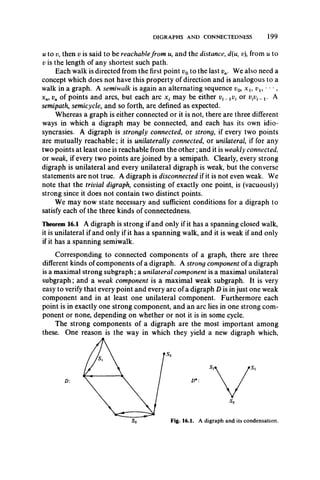
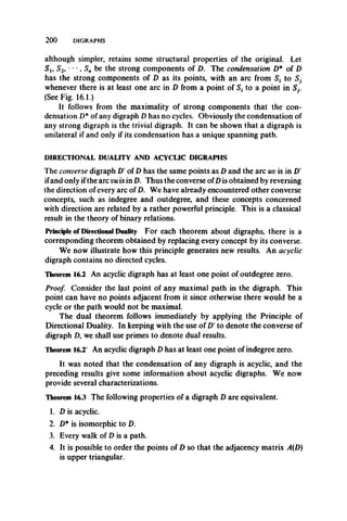
![DIRECTIONAL DUALITY AND ACYCLIC DIGRAPHS 201
Fig. 16.2. An out-tree and the converse in-tree.
Two dual types of acyclic digraphs are of particular interest. A source
in D is a point which can reach all others; a sink is the dual concept. An
out-tree* is a digraph with a source having no semicycles; an in-tree is its
dual, see Fig. 16.2.
Theorem 16.4 A weak digraph is an out-tree if and only if exactly one point
has indegree 0 and all others have indegree 1.
Theorem 16.4' A weak digraph is an in-tree if and only if exactly one point has
outdegree 0 and all others have outdegree 1.
We next consider some digraphs which are closely related to the above.
Afunctional digraph is one in which every point has outdegree 1; a contra-
functional digraph is dual, see Fig. 16.3. The next theorem and its dual
provide structural characterizations.
Theorem 16.5 The following are equivalent for a weak digraph D.
1. D is functional.
2. D has exactly one cycle, the removal of whose arcs results in a digraph
in which each weak component is an in-tree with its sink in the cycle.
3. D has exactly one cycle Z, and the removal of any arc of Z results in an
in-tree.
A point basis of D is a minimal collection of points from which all points
are reachable. Thus, a set S ofpoints ofa digraph D is a point basis ifand only
ifevery point of D is reachable from a point of S and no point of S is reachable
from any other.
Theorem 16.6 Every acyclic digraph has a unique point basis consisting of
all points of indegree 0.
* This is called an “arborescence” by Berge[B12, p. 13].](https://image.slidesharecdn.com/graphtheory-181103155731/85/Graph-theory-212-320.jpg)
![2 0 2 DIGRAPHS
Corollary 16.6(a) Every point basis of a digraph D consists of exactly one
point from each of those strong components in D which form the point
basis of D*.
A I-basis is a minimal collection S of mutually nonadjacent points such
that every point of D is either in S or adjacent from a point of S. Every
digraph has a point basis, but not every digraph has a 1-basis. For example,
no odd cycle has one. A criterion for an arbitrary digraph to have a 1-basis
has not yet been found. The theorem by Richardson [R9] generalizes its
corollary, due to von Neumann and Morgenstern [NM1], and discovered
in their study of game theory.
Theorem 16.7 Every digraph with no odd cycles has a 1-basis.
Corollary 16.7(a) Every acyclic digraph has a 1-basis.
DIGRAPHS AND MATRICES
The adjacency matrix A(D) of a digraph D is the p x p matrix [al7] with
a,j = 1 if vtVj is an arc of Z>, and 0 otherwise. As the example in Fig. 16.4
shows, the row sums of A(D) give the outdegrees of the points of D and the
column sums are the indegrees.
As in the case ofgraphs, the powers of the adjacency matrix A ofa digraph
give information about the number of walks from one point to another.
•«>5
0i 02 •03 04 05 Row sum
01 “0 0 0 0 0 ' 0
02 1 0 1 1 0 3
A(D): v$ 1 0 0 0 0 1
04 0 0 I 0 0 1
05 _0 0 0 0 0_ 0
in sum 2 0 2 1 0
Fig. 16.4. A digraph and its adjacency matrix.](https://image.slidesharecdn.com/graphtheory-181103155731/85/Graph-theory-213-320.jpg)
![DIGRAPHS AND MATRICES 2 0 3
Theorem 16.8 The i, j entry atf of Anis the number of walks of length n from
Vf tO Vj.
We mention briefly three other matrices associated with D, namely the
reachability matrix, the distance matrix, and the detour matrix. In R, the
reachability matrix, is 1 if Vj is reachable from vh and 0 otherwise. The
i, j entry in the distance matrix gives the distance from the point v( to the
point Vj, and is infinity if there is no path from vt to Vj. In the detour matrix,
the z,j entry is the length of any longest path from v{ to vj9 and again is
infinity if there is no such path. These three matrices for the digraph D
of Fig. 16.4 are:
Reachability
Matrix
1 0 0 0 0
1 1 1 1 0
1 0 1 0 0
1 0 1 1 0
0 0 0 0 1
Distance
Matrix
00 00 OO 00
0
00
00
1
0
1
001
00 00
0 oo
00 00 00 00 0
Detour
Matrix
00 00 00 00
000
00
00
2
0
1
1
00 00
0 oo
00 00 00 oo 0
Corollary 16.8(a) The entries of the reachability and distance matrices can
be obtained from the powers of A as follows:
(1) for all I, rH = 1 and dti = 0.
(2) r0 = 1 if and only if for some n, atf > 0.
(3) d(vi9Vj) is the least n (if any) such that aj"* > 0, and is oo otherwise.
There is no efficient method for finding the entries of the detour matrix.
This problem is closely related to several other long-standing algorithmic
questions of graph theory, such as finding spanning cycles and solving the
traveling salesman problem.*
The elementwise product** B x C of two matrices B = [fc0] and C =
[c0] has bijCij as its i, j entry. The reachability matrix can be useful in finding
strong components.
Corollary 16.8(b) Let vt be a point of a digraph D. The strong component of
D containing vt is determined by the entries of 1 in the ith row (or column)
of the matrix R x R T.
The number of spanning in-trees in a given digraph was found by Bott
and Mayberry [BM2] and proved by Tutte [T9]. To give this result, called
* Consider a network N obtained from a strong digraph D by assigning a positive integer
(cost) to every arc of D. The traveling salesman problem asks for an algorithm for finding a
walk in N whereby the salesman can visit each point and return to the starting point while
traversing arcs with a minimum total cost.
** Sometimes called the “ Hadamard product.”](https://image.slidesharecdn.com/graphtheory-181103155731/85/Graph-theory-214-320.jpg)
![2 0 4 DIGRAPHS
l>2 l>3 V2 l?3
Fig. 16.5. Spanning in-trees and out-trees.
the matrix tree theorem for digraphs, we need some other matrices related
to D. Let Afod denote the matrix obtained from —A by replacing the ith
diagonal entry by od(pi). The matrix Afid is defined dually.
Theorem 16.9 For any labeled digraph D, the value of the cofactor of any
entry in the ith row of Mod is the number of spanning in-trees with vt as
sink.
Theorem 16.9' The value of the cofactor of any entry in the yth column of
M id is the number of spanning out-trees with Vj as source.
In accordance with Theorem 16.9, the matrix M ^ of the digraph of
Fig. 16.5 has all cofactors of its entries in the fourth row equal to 3 and the
three spanning in-trees of D with v4 as sink are displayed; the directional
dual, Theorem 16.9', is also illustrated by the second column of M id and the
two spanning out-trees with v2 as source.
An eulerian trail in a digraph D is a closed spanning walk in which each
arc of D occurs exactly once. A digraph is eulerian if it has such a trail. Just
as in Theorem 7.1 for graphs, one can easily show that a weak digraph D is
eulerian if and only if every point of D has equal indegree and outdegree.
We will now state a theorem giving the number ofeulerian trails in an eulerian
digraph. It is sometimes referred to as the BEST theorem after the initials
of de Bruijn, van Aardenne-Ehrenfest, Smith, and Tutte; the first two
[BE1] and the last two [ST1] discovered the theorem independently. It
can be elegantly proved using the matrix tree theorem for digraphs, see
Kasteleyn [K4, p. 76].
Corollary 16.9(a) In an eulerian digraph, the number of eulerian trails is
c - r m - D !
i= 1
where = id^,) and c is the common value of all the cofactors of Afod.](https://image.slidesharecdn.com/graphtheory-181103155731/85/Graph-theory-215-320.jpg)
![TOURNAMENTS 2 0 5
3 - 1 - 1 - 1
2 - 1 0
M^D) =
0 2 - 1
- 1 0 2.
Fig. 16.6. Counting eulerian trails.
Note that for an eulerian digraph D, we have Mod = Afidand all row sums
as well as column sums are zero, so that all cofactors are equal. For the
digraph ip Fig. 16.6, c = 7 and there are 14 eulerian trails. Two of them are
viv2v3v4v2viv3viv4v1and
We havejust given some indication of how matrices are used in the study
of digraphs. On the other hand digraphs can be used to give information
about matrices. Any square matrix M = [mfJ] gives rise to a digraph D,
and also possibly to loops if arc vpj is in D whenever ^ 0. The following
algorithm [H25] sometimes simplifies the determination of the eigenvalues
and the inverse (if it exists) of a matrix Af.
1. Form the digraph D associated with M.
2. Determine the strong components of D.
3. Form the condensation D*.
4. Order the strong components so that the adjacency matrix of D* is
upper triangular.
5. Reorder the points of D by strong components so that its adjacency
matrix A is upper block triangular.
6. Replace each unit entry of A by the entry of M to which it corresponds.
The eigenvalues of M are the eigenvalues of the diagonal blocks of the new
matrix, and the inverse of M can be found from the inverses of these diagonal
blocks.
When M is a sparse matrix,* (or rather has zero entries strategically
located so that there are several strong components), this method can be
quite effective. A generalization to a sometimes more powerful but also more
involved algorithm using bipartite graphs is given by Dulmage and
Mendelsohn [DM2].
TOURNAMENTS
A tournament is an oriented complete graph. All tournaments with two,
three, and four points are shown in Fig. 16.7. The first with three points is
called a transitive triple, the second a cyclic triple.
* In the literature, a sparse matrix has been defined as one with many zeros.](https://image.slidesharecdn.com/graphtheory-181103155731/85/Graph-theory-216-320.jpg)
![2 0 6 DIGRAPHS
Fig. 16.7. Small tournaments.
In a round-robin tournament, a given collection of players or teams
play a game in which the rules of the game do not allow for a draw. Every
pair of players encounter each other and exactly one from each pair emerges
victorious. The players are represented by points and for each pair of
points an arc is drawn from the winner to the loser, resulting in a tournament.
The first theorem on tournaments ever found is due to Redei [R7];
for small tournaments, it can be verified using Fig. 16.7.
Theorem 16.10 Every tournament has a spanning path.
Proof. The proofis by induction on the number ofpoints. Every tournament
with 2, 3, or 4 points has a spanning path, by inspection. Assume the result
is true for all tournaments with n points, and consider a tournament T
with n + 1 points. Let v0 be any point of T. Then T — v0 is a tournament
with n points, so it has a spanning path P., say vx v2 • • • vn. Either arc v0vx
or arc vxv0 is in T. If v0v x is in T, then v0 vx v2 • • • vnis a spanning path of T.
If vxv0 is in T, let v{ be the first point of P for which the arc v0vt is in
T, if any. Then xv0 is in T, so that vx v2 " • 1 v0 r **vnis a spanning
path. If no such point v( exists, then vx v2 • • • vn v0 is a spanning path, in
any case, we have shown that T has a spanning path, completing the proof.
Szele [SI6] extended this result by proving that every tournament has
an odd number of spanning paths. Another type of extension of Redei’s
theorem was provided by Gallai and Milgram [GM1] who showed that
every oriented graph D contains a collection of at most P0{D) point-disjoint
paths which cover V{D).
The next theorem is due to Moser [H M 2]; its corollary was discovered
by Foulkes [F7] and Camion [C l] and is the analogue for strong tourna
ments of the preceding theorem for arbitrary tournaments.
Theorem 16.11 Every strong tournament with p points has a cycle of length n,
for n = 3, 4, • • •, p.
Proof , This proof is also by induction, but on the length of cycles. If a
tournament T is strong, then it must have a cyclic triple. Assume that T](https://image.slidesharecdn.com/graphtheory-181103155731/85/Graph-theory-217-320.jpg)
![TOURNAMENTS 2 0 7
has a cycle Z = vx v2 **- vn vx of length n < p. We will show that it has a
cycle of length n -h i. There are two cases: either there is a point u not
in Z both adjacent to and adjacent from points of Z, or there is no such
point.
CASE 1. Assume there is a point u not in Z and points v and w in Z such
that arcs uv and wu are in T. Without loss of generality, we assume that arc
vxu is in T. Let vt be the first point, going around Z from vu for which arc uvt
is in T. Then i;,_ xu is in T, and vx v2 • • • i>,_jt/1;, • • pn is a cycle of length
n + 1.
CASE 2. There is no such point u as in Case 1. Hence, all points of T which
are not in Z are partitioned into the two subsets U and W, where U is the
set of all points adjacent to every point of Z and W is the set adjacent from
every point of Z. Clearly these sets are disjoint, and neither set is empty
since otherwise T would not be strong. Furthermore, there are points u in
U and w in W such that arc wu is in T. Therefore uvt v2 • • • vn_ xwu is a
cycle of length n + 1 in T.
Hence, there is a cycle of length n + 1, completing the proof.
Corollary 16.11(a) A tournament is strong if and only if it has a spanning
cycle.
Using terminology from round-robin tournaments, we say that the
score of a point in a tournament is its outdegree. The next theorem due to
Landau [LI] was actually discovered during an empirical study of tourna
ments (so-called “pecking orders”) in which the points were hens and the
arcs indicated pecking.
Theorem 16.12 The distance from a point with maximum score to any other
point is 1 or 2.
The number of transitive triples can be given in terms of the scores
of the points; see Harary and Moser [HM2]. As a corollary, one can
readily obtain the well-known formula of Kendall and Smith [KS1], which
has proved useful in statistical analysis. It was generalized from cyclic
triples to larger strong subtournaments by Beineke and Harary [BH4].
Theorem 16.13 The number of transitive triples in a tournament with score
sequence (sl9 s2, • *■, sp) is Z s^s, - l)/2.
Corollary 16.13(a) The maximum number of cyclic triples among all tourna
ments with p points is r 3 _
- - - - - if p is odd,
P - 4p r— —— if p is even.
t(p, 3) =](https://image.slidesharecdn.com/graphtheory-181103155731/85/Graph-theory-218-320.jpg)
![2 0 8 DIGRAPHS
Fig. 16.8. Two pairs of nonreconstructable strong tournaments.
Excursion on Reconstruction of Tournaments
The special case of Ulam’s Conjecture for tournaments has been partially
solved. Just as for graphs, each tournament T with p points determines p
subtournaments 7] = T — vt. We proved* that any nonstrong tournament
with at least five points can be reconstructed. However, the conjecture does
not hold for strong tournaments with p = 5 and 6. This was established
by L. W. Beineke and E. M. Parker, who found that the two pairs of tourna
ments, Fig. 16.8(a, b) and Fig. 16.8(c, d), are counterexamples.
No larger such examples are yet known, and we conjecture that there
are none!
EXERCISES
16.1 A digraph is strictly weak if it is weak but not unilateral; it is strictly unilateral
if it is unilateral but not strong. Let C0 contain all disconnected digraphs, Ct the
strictly weak ones, C2 strictly unilateral, and C3 those which are strong. Then the
maximum and minimum possible number q of arcs among all p point digraphs in
connectedness category Ch i = 0 to 3 is given in the following table:
Category
Minimum Number
of Arcs
Maximum Number
of Arcs
0 0 (p - lXp - 2)
1 P ~ 1 (p - lXp - 2)
2 P ~ 1 (P - I)2
3 P P (P - 1)
(Cartwright and Harary [CHI]
* F. Harary and E. M. Palmer, On the problem of reconstructing a tournament from sub
tournaments, Monatsheftefur Math. 71, 14-23 (1967).](https://image.slidesharecdn.com/graphtheory-181103155731/85/Graph-theory-219-320.jpg)
![EXERCISES 2 0 9
16.2 The cartesian product Dt x D2 of two digraphs has Vl x V2 as its point set,
and (tij, u2) is adjacent to (v1#v2) whenever [«! = Vi and u2adj v2] or [n2 = v2 and
u a4j (This is defined just as for graphs in Chapter 2, except that adjacency is
directed.) When D is in connectedness category C„, we write c{D) = n. Then
c(Dx x D2) = min unless c(Dj) = c(D2) = 2 in which case c{Dl x D2 = 1.
(Harary and Trauth [HT1])
16.3 No strictly weak digraph contains a point whose removal results in a strong
digraph. (Harary and Ross [HR2])
*16.4 There exists a digraph with outdegree sequence (s1} s2, •••, sp), where p — 1 >
Sj > s2 > •• • > spi and indegree sequence (tu t2, • ••, rp) where every tj < p — 1
if and only if 2 s, = 1 r*, and for each integer k < p,
k k p
£ s, ^ £min {fc - 1, tf} + £ min {*, t,}.
i= 1 i=l *=fc+1
(Ryser [R21], Fulkerson [F12])
*16.5 There exists a strong digraph with outdegree and iiidegree sequences as in the
preceding exercise if and only if Z s, = Z th each s, > 0, each t{ > 0, and for each
integer k < p, the following strict inequality holds:
k k p
£ si < £ fi + Z min {k,t,}.
i = l i—1 i=fc+1
(Beineke and Harary [BH1])
16.6 The line digraph L(D) has the arcs of the given digraph D as its points* and x is
adjacent to y in L(D) whenever arcs x, y induce a walk in D. Calculate the number of
points and arcs of L(D) in terms of D. (Harary and Norman [HN4])
16.7 The line digraph L(D) of a weak digraph D is isomorphic to D if and only if D or
D' is functional. (Harary and Norman [HN4])
16.8 If D is disconnected, the assertion in the preceding exercise does not hold.
*16.9 Let S and T be disjoint sets of points of Dand let X(S, T) be the set of all arcs
from S to T. Then D isa line digraph if and onlyif there are no two-point sets S and
T such that |X(S, T) = 3. (Geller and Harary [GH1], Heuchenne [H42])
16.10 The number of eulerian trails of a digraph D equals the number of hamiltonian
cycles of L(D). (Kasteleyn [K3])
16.11 Let Tj consist of one point with 2 directed loops. Let T2 = L(Ti) be the line
digraph (more precisely pseudodigraph) of Tt defined as expected, and recursively let
T„ = L(rn_j). The structures Tn have been called “teleprinter diagrams.” Then the
number of eulerian trails in Tnis
22""1~B- (deBruijn and Ehrenfest [BE1])
*16.12 Every digraph in which id v, od v > p/2 for all points v is hamiltonian.
(Ghouila-Houri [G7])
16.13 Consider those digraphs in which for every point u, the sum £ d(u, r) of the
distances from u is constant. Construct such a digraph which is not point-symmetric.
(Harary [H20])](https://image.slidesharecdn.com/graphtheory-181103155731/85/Graph-theory-220-320.jpg)
![2 1 0 DIGRAPHS
16.14 The complement D and the converse D' both have the same group as D.
16.15 Let A be the adjacency matrix ofthe line digraph ofa complete symmetric digraph.
Then A2 4- A has all entries 1. (Hoffman [H45])
16.16 Two digraphs are cospectral if their adjacency matrices have the same character
istic polynomial. There existjust three different cospectral strong digraphs with 4 points.
(F. Harary, C. King, and R. C. Read)
16.17 The conjunction D = D{ a D2 of two digraphs Dj and D2 has V = Fj x V2
as its point set, and u = (ui9u2) is adjacent to v = (uj, v2) in D whenever w, adj vx in
£>! and u2adj v2 in D2. The adjacency matrix A of the conjunction D = D, a D2 is
the tensor product of the adjacency matrices of Dxand Z)2.
(Harary and Trauth [HT1])
16.18 Let D{ and D2 be digraphs and let d, be the greatest common divisor of the
lengths of all the cycles in Dh i — 1, 2. Then the conjunction Dt a D2 is strong if and
only if Dxand D2are strong and dxand d2are relatively prime. (McAndrew [M7])
16.19 A digraph is called primitive if some power of its adjacency matrix A has all its
entries positive. A digraph is primitive if and only if it is strong and the lengths of its
cycles have greatest common divisor 1. (see Dulmage and Mendelsohn [DM3, p. 204])
*16.20 Let D be a primitive digraph.
a) If n is the smallest integer such that An > 0, then n < (p — l)2 + 1.
(Wielandt [W17])
b) Ifnhas the maximum possible value (p — l)2 + 1, then there exists a permuta
tion matrix P such that PAP~1 has the form [u.J where au = 1 whenever
j — i 4- 1 and apl = 1, but atj = 0 otherwise.
(Dulmage and Mendelsohn [DM3, p. 209])
16.21 An orientation of a graph G is an assignment of a direction to each line of G.
A graph has a strongly connected orientation ifand only if it is connected and bridgeless.
(Robbins [R17])
16.22 Let B be the p x q incidence matrix of an arbitrary orientation D of a given
labeled graph G, so that the entry of B is 4-1 if oriented line xj is incident to point
— 1if Xj is incident from vi9and 0 otherwise. Then the common cofactor of BBTis the
number of spanning trees of G. (Compare the matrix BBTwith M of Chapter 13.)
(Kirchhoff [K7])
16.23 Recall from Chapter 5 that in a graph G, A(w, v) is the minimum number of lines
whose removal separates u and v. Similarly, when u and v are points of a digraph D,
let A(u, v) be the minimum number of arcs whose removal leaves no path from u to v.
For any orientation D of an eulerian graph G, l(u, t;) = l(v, u) = %X(u, v) for every
pair of points. (Nash-Williams [N l])
16.24 Every orientation of an «-chromatic graph G contains a path of length n — 1.
(Gallai [G4])
16.25 The scores s, of a tournament satisfy Z sf = £ (p — 1 —s,)2.](https://image.slidesharecdn.com/graphtheory-181103155731/85/Graph-theory-221-320.jpg)
![EXERCISES 211
16.26 All but two tournaments have a spanning path v2**f pwith a shortcut, the
arc vxvp. The two exceptions are the cyclic triple and tournament of Fig. 16.8(a).
(B. Griinbaum)
16.27 a) The number of cycles of length 4 in any p point tournament is equal to the
number of strong subtournaments with 4 points,
b) The maximum number of strong subtournaments with 4 points in any p
point tournament is t(p, 4) = j(p - 3)r(p, 3). See Corollary 16.13(a).
(Beineke and Harary [BH4])
16.28 A group is isomorphic to the point-group of some tournament if and only if it
has odd order. (Moon [M 14])
16.29 Let T be the point-group and T, the arc-group of a tournament T. Then Tt is
transitive if and only if the pair-group of T is transitive. (Jean [Jl])
16.30 Let t(x) and s(x) be the generating functions for tournaments and strong tourna
ments, respectively. Then
/ >
^ - r n s j
(Moon [M l6, p. 88])
16.31 Consider a sequence of nonnegative integers sx < s2 < •• • < sp.
a) This is the score sequence of some tournament T if and only if
P k
Z si = P(P “ l)/2 and for all k < p, £ > k(k — l)/2.
i i
(Landau [LI])
b) Further, T is strong if and only if for all k < p,
£ S| > k(k - l)/2.
i
(Harary and Moser [HM2])](https://image.slidesharecdn.com/graphtheory-181103155731/85/Graph-theory-222-320.jpg)
![A P P E N D IX 1
GRAPH DIAGRAMS
One picture is worth more
than ten thousand words.
A n o n y m o u s
It is very useful to have diagrams of graphs available for the accumulation
of data leading to conjectures. Graphs with fewer than 6 points are easily
drawn. The diagrams of 6 point graphs which are presented here were
produced by D. W. Crowe, who also was apparently the first to draw all
7 point graphs. In listing the diagrams, no attempt was made to settle the
problem of assigning a canonical ordering to the various graphs with p
points and q lines. However an index n is assigned to each graph G, with the
same index going to the complementary graph G. Thus the graph Gpqn is
the nth (p, q) graph, and is identified to the right of its diagram by the
number n ; furthermore Gpqn = GPt(p)-qn. The (4, 3) and (5, 5) graphs
are of course exceptions to this rule.
As a supplement to tables of this kind, B. R. Heap developed a program
on the computer at the National Physical Laboratory in Middlesex which
has produced one card for each graph with 7 points and is in the process
of producing graphical cards for p = 8. It was found most convenient to
code the graphs in adjacency matrix form. The existence of such lists has
already proved valuable to investigators using computer methods.
For convenience we present here a table displaying the number of
graphs with a given number of points and lines, up through 9 points (cf.
Riordan [R15, p. 146]). The entries were obtained using Polya’s formula
(15.47).
213](https://image.slidesharecdn.com/graphtheory-181103155731/85/Graph-theory-224-320.jpg)

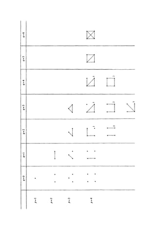
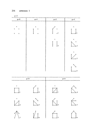
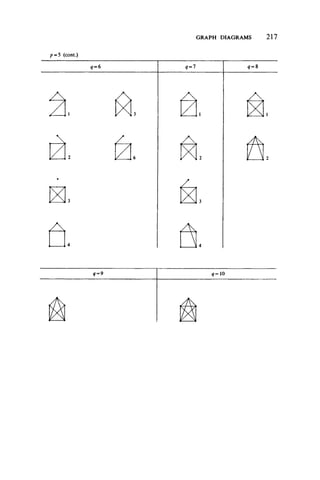
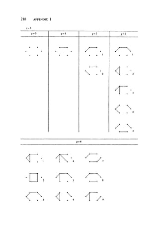
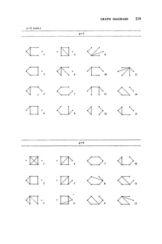
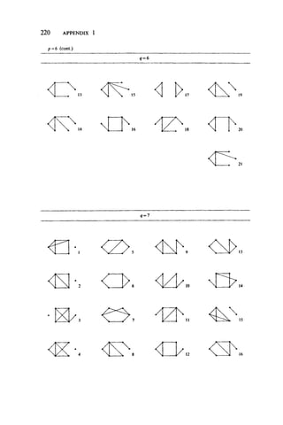
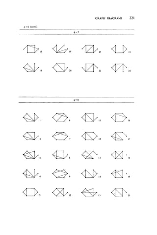
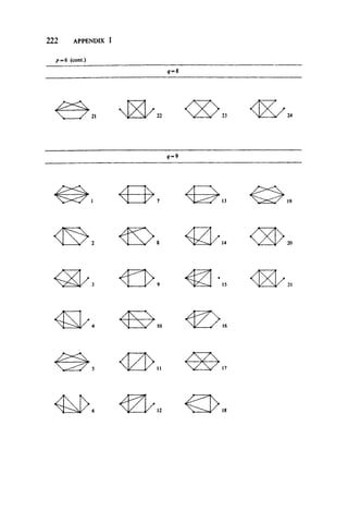
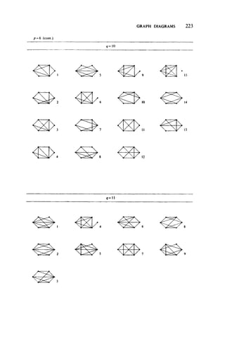
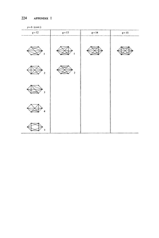
![A P P E N D IX 2
DIGRAPH DIAGRAMS
The hero jumped on his horse
and rode off in all directions.
S. L e a c o c k
The digraphs with at most 4 points are listed here according to the number
of points and arcs. Indices are assigned to each one in such a way that
complements receive the same index, except of course within the (3, 3) and
(4, 6) digraphs. The diagrams only go through p = 4 because to include
those for p = 5 would require another book almost the size of the present
volume. The following table due to Oberschelp [O l] gives the number of
digraphs with p points, p < 8. The entries may be computed using
equations (15.31, 15.32).
Table A2
THE NUMBER
OF DIGRAPHS
WITH p < 8 POINTS
p dP
1 1
2 3
3 16
4 218
5 9 608
6 1 540 944
7 882 033 440
8 1 793 359 192 848
225](https://image.slidesharecdn.com/graphtheory-181103155731/85/Graph-theory-236-320.jpg)
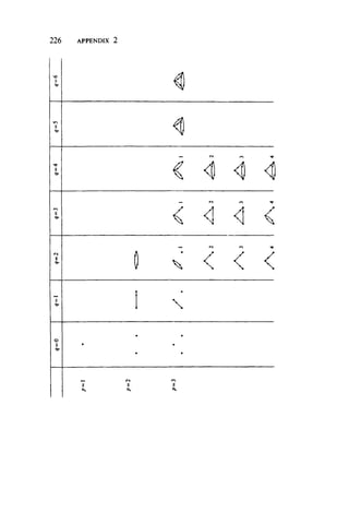
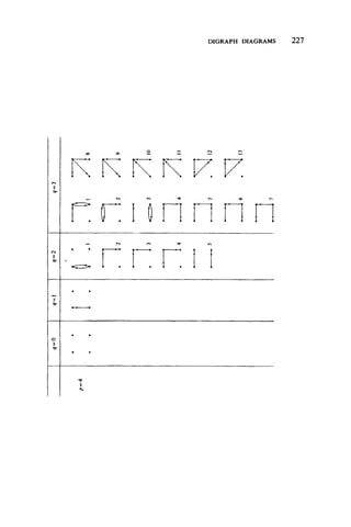
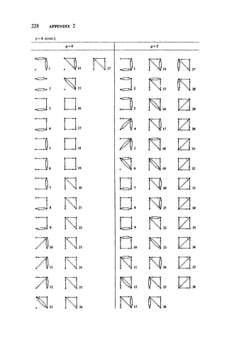
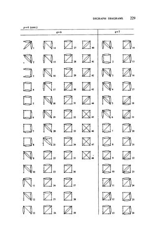
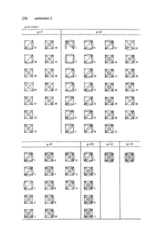
![A P P E N D IX 3
TREE DIAGRAMS
You can’t see the forest for the trees.
A n o n y m o u s
The diagrams of all the trees with p < 12 points were developed by Prins
and appear as an appendix in his doctoral dissertation [P8]. We present
here only those diagrams for p < 10, which are also given in [HP21]. The
ordering of trees with a given number of points is somewhat arbitrary, but in
general they are listed by increasing number of points of degree greater than
2. The following table presents the number of trees and rooted trees with p
points for p < 26 (cf. Riordan [R15, p. 138]) and the number of identity
trees and homeomorphically irreducible trees for p < 12 (cf. [HP20]).
These numbers were obtained using formulas (15.41), (15.35), (15.51 and
15.52), and (15.47, 15.48, and 15.49) respectively.
231](https://image.slidesharecdn.com/graphtheory-181103155731/85/Graph-theory-242-320.jpg)
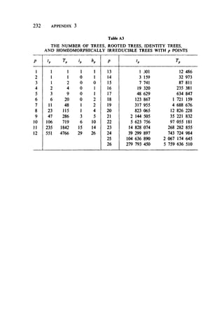
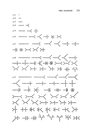
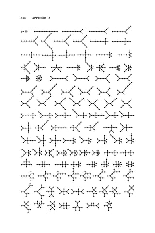

![BIBLIOGRAPHY
And thick and fast
They came at last,
And more and more and more.
L. C a r r o l l
The references listed below are intended to be those and only those which have been
cited in the text. It should be noted, however, that this list is considerably more selective
than the exceedingly comprehensive bibliography of graph theory and its applications
compiled by Turner [T5]. For the convenience of the reader, each item in this bibliog
raphy is followed by one or more numbers in square bracketswhich indicate the pages
where the item is mentioned, following the useful innovationof Griinbaum[G10]. In
accordance with the procedure in Mathematical Reviews, all books are starred.!
Anderson, S. S.
[AH1] (with F. Harary), Trees and unicyclic graphs. Math. Teacher 60 (1967),
345-348. [42]
Babler, F.
[Bl] Uber eine spezielle Klasse Euler’scher Graphen. Comment. Math. Helv.
27 (1953), 81-100. [69]
Balaban, A. T.
[B2] Valence-isomerism of cyclopolyenes. Rev. Roumaine Chim. 11 (1966),
1097-1116. [62]
Ball, W. W. R.
* [BC1] (with H. S. M. Coxeter), Mathematical Recreations and Essays.
Macmillan, New York, 1947. [4]
Barnette, D.
[B3] Trees in polyhedral graphs. Canad. J. Math. 18 (1966), 731-736. [124]
See also p. 68.
f One publisher advertised a trigonometry text saying, “This book was starred in Math. Reviews.”
237](https://image.slidesharecdn.com/graphtheory-181103155731/85/Graph-theory-248-320.jpg)
![238 BIBLIOGRAPHY
Battle, J.
[BHK1] (with F. Harary and Y. Kodama), Every planar graph with nine points
has a nonplanar complement. Bull. Amer. Math. Soc. 68 (1962),
569-571. [108]
[BHKY1] (with F. Harary, Y. Kodama, J. W. T. Youngs), Additivity of the genus of
a graph. Bull. Amer. Math. Soc. 68 (1962), 565-568. [119]
Behzad, M.
[B4] A criterion for the planarity of a total graph. Proc. Cambridge Philos.
Soc. 63 (1967), 679-681. [71, 82, 124]
[BC2] (with G. Chartrand), Total graphs and traversability. Proc. Edinburgh
Math. Soc. 15 (1966), 117-120. [83]
[BC3] (with G. Chartrand), No graph is perfect. Amer. Math. Monthly 74
(1967), 962-963. [62]
[BCC1] (with G. Chartrand and J. Cooper), The colour numbers of complete
graphs. J. London Math. Soc. 42 (1967), 226-228. [149]
[BCN1] (with G. Chartrand and E. A. Nordhaus), Triangles in line-graphs and
total graphs. Indian J. Math, (to appear). [83]
[BR1] (with H. Radjavi), The line analog of Ramsey numbers. Israel J. Math.
5(1967), 93-96. [82]
Beineke, L. W.
[B5] Decompositions of complete graphs into forests. Magyar Tud. Akad.
Mat. Kutato Int. Kozl. 9 (1964), 589-594. [91]
[B6] The decomposition ofcomplete graphs into planar subgraphs. Chapter 4
in Graph Theory and Theoretical Physics (F. Harary, ed.) Academic
Press, London, 1967, pp. 139-154. [120]
[B7] Complete bipartite graphs: decomposition into planar subgraphs.
Chapter 7 in A Seminar in Graph Theory (F. Harary, ed.) Holt, Rinehart
and Winston, New York, 1967, pp. 42-53. [120]
[B8] Derived graphs and digraphs. Beitrdge zur Graphentheorie (H. Sachs,
H. Voss, and H. Walther, eds.) Teubner, Leipzig, 1968, pp. 17-33.
[71,74]
[BG1] (with R. K. Guy), The coarseness of Kmn. Canad. J. Math, (to appear).
[121, 125]
[BH1] (with F. Harary), Local restrictions for various classes of directed
graphs. J. London Math. Soc. 40 (1965), 87-95. [209]
[BH2] (with F. Harary), Inequalities involving the genus of a graph and its
thickness. Proc. Glasgow Math. Assoc. 7 (1965), 19-21. [118, 125]
[BH3] (with F. Harary), The genus of the n-cube. Canad. J. Math. 17 (1965),
494-496. [119]
[BH4] (with F. Harary), The maximum number of strongly connected sub-
tournaments. Canad. Math. Bull. 8 (1965), 491-498. [207, 211]
[BH5] (with F. Harary), The thickness of the complete graph. Canad. J. Math.
17(1965X 850-859. [120]
[BH6] (with F. HararyX The connectivity function of a graph. Mathematika
14(1967), 197-202. [45,51]
[BHM1] (with F. Harary and J. W. MoonX On the thickness of the complete
bipartite graph. Proc. Cambridge Philos. Soc. 60 (1964), 1-5. [120]](https://image.slidesharecdn.com/graphtheory-181103155731/85/Graph-theory-249-320.jpg)
![BIBLIOGRAPHY 2 3 9
[BHP1]
[BM1]
[BP1]
[BP2]
Benzer, S.
[B9]
Berge, C.
[BIO]
(with F. Harary and M. D. Plummer), On the critical lines of a graph.
Pacific J. Math. 22 (1967), 205-212. [98]
(with J. W. Moon), The number of labelled A>trees. Proof Techniques
in Graph Theory (F. Harary, ed.) Academic Press, New York, 1969.
[195]
(with R. E. Pippert) The enumeration of labelled /c-dimensional trees.
J. Combinatorial Theory (to appear). [195]
(with M. D. Plummer), On the 1-factors of a nonseparable graph.
J. Combinatorial Theory 2 (1967), 285-289. [85, 92]
See also [GB1].
On the topology of the genetic fine structure. Proc. Nat. Acad. Sci. USA
45 (1959), 1607-1620. [20]
* [BH]
* [B12]
[BG2]
Two theorems in graph theory. Proc. Nat. Acad. Sci. USA 43 (1957),
842-844. [96]
Theorie des Graphes et ses Applications. Dunod, Paris, 1958. [44]
The Theory of Graphs and its Applications. Methuen, London, 1962.
[21, 97, 100, 128, 201]
(with A. Ghouila-Houri), Programming, Games, and Transportation
Networks. Methuen, London, 1965. [7]
Binet, J. P. M. See p. 153.
Birkhoff, G.
* [B13] Lattice Theory. Amer. Math. Soc. Colloq. Publ., Vol. 25, Third Edition,
Providence, 1967. [54]
Birkhoflf, G. D.
[BL1] (with D. Lewis), Chromatic polynomials. Trans. Amer. Math. Soc. 60
(1946), 355-451. [145]
Boland, J.
[BL2]
Bollobas, B.
[B14]
Bondy, J. A.
[815]
(with C. Lekkerkerker), Representation of a finite graph by a set of
intervals on the real line. Fund. Math. 51 (1962), 45-64. [21]
On graphs with at most three independent paths connecting any two
vertices. Studia Sci. Math. Hungar. 1 (1966), 137-140. [55, 56]
On Kelly’s congruence theorem for trees. Proc. Cambridge Philos. Soc.
65(1969), 1-11. [41]
See also p. 149.
Bosak, J. See p. 68.
Bott, R.
[BM2] (with J. P. Mayberry), Matrices and trees. Economic activity analysis.
(O. Morgenstern, ed.) New York, Wiley, 391-400. [203]
Brooks, R. L.
[B16] On colouring the nodes of a network. Proc. Cambridge Philos. Soc. 37
(1941) 194-197. [128]](https://image.slidesharecdn.com/graphtheory-181103155731/85/Graph-theory-250-320.jpg)
![2 4 0 BIBLIOGRAPHY
[BSST1]
Brualdi, R. A.
[B17]
deBruijn, N. G.
[B18]
[B19]
[BE1]
(with C. A. B. Smith, A. H. Stone, and W. T. Tutte), The dissection of
rectangles into squares. Duke Math.J. 7 (1940), 312-340. [158]
See also p. 123.
Kronecker products of fully indecomposable matrices and of ultrastrong
digraphs, J. Combinatorial Theory 2 (1967), 135-139. [21]
Generalization of Polya’s fundamental theorem in enumeration com
binatorial analysis. Indagationes Math. 21 (1959), 59-69. [191]
Polya’s theory of counting. Applied Combinatorial Mathematics
(E. F. Beckenbach, ed.) Wiley, New York, 1964, pp. 144-184. [191]
(with T. van Aardenne-Ehrenfest), Circuits and trees in oriented graphs.
Simon Stevin 28 (1951), 203-217. [195, 204, 209]
Burnside, W.
* [B20]
Cameron, J.
Camion, P.
[Cl]
Carlitz, L.
[CRl]
Cartwright D.
[CHI]
Theory of Groups of Finite Order(second edition)Cambridge Univ.
Press, Cambridge, 1911. [ 180]
See p. 25.
Chemie et circuits hamiltoniens des graphes complets.C.R. Acad. Sci.
Paris 249 (1959), 2151-2152. [206]
[CH2]
Cauchy, A. L.
Cayley, A.
[C2]
[C3]
[C4]
[C5]
[C6]
Chang, L. C.
[C7]
(with J. Riordan), The number of labelled two-terminal series-parallel
networks. Duke Math. J. 23 (1955), 435-445. [195]
(with F. Harary), The number of lines in a digraph of each connectedness
category. SIAM Review 3 (1961), 309-314. [208]
(with F. Harary), On colorings of signed graphs. Elem. Math. 23
(1968), 85-89. [138, 149]
See also [HNC1].
See p. 153.
On the theory of the analytical forms called trees. Philos. Mag. 13 (1857),
19-30. Mathematical Papers, Cambridge 3 (1891), 242-246. [3, 187]
On the mathematical theory of isomers. Philos. Mag. 67 (1874), 444-446.
Mathematical Papers, Cambridge 9 (1895), 202-204; and 9 (1895),
427-460. [3]
The theory of groups, graphical representation. Mathematical Papers,
Cambridge 10 (1895), 26-28. [168]
On the analytical forms called trees. Amer. Math. J. 4 (1881), 266-268.
Mathematical Papers, Cambridge 11 (1896), 365-367. [188]
A theorem on trees. Quart. J. Math. 23 (1889), 376-378. Mathematical
Papers,, Cambridge 13 (1897), 26-28. [179, 195]
The uniqueness and nonuniqueness of the triangular association scheme.
Sci. Record 3 (1959), 604-613. [78]](https://image.slidesharecdn.com/graphtheory-181103155731/85/Graph-theory-251-320.jpg)
![BIBLIOGRAPHY 241
Chartrand, G.
[C8] A graph-theoretic approach to a communications problem. J. SIAM
Appl. Math. 14 (1966), 778-781. [44]
[C9] On Hamiltonian line graphs. Trans. Amer. Math. Soc. (to appear).
[81]
[CGI] (with D. Geller), Uniquely colorable planar graphs. J. Combinatorial
Theory (to appear). [138, 140, 149]
[CGH1] (with D. Geller and S. Hedetniemi), A generalization of the chromatic
number. Proc. Cambridge Philos. Soc. 64 (1968), 265-211. [149]
[CGH2] (with D. Geller and S. Hedetniemi), Graphs with forbidden subgraphs.
J. Combinatorial Theory (to appear). [25, 100, 124]
[CH3] (with F. Harary), Planar permutation graphs. Ann. Inst. Henri Poincare
Sec. B 3 (1967), 433-438. [107, 175, 177]
[CH4] (with F. Harary), Graphs with prescribed connectivities. Theory of
Graphs (P. Erdos and G. Katona, eds.) Akademiai Kiado, Budapest,
1968,61-63. [44]
[CKK1] (with S. F. Kapoor and H. V. Kronk), The Hamiltonian hierarchy.
(to appear). [70]
[CKL1] (with A. Kaugars and D. R. Lick) Critically n-connected graphs.
Proc. Amer. Math. Soc. (submitted). [56]
[CK1] (with H. V. Kronk), Randomly traceable graphs. J. SIAM Appl. Math.
(to appear). [70]
[CS1] (with M. J. Stewart) The connectivity of line-graphs. Math. Ann.
(submitted). [83]
See also [BC2], [BC3], [BCC1], [BCN1], [KC1], and p. 77.
Cooper, J. See [BCC1].
Courant, R.
* [CR1] (with H. E. Robbins) What is Mathematics? Oxford U. Press, London,
1941. [117]
Coxeter, H. S. M.
[CIO] Self-dual configurations and regular graphs. Bull. Amer. Math. Soc.
56 (1950), 413-455. [175]
See also [BC1].
Crowe, D. W. See p. 213.
Danzer, L.
[DK.1] (with V. Klee) Lengths of snakes in boxes. J. Combinatorial Theory
2 (1967), 258-265. [25]
Dauber, E. See p. 172.
Davis, R. L.
[D l]
[D2]
The number of structures of finite relations. Proc. Amer. Math. Soc. 4
(1953), 486-495. [195]
Structures of dominance relations. Bull. Math. Biophys. 16 (1954),
131-140. [195]](https://image.slidesharecdn.com/graphtheory-181103155731/85/Graph-theory-252-320.jpg)
![2 4 2 BIBLIOGRAPHY
Descartes, B.
[D3] Solution to advanced problem no. 4526. Amer. Math. Monthly 61
(1954), 352. [128]
Dilworth, R. P.
[D4] A decomposition theorem for partially ordered sets. Ann. Math. 51
(1950), 161-166. [54]
Dirac, G. A.
[D5] A property of 4-chromatic graphs and some remarks on critical graphs.
J. London Math. Soc. 27 (1952), 85-92. [135, 141]
[D6] Some theorems on abstract graphs. Proc. London Math. Soc., Ser. 3, 2
(1952), 69-81. [68, 142]
[D7] The structure of k-chromatic graphs. Fund. Math. 40 (1953), 42-55.
[128, 142]
[D8] In abstrakten Graphen verhandene vollstandige 4-Graphen und ihre
Unterteilungen. Math. Nachr. 22 (I960), 61-85. [45,149]
[D9] Generalisations du theoreme de Menger. C.R. Acad. Sci. Paris 250
(1960), 4252-4253. [50]
[DIO] Short proof of Menger’s graph theorem. Mathematika 13 (1966),
42-44. [47]
[D ll] On the structure of k-chromatic graphs. Proc. Cambridge Philos. Soc.
63 (1967), 683-691. [149]
[DS1] (with S. Schuster), A theorem of Kuratowski. Nederl. Akad. Wetensch.
Proc. Ser. A 57 (1954), 343-348. [108]
Dulmage, A. L.
[DM 1] (with N. S. Mendelsohn), Coverings of bipartite graphs. Canad. J. Math.
10(1958), 517-534. [98,99]
[DM2] (with N. S. Mendelsohn), On the inversion of sparse matrices. Math.
Comp. 16 (1962), 494-496. [205]
[DM3] (with N. S. Mendelsohn), Graphs and matrices. Chapter 6 in Graph
Theory and Theoretical Physics (F. Harary, ed.) Academic Press, London,
1967, pp. 167-229. [210]
Edmonds, J.
[E l] Existence of k-edge connected ordinary graphs with prescribed degrees.
J. Res. Nat. Bur. Stand., Sect.B 68 (1964), 73-74. [63]
Ehrenfest, T. van Aardenne-. See [BE1].
Elias, P.
[EFS1] (with A. Feinstein and C. E. Shannon), A note on the maximum flow
through a network. IRE Trans. Inform. Theory, IT-2, (1956), 117-119.
[49]
Erdos, P
[E2] Graph theory and probability II. Canad. J. Math. 13 (1961), 346-352.
[128]
[E3] Extremal problems in graph theory. Chapter 8 of A Seminar on Graph](https://image.slidesharecdn.com/graphtheory-181103155731/85/Graph-theory-253-320.jpg)
![BIBLIOGRAPHY 2 4 3
Theory (F. Harary, ed.) Holt, Rinehart and Winston, New York, 1967,
pp. 54-59. [17, 18, 25]
[E4] Applications of probabilistic methods to graph theory. Chapter 9 in
A Seminar on Graph Theory (F. Harary, ed.) Holt, Rinehart and Winston,
New York, 1967, pp. 60-64. [24]
[EG1] (with T. Gallai) Graphs with prescribed degrees of vertices (Hungarian).
Mat. Lapok II (1960), 264-274. [58, 59]
[EGP1] (with A. Goodman and L. Posa) The representation of a graph by set
intersections. Canad. J. Math. 18 (1966), 106-112. [20]
[EH1] (with A. Hajnal) On chromatic numbers of graphs and set-systems.
Acta Math. Acad. Sci. Hungar. 17 (1966), 61-99. [148]
[ER1] (with A. Renyi) Asymmetric graphs. Acta Math. Acad. Sci. Hungar. 14
(1963), 295-315. [17]
[ESI] (with G. Szekeres) A combinatorial problem in geometry. Compositio
Math. 2 (1935), 463-470. [16]
See also p. 121.
Euler, L.
[E5] Solutio problematis ad geometriam situs pertinentis. Comment. Acade-
miae Sci. I. Petropolitanae 8 (1736) 128-140. Opera Omnia Series 1-7
(1766), 1-10. [2]
The Konigsberg bridges. Sci. Amer. 189 (1953) 66-70. [14]
See also p. 64 and 103.
(with F. Harary and M. S. Lynn) On the computer enumeration of finite
topologies. Comm. Assoc. Comp. Mach. 10 (1967), 295-298. [195]
See [AFPR1].
[E6]
Evans, J. W.
[EHL1]
Fagen, R. E.
Fary, I.
[Fl]
Feinstein, A.
Feller, W.
* [F2]
Feynmann, R.
[F3]
Finck, H. J.
[F4]
[FS1]
Folkman, J.
[F5]
On straight line representation of planar graphs. Acta Sci. Math.
Szeged. 11 (1948) 229-233. [106]
See [EFS1].
An Introduction to Probability Theory and its Applications, Vol. 1,
(2nd ed.) Wiley, New York, 1957. [6]
P.
Space-time approaches to quantum electrodynamics. Physical Review
76 (1949) 769-789. [6]
Uber die chromatischen Zahlen eines Graphen und Seines Komplements,
I and II. Wiss. Z. T. H. Ilmenau 12 (1966), 243-251. [148]
(with H. Sachs), Uber eine von H. S. Wilf angegebene Schranke fur
die chromatische Zahl endlicher Graphen. Math. Nachr. 39 (1969),
373-386. [132]
Regular line-symmetric graphs. J. Combinatorial Theory (to appear).
[173]](https://image.slidesharecdn.com/graphtheory-181103155731/85/Graph-theory-254-320.jpg)
![2 4 4 BIBLIOGRAPHY
Ford, G. W.
[FNU1] (with R. Z. Norman and G. E. Uhlenbeck), Combinatorial problems in
the theory of graphs, II. Proc. Nat. Acad. Sci. USA 42 (1956), 203-208.
[195]
Ford, L. R.
[FF1] (with D. R. Fulkerson), Maximal flow through a network, Canad. J.
Math. 8 (1956), 399-404. [49]
* [FF2] (with D. R. Fulkerson), Flows in Networks. Princeton University Press,
Princeton, 1962. [7, 52]
Foster, R. M.
[F6] Geometrical circuits of electrical networks. Trans. Amer. Inst. Elec.
Engrs. 51 (1932), 309-317. [171]
Foulkes, J. D.
[F7] Directed graphs and assembly schedules. Proc. Symp. Appl. Math.,
Amer. Math. Soc. 10 (1960), 281-289. [206]
Frucht, R.
[F8] Herstellung von Graphen mit vorgegebener abstrakten Gruppe.
Compositio Math. 6 (1938), 239-250. [168]
[F9] Graphs of degree three with a given abstract group. Canad. J. Math. 1
(1949), 365-378. [170]
[F10] On the groups of repeated graphs. Bull. Amer. Math. Soc. 55 (1949),
418-420. [165]
[FI 1] A one-regular graph of degree three. Canad. J. Math. 4 (1952), 240-247.
[175]
[FH1] (with F. HararyX On the corona of two graphs. Aequationes Math.
(to appear). [167]
See also p. 168.
Fulkerson, D. R.
[FI2] Zero-one matrices with zero trace. Pacific J. Math. 10 (I960), 831-836.
[209]
[FI3] Networks, frames, and blocking systems. Mathematics of the Decision
Sciences. Vol. II, Lectures in Applied Mathematics, (G. B. Dantzig
and A. F. Scott, eds.) 303-334. [52]
See also [FF1], and [FF2].
Gaddum, J. W. See [NG1].
Gallai, T.
[GI] On factorisation of graphs. Acta Math. Acad. Sci. Hungar. 1 (1950),
133-153. [85]
[G2] Uber extreme Punkt- und Kantenmengen. Ann. Univ. Sci. Budapest,
Eotvos Sect. Math. 2 (1959), 133-138. [95]
[G3] Elementare relationen beziiglich der glieder und trennenden punkte von
graphen. Magyar Tud. Akad. Mat. Kutato Int. Kozl. 9 (1964), 235-236.
[31, 36]
[G4] On directed paths and circuits. Theory of Graphs (P. Erdos and G.
Katona, eds.) Akademiai Kiado, Budapest, 1968. Also Academic Press,
New York, 1968, pp. 115-119. [149, 210]](https://image.slidesharecdn.com/graphtheory-181103155731/85/Graph-theory-255-320.jpg)
![BIBLIOGRAPHY 245
[GM1] (with A. N. Milgram) Verallgemeinerung eines graphen theoretischen
Satzes von Redei, Acta Scient. Math. 21 (1960), 181-186. [206]
See also [EG1].
Gaudin, T.
[GHR1] (with J. C. Herz and P. Rossi) Solution du probleme no. 29. Rev. Franc.
Rech. Oper. 8 (1964), 214-218. [70]
Geller, D. P.
[G5] Outerplanar graphs, (to appear). [108]
[GH1] (with F. Harary), Arrow diagrams are line digraphs. J. SIAM Appl
Math. 16 (1968), 1141-1145. [209]
See also [CGI], [CGH1], [CGH2], and p. 83.
Gerencser, L.
[G6] On coloring problems (Hungarian). Mat. Lapok 16 (1965) 274-277.
[101]
Gewirtz, A.
[GQ1] (with L. V. Quintas) Connected extremal edge graphs having symmetric
automorphism group. Recent Progress in Combinatorics (W. T. Tutte,
ed.) Academic Press, New York, 1969. [176]
Ghouila-Houri, A.
[G7] Une condition suffisante d’existence d’un circuit hamiltonien. C. R.
Acad. Sci. Paris 251 (1960), 495-497. [209]
See also [BG2].
Gilbert, E. N.
[GR1] (with J. Riordan) Symmetry types of periodic sequences. IllinoisJ. Math.
5 (1961), 657-665. [195]
Gilmore, P.
[GH2] (with A. J. Hoffman) A characterization of comparability graphs and
interval graphs. Canad. J. Math. 16 (1964) 539-548. [21]
Goodman, A. See [EGP1].
Graver, J. E.
[GY1] (with J. Yackel) Some graph theoretic results associated with Ramsey’s
theorem. J. Combinatorial Theory 4 (1968), 125-175. [16]
Grossman, J. W. See [HG1].
Grotzsch, H.
[G8] Ein Dreifarbensatz fur dreikreisfreie Netze auf der Kugel. Wiss. Z.
Martin-Luther Univ. Halle-Wittenberg. Math. Naturwiss. Reihe 8 (1958),
109-120. [131]
Griinbaum, B.
*[G9] Grotzsch’s theorem on 3-colorings. Michigan Math. J. 10 (1963),
303-310. [131]
[G10] Convex Polytopes, Wiley (Interscience) New York, 1967.
[68, 117, 235]
See also p. 211.](https://image.slidesharecdn.com/graphtheory-181103155731/85/Graph-theory-256-320.jpg)
![2 4 6 BIBLIOGRAPHY
Gupta, R. P.
[G il]
Guy, R. K.
* [G12]
[GB1]
Independence and covering numbers of line graphs and total graphs.
Proof Techniques in Graph Theory (F. Harary, ed.) Academic Press,
New York, 1969. [97]
The decline and fall of Zarankiewicz’s theorem. Proof Techniques in
Graph Theory (F. Harary, ed.) Academic Press, New York, 1969. [122]
(with L. W. Beineke), The coarseness of the complete graph. Canad. J.
Math. 20 (1966), 888-894. [121]
See also [BG1].
Hadwiger, H.
[HI]
Hajnal, A.
Hajos, G.
[H2]
[H3]
Hakimi, S.
[H4]
Halin, R.
[H5]
Hall, D. W.
[H6]
Hall, M.
* [H7]
Hall, P.
[H8]
Hamelink, R. C.
Uber eine Klassifikation der Streckenkomplexe.
forsch. Ges. Zurich 88 (1943), 133-142.
See [EH1].
Vierteljschr. Natur-
[135]
Uber eine Art von Graphen. Internat. Math. Nachr. 2 (1957), 65. [20]
Uber eine Konstruktion nicht n-farbbarer Graphen. Wiss. Z. Martin
Luther Univ. Halle-Wittenberg Math.-Natur. Reihe. 10(1961), 116-117.
[143]
On the realizability of a set of integers as degrees of the vertices of a
graph. J. SIAM Appl. Math. 10 (1962), 496-506. [58, 62, 63]
A theorem on w-connected graphs. J. Combinatorial Theory (to appear).
[56]
A n o te o n p r im itiv e s k e w c u r v e s .
935-937.
Bull. Amer. Math. Soc. 49 (1943),
[123]
Combinatorial Theory, Blaisdell, Waltham, 1967. [16, 56]
[H9]
Harary, F.
[H10]
[H ll]
[H12]
[H I 3]
On representations of subsets. J. London Math. Soc. 10 (1935), 26-30.
[53]
Combinatorial Theory
[20]
A partial characterization of clique graphs,
(to appear).
On the notion of balance of a signed graph. Mich. Math. J. 2 (1953),
143-146. [195]
The number of linear, directed, rooted, and connected graphs. Trans.
Amer. Math. Soc. 78 (1955), 445-463. [185, 186, 195]
Note on the Polya and Otter formulas for enumerating trees. Mich.
Math. J. 3 (1956), 109-112. [189]
On the number of dissimilar line-subgraphs of a given graph. Pacific J.
Math. 6 (1956), 57-64. [195]](https://image.slidesharecdn.com/graphtheory-181103155731/85/Graph-theory-257-320.jpg)
![BIBLIOGRAPHY 247
[HI 5]
[H16]
[H17]
[HI8]
[HI 9]
[H20]
[H21]
[H22]
[H23]
[H24]
[H25]
[H26]
[H27]
[H28]
[H29]
[H30]
[H31]
[H32]
[H33]
[HH1]
[H14]
[HHP1]
The number of dissimilar supergraphs of a linear graph. Pacific J. Math.
7 (1957), 903-911. [195]
Structural duality. Behavioral Sci. 2 (1957), 255-265. [30]
The number of oriented graphs. Mich. Math. J. 4 (1957), 221-224.
[195]
On arbitrarily traceable graphs and directed graphs. Scripta Math. 23
(1957), 37-41. [69]
On the number of bicolored graphs. Pacific J. Math. 8 (1958), 743-755.
[163, 177]
On the number of dissimilar graphs between a given graph-subgraph
pair. Canad. J. Math. 10 (1958), 513-516. [195]
Status and contrastatus. Sociometry 22 (1959), 23-43. [209]
On the group of the composition of two graphs. Duke Math. J. 26
(1959), 29-34. [21, 166]
An elementary theorem on graphs. Amer. Math. Monthly 66 (1959),
405-407. [31]
The number of functional digraphs. Math. Ann. 138 (1959), 203-210.
[195]
Unsolved problems in the enumeration of graphs. Publ. Math. Inst.
Hung. Acad. Sci. 5 (1960), 63-95. [192]
A graph theoretic approach to matrix inversion by partitioning. Numer.
Math. 4 (1962), 128-135. [205]
The maximum connectivity of a graph. Proc. Nat. Acad. Sci. USA 48
(1962), 1142-1146. [44]
The determinant of the adjacency matrix of a graph. SIAM Review 4
(1962), 202-210. [151]
A characterization of block-graphs. Canad. Math. Bull. 6 (1963), 1-6.
[30]
On the reconstruction of a graph from a collection of subgraphs. Theory
of Graphs and its Applications (M. Fiedler, ed.). Prague, 1964, 47-52;
reprinted, Academic Press, New York, 1964. [12, 41]
Combinatorial problems in graphical enumeration. Applied Combina
torial Mathematics (E. F. Beckenbach, ed.) Wiley, New York, 1964,
pp. 185-220. [192]
Applications of Polya’s theorem to permutation groups. Chapter 5 in
A Seminar on Graph Theory (F. Harary, ed.) Holt, Rinehart and Winston,
New York, 1967, pp. 25-33. [183, 184, 185, 195]
Graphical enumeration problems. Chapter 1 in Graph Theory and
Theoretical Physics (F. Harary, ed.) Academic Press, London, 1967,
pp. 1-41. [192, 194]
Variations on a theorem by Menger. J. SIAM Appl. Math, (to appear).
[55]
(with S. Hedetniemi), The achromatic number of a graph. J. Combina
torial Theory (to appear). [128, 144]
(with S. Hedetniemi and G. Prins), An interpolation theorem for graphical
homomorphisms. Port. Math, (to appear). [143, 144, 149]](https://image.slidesharecdn.com/graphtheory-181103155731/85/Graph-theory-258-320.jpg)
![248 BIBLIOGRAPHY
[HHR1]
[HKT1]
[HK1]
[HM1]
[HM2]
[HMR1]
[HN1]
[HN2]
[HN3]
[HN4]
* [HNC1]
[HP1]
[HP2]
[HP3]
[HP4]
[HP5]
[HP6]
[HP7]
[HP8]
[HP9]
[HP10]
[HP11]
[HP12]
(with S. T. Hedetniemi and R. W. Robinson), Uniquely colorable graphs.
J. Combinatorial Theory (to appear). [139, 149]
(with R. M. Karp and W. T. Tutte), A criterion for planarity of the
square of a graph. J. Combinatorial Theory 2 (1967), 395-405. [124]
(with Y. Kodama), On the genus of an n-connected graph. Fund. Math.
54 (1964), 7-13. [47,119]
(with B. Manvel), On the number of cycles in a graph. Math, casopis
(to appear). [25,158]
(with L. Moser), The theory of round robin tournaments. Amer. Math.
Monthly 73 (1966), 231-246. [206, 207, 211]
(with A. Mowshowitz and J. Riordan), Labeled trees with unlabeled
endpoint. J. Combinatorial Theory 6 (1969), 60-64. [195]
(with C. St. J. A. Nash-Williams), On Eulerian and Hamiltonian graphs
and line-graphs. Canad. Math. Bull. 8 (1965), 701-709. ' [81,83]
(with R. Z. Norman), The dissimilarity characteristic of Husimi trees.
Ann. ofMath. 58 (1953), 134-141. [42,195]
(with R. Z. Norman), Dissimilarity characteristic theorems for graphs.
Proc. Amer. Math. Soc. II (1960), 332-334. [197]
(with R. Z. Norman), Some properties of line digraphs. Rend. Circ.
Mat. Palermo 9 (1961), 161-168. [209]
(with R. Z. Norman and D. Cartwright), Structural Models: an introduc
tion to the theory ofdirected graphs. Wiley, New York, 1965. [6, 198]
(with E. M. Palmer), The number of graphs rooted at an oriented line.
ICC Bull. 4 (1965), 91-98. [195]
(with E. M. Palmer), A note on similar points and similar lines of a
graph. Rev. Roum. Math. Pures et Appl. 10 (1965), 1489-1492. [176]
(with E. M. Palmer), The smallest graph whose group is cyclic. Czech.
Math. J. 16 (1966), 70-71. [170, 176]
(with E. M. Palmer), On the number of orientations of a given graph.
Bull. Acad. Polon. Sci. Ser. Sci. Math. Astronom. Phys. 14 (1966),
125-128. [195]
(with E. M. Palmer), On similar points of a graph. J. Math. Mech. 15
(1966), 623-630. [171]
(with E. M. Palmer), The reconstruction of a tree from its maximal
proper subtrees. Canad. J. Math. 18 (1966), 803-810. [41]
(with E. M. Palmer), Enumeration of locally restricted digraphs. Canad.
J. Math. 18 (1966), 853-860. [195]
(with E. M. Palmer), The power group enumeration theorem. J.
Combinatorial Theory 1 (1966), 157-173. [191]
(with E. M. Palmer), Enumeration of self-converse digraphs. Mathe-
matika 13 (1966), 151-157. [195]
(with E. M. Palmer), The groups of the small digraphs. J. Indian Statist.
Assoc. 4 (1966), 155-169. [176]
(with E. M. Palmer), The enumeration methods of Redfield. Amer. J.
Math. 89 (1967), 373-384. [178]
(with E. M. Palmer), Enumeration of finite automata. Information and
Control 10 (1967), 499-508. [192, 195]](https://image.slidesharecdn.com/graphtheory-181103155731/85/Graph-theory-259-320.jpg)
![BIBLIOGRAPHY 249
[HP14]
[HP15]
[HPI6]
[HP17]
[HPR1]
[HP18]
[HP19]
[HP20]
[HP21]
[HP22]
[HPT1]
[HR1]
[HR2]
[HT1]
[HT2]
[HT3]
[HT4]
[HU1]
[HW1]
[HP13] (with E. M. Palmer), On the number of balanced signed graphs. Bull
Math. Biophysics 29 (1967), 759-765. [195]
(with E. M. Palmer), On the group of a composite graph. Studia Sci.
Math. Hungar. 3 (to appear). [21]
(with E. M. Palmer), On the point-group and line-group of a graph.
Acta Math. Acad. Sci. Hung. 19 (1968), 263-269. [162, 177]
(with E. M. Palmer), Note on the number of forests. Mat. casopis
(to appear). [195]
(with E. M. Palmer), On acyclic simplicial complexes. Mathematika
15(1968), 119-122. [195]
(with E. M. Palmer and R, C. Read), The number of ways to label a
structure. Psychometrika 32 (1967), 155-156. [180]
(with M. D. Plummer), On the point-core of a graph. Math. Z. 94
(1966), 382-386. [101]
(with M. D. Plummer), On the core of a graph. Proc. London Math.
Soc. 17 (1967), 305-314. [98, 99, 101]
(with G. Prins), The number of homeomorphically irreducible trees,
and other species. Acta Math. 101 (1959), 141-162. [189, 231]
(with G. Prins), Enumeration of bicolourable graphs. Canad. J. Math.
15 (1963), 237-248. [195]
(with G. Prins), The block-cutpoint-tree of a graph. Publ. Math.
Debrecen 13 (1966), 103-107. [36, 195]
(with G. Prins and W. T. Tutte), The number of plane trees. Indagationes
Math. 26 (1964), 319-329. [195]
(with R. C. Read), The probability of a given 1-choice structure. Psycho
metrika 31 (1966), 271-278. [180]
(with I. C. Ross), A description of strengthening and weakening group
members. Sociometry 22 (1959), 139-147. [209]
(with C. A. Trauth, Jr.), Connectedness of products of two directed
graphs. J. SIAM Appl. Math. 14 (1966), 250-254. [21, 209, 210]
(with W. T. Tutte), The number of plane trees with a given partition.
Mathematika 11 (1964), 99-101. [195]
(with W. T. Tutte), A dual form of Kuratowski’s theorem. Canad. Math.
Bull. 8 (1965), 17-20, 373. [113]
(with W. T. Tutte), On the order of the group of a planar map. J. Com
binatorial Theory 1 (1966), 394-395. [177]
(with G. E. Uhlenbeck), On the number of Husimi trees, I. Proc. Nat.
Acad. Sci., USA 39 (1953), 315-322. [195]
(with G. Wilcox), Boolean operations on graphs. Math. Scand. 20
(1967), 41-51. [21]
See also [AH1], [BHK1], [BHKY1], [BH1], [BH2], [BH3], [BH4],
[BH5], [BH6], [BHM1], [BHP1], [CHI], [CH2], [CH3], [CH4],
[EHL1], [FH1], [GH1], and pp. 158 and 208.
Harrison, M. A.
[H34] A census of finite automata. Canad. J. Math. 17 (1965), 100-113.
[192, 195]](https://image.slidesharecdn.com/graphtheory-181103155731/85/Graph-theory-260-320.jpg)
![250 BIBLIOGRAPHY
[H35] Note on the number of finite algebras. J. Combinatorial Theory 1
(1966), 394. [195]
Havel, V.
[H36] A remark on the existence of finite graphs (Hungarian). Casopis Pest.
Mat. 80 (1955), 477-480. [58]
[H37] On the completeness-number of a finite graph. Beitrage zur Graphen-
theorie (H. Sachs, H. Voss, and H. Walther, eds.) Teubner, Leipzig,
1968, pp. 71-74. [149]
Heawood, P. J.
[H38] Map colour theorems. Quart. J. Math. 24 (1890), 332-338.
[5, 118, 130, 136]
Hedetniemi, S.
[H39] On hereditary properties of graphs. Studia Sci. Math. Hungar. (to
appear). [96, 100]
See also [CGH1], [CGH2], [HH1], [HHP1], [HHR1], and pp. 140
and 148.
Hedrlin, Z.
[HP23] (with A. Pultr), Symmetric relations (undirected graphs) with given
semigroup. Monatsh. Math. 69 (1965), 318-322. [177]
[HP24] (with A. Pultr), On rigid undirected graphs. Canad. J. Math. 18 (1966),
1237-1242. [177]
Heffter, L.
[H40] Uber das Problem der Nachbargebiete. Ann. Math. 38 (1891), 477-508.
[136]
Hemminger, R. L.
[H41 ] On reconstructing a graph. Proc. Amer. Math. Soc. 20 (1969), 185-187.
[83]
Herz, J. C. See [GHR1].
Heuchenne, C.
[H42] Sur une certaine correspondance entre graphes. Bull. Soc. Roy. Sci.
Liege 33 (1964), 743-753. [209]
Hobbs, A. M.
[HG1] (with J. W. Grossman), Thickness and connectivity in graphs. J. Res.
Nat. Bur. Stand. Sect. B (to appear). [120]
Hoffman, A. J.
[H43] On the uniqueness of the triangular association scheme. Ann. Math.
Statist. 31 (1960), 492-497. [17, 78]
[H44] On the exceptional case in a characterization of the arcs of complete
graphs. IBM J. Res. Develop. 4 (1960), 487-496. [78]
[H45] On the polynomial of a graph. Amer. Math. Monthly 70 (1963), 30-36.
[159,210]
[H46] On the line-graph of the complete bipartite graph. Ann. Math. Statist.
35(1964), 883-885. [71,79]
[HS1] (with R. R. Singleton), On Moore graphs with diameters 2 and 3. IBM
J. Res. Develop. 4 (1960), 497-504. [25]
See also [GH2].](https://image.slidesharecdn.com/graphtheory-181103155731/85/Graph-theory-261-320.jpg)
![BIBLIOGRAPHY 251
House, L. C.
[H47] A k-critical graph of given density. Amer. Math. Monthly 74 (1967),
829-831. [149]
Izbicki, H.
[II] Unendliche Graphen endlichen Grades mit vorgegebenen Eigenschaften.
Monatsh. Math. 63 (1959), 298-301. [170]
Jean, M.
[Jl] Edge-similar tournaments. Recent Progress in Combinatorics (W. T.
Tutte, ed.). Academic Press, New York, 1969. [211]
Jordan, C.
[J2] Sur les assemblages de lignes. J. Reine Angexv. Math. 70 (1869), 185-190.
[36]
See also p. 35.
Jung, H. A.
[J3] Zu einem Isomorphiesatz von Whitney fur Graphen. Math. Ann.
164 (1966), 270-271. [72]
Kagno, I. N.
[K l] Linear graphs of degree <6 and their groups. Amer. J. Math. 68 (1946),
505-520; 69 (1947), 872; 77 (1955), 392. [176]
Kapoor, S. F. See [CKK1].
Karaganis, J. J.
[K2] On the cube of a graph. Canad. Math. Bull, (to appear). [69]
Karp, R. M. See [HKT1].
Kasteleyn, P. W.
[K 3] A soluble self-avoiding walk problem . Physica 29 (1963), 1329-1337.
[209]
[K4] Graph theory and crystal physics. Chapter 2 in Graph Theory and
Theoretical Physics (F. Harary, ed.) Academic Press, London, 1967,
pp. 44-110. [71,204]
Kaugars, A. See [CKL1] and p. 31.
Kay, D. C.
[KC1] (with G. Chartrand), A characterization of certain ptolemaic graphs.
Canad. J. Math. 17 (1965), 342-346. [24]
Kelly, J. B.
[KK1] (with L. M. Kelly), Paths and circuits in critical graphs. Amer. J. Math.
76 (1954), 786-792. [128, 142]
Kelly, L. M. See [KK1].
Kelly, P. J.
[K5] A congruence theorem for trees. Pacific J. Math. 1 (1957), 961-968.
[41]
[KM1] (with D. Merriell), A class of graphs. Trans. Amer. Math. Soc. 96 (1960),
488-492. [25]](https://image.slidesharecdn.com/graphtheory-181103155731/85/Graph-theory-262-320.jpg)
![252 BIBLIOGRAPHY
Kempe, A. B.
[K6] On the geographical problem of four colors. Amer. J. Math. 2 (1879),
193-204. [5]
Kendall, M. G.
[KS1] (with B. B. Smith), On the method of paired comparisons. Biometrika 31
(1940), 324-345. [207]
King, C. See pp. 158 and 210.
Kirchhoff, G.
[K7] Uber die Auflosung der Gleichungen, auf welche man bei der Unter-
suchung der linearen Verteilung galvanischer Strome gefiihrt wird.
Ann. Phys. Chem. 72 (1847), 497-508. [2, 152, 210]
Klee, V. See [DK1].
Kleinert, M.
[K8] Die Dicke des n-dimensionalen Wiirfel-Graphen. J. Combinatorial
Theory 3 (1967), 10-15. [121]
Kleitman, D. See p. 123.
Kodama, Y. See [BHK1], [BHKY1], and [HK1].
Konig, D.
[K9] Graphen und Matrizen. Mat. Fiz. Lapok 38 (1931), 116-119. [53, 96]
* [K10] Theorie der endlichen undunendlichen Graphen. Leipzig, 1936, Reprinted
Chelsea, New York, 1950. [3, 7, 18, 35, 84, 127, 168]
See also p. 116.
Kotzig, A.
[K ll] On certain decompositions of a graph (in Slovakian). Mat.-Fyz.
Casopis 5 (1955), 144-151. [55]
See also pp. 49 and 124.
Krausz, J. Demonstration nouvelle d’un theoreme de Whitney sur les reseaux.
[K12]
Mat. Fiz. Lapok 50 (1943), 75-89. [74]
Kronk, H. V.
[K 13] Generalization of a theorem of Posa. Proc. Amer. Math. Soc.
[70]
See also [CKK1] and [CK1].
Kuratowski, K.
[K14] Sur le probleme des courbes gauches en topologie. Fund. Math. 15
(1930), 271-283. [108]
Landau, H. G.
[LI] On dominance relations and the structure of animal societies, III; the
condition for a score structure. Bull. Math. Biophys. 15 (1955), 143-148.
[207,211]
Lawes, P. See p. 195.
Lederberg, J. See p. 68.](https://image.slidesharecdn.com/graphtheory-181103155731/85/Graph-theory-263-320.jpg)
![BIBLIOGRAPHY 25 3
Lee, T. D.
[LY1] (with C. N. Yang), Many-body problems in quantum statistical mechan
ics. Phys. Rev. 113 (1959), 1165-1177. [6]
Lekkerkerker, C. See [BL2].
Lewis, D. See [BL1].
Lewin, K.
* [L2] Principles of Topological Psychology, McGraw-Hill, New York, 1936.
[5]
Lick, D. R. See [CKL1].
Littlewood, D. E.
* [L3] The Theory of Group Characters. Clarendon, Oxford, 1940. [164]
Lovasz, L.
[L4] On decomposition of graphs. Studia Sci. Math. Hungar. 1 (1966),
237-238. [63]
[L5] On chromatic number of finite set-systems. Acta Math. Acad. Sci.
Hungar. 19 (1968), 59-67. [128]
Lynn, M.S. See [EHL1].
MacLane, S.
[M l] A structural characterization of planar combinatorial graphs. Duke
Math. J. 3 (1937), 340-472. [115]
Manvel, B.
[M2] Reconstruction of trees. Canad. J. Math, (to appear). [41]
[M3] Reconstruction of unicyclic graphs. Proof Techniques in Graph Theory
(F. Harary, ed.) Academic Press, New York, 1969. [41]
See also [HM1].
Marczewski, E.
[M4] Sur deux proprietes des classes d’ensembles. Fund. Math. 33 (1945),
303-307. [19]
May, K. O.
[M5] The origin of the four-color conjecture. Isis 56 (1965), 346-348. [5]
Mayberry, J. P. See [BM2].
Mayer, J.
[M6] Le probleme des regions voisines sur les surfaces closes orientables.
J. Combinatorial Theory (to appear). [119]
See also p. 120.
McAndrew, M. H.
[M7] On the product of directed graphs. Proc. Amer. Math. Soc. 14 (1963),
600-606. [21,210]
[M8] The polynomial of a directed graph. Proc. Amer. Math. Soc. 16 (1965),
303-309. [177]
Meetham, A. R. See p. 25.
Mendelsohn, N. S. See [DM1], [DM2], and [DM3].](https://image.slidesharecdn.com/graphtheory-181103155731/85/Graph-theory-264-320.jpg)
![254 BIBLIOGRAPHY
Menger, K.
[M9] Zur allgemeinen Kurventheorie. Fund. Math. 10 (1927), 96-115. [47]
Menon, V.
[M10] On repeated interchange graphs. Amer. Math. Monthly 13 (1966),
986-989. [71]
Meriwether, R. L. See p. 176.
Merriell, D. See [KM1].
Milgram, A. N. See[GM l].
Miller, D. J.
[M il] The categorical product of graphs. Canad. J. Math. 20 (1968), 1511—
1521. [25]
Minty, G.
[M l2] On the axiomatic foundations of the theories of directed linear graphs,
electrical networks and network-programming. J. Math. Mech. 15
(1966), 485-520. [41]
(with H. Perfect), Systems of representatives. J. Math. Anal. Applic.
15 (1966), 520-568. [54, 55]
On the line-graph of the complete bigraph. Ann. Math. Statist. 34 (1963),
664-667. [79]
An extension of Landau’s theorem on tournaments. Pacific J. Math.
13(1963), 1343-1345. [211]
Various proofs of Cayley’s formula for counting trees. Chapter 11 in
A Seminar on Graph Theory (F. Harary, ed.) Holt, Rinehart and Winston,
New York, 1967, pp. 70-78. [154, 179, 195]
Topics on Tournaments. Holt, Rinehart and Winston, New York, 1968.
[195, 198,211]
(with L. Moser), On cliques in graphs. Israel J. Math. 3 (1965), 23-28.
[25]
See also [BHM1], [BM1], and p. 83.
Mirsky, L.
[MP1]
Moon, J.
[Ml 3]
[M14]
[M l 5]
* [Ml6]
[MM1]
Morgenstern, O. See[NM l].
Moser, L. See [HM2] and [MM1].
Motzkin, T. S.
[MSI] (with E. G. Straus), Maxima for graphs and a new proof of a theorem of
Turan. Canad. J. Math. 17 (1965), 533-540. [19]
Mowshowitz, A.
[M 17] The group ofa graph whose adjacency matrix has all distinct eigenvalues.
Proof Techniques in Graph Theory (F. Harary, ed.) Academic Press,
New York, 1969. [158]
See also [HMR1].
Mukhopadhyay, A.
[M l8] The square root of a graph. J. Combinatorial Theory 2 (1967), 290-295.
[24]](https://image.slidesharecdn.com/graphtheory-181103155731/85/Graph-theory-265-320.jpg)
![BIBLIOGRAPHY 2 5 5
Mycielski, J.
[M19] Sur le coloriage des graphes. Colloq. Math. 3 (1955), 161-162. [128]
Nash-Williams, C. St. J. A.
[N l] On orientations, connectivity and odd-vertex pairings in finite graphs.
Canad. J. Math. 12 (1960), 555-567. [210]
[N2] Edge-disjoint spanning trees of finite graphs. J. London Math. Soc.
36 (1961), 445-450. [90]
[N3] Infinite graphs—a survey. J. Combinatorial Theory 3 (1967), 286-301.
[16]
See also [HN1],
von Neumann, J.
* [NM1] (with O. Morgenstern), Theory of Games and Economic Behavior.
Princeton UniversityPress, Princeton, 1944. [202]
Nordhaus, E. A.
[NG1] (with J. W. Gaddum), On complementary graphs. Amer. Math. Monthly
63(1956), 175-177. [129]
See also [BCN1].
Norman, R. Z.
[NR1] (with M. Rabin), Algorithm for a minimal cover of a graph. Proc.
Amer. Math. Soc. 10 (1959), 315-319. [96, 97]
See also [FNU1], [HN2], [HN3], [HN4], and [HNC1].
Oberschelp, W.
[01] Kombinatorische Anzahlbestimmungen in Relationen. Math. Ann. 174
(1967), 53-78. [225]
Ore, O.
[02] A problem regarding the tracing of graphs. Elemente der Math. 6
(1951), 49-53. [69]
[03] Note on Hamilton circuits. Amer. Math. Monthly 67 (1960), 55. [68]
[04] Arc coverings of graphs. Ann. Mat. Pura Appl. 55 (1961), 315-322.
[70]
* [05] Theory of Graphs. Amer. Math. Soc. Colloq. Publ. 38, Providence,
1962. [21, 62, 71, 128]
[06] Hamilton connected graphs. J. Math. Pures Appl. 42 (1963), 21-27.
[70]
* [07] The Four Color Problem. Academic Press, New York, 1967.
[133, 135]
[OS1] (with G. J. Stemple), Numerical methods in the four color problem.
Recent Progress in Combinatorics (W. T. Tutte, ed.) Academic Press,
New York, 1969. [5, 132]
Otter, R.
[08] The number of trees. Ann. of Math. 49 (1948), 583-599.
[188, 195, 196]
Palmer, E. M.
[PI] Prime line-graphs. Elem. Math, (to appear). [176]
[PR1] (with R. W. Robinson), The matrix group of two permutation groups.
Bull. Amer. Math. Soc. 73 (1967), 204-207. [195]](https://image.slidesharecdn.com/graphtheory-181103155731/85/Graph-theory-266-320.jpg)
![2 5 6 BIBLIOGRAPHY
See also [HP1], [HP2], [HP3], [HP4], [HP5], [HP6], [HP7], [HP8],
[HP9], [HP 10], [HP11], [HP12], [HP 13], [HP14], [HP15], [HP16],
[HP17], [HPR1], and p. 208.
Parthasarathy, K. R.
[P2] Enumeration of graphs with given partition. Canad. J. Math. 20 (1968),
40-47. [195]
Penney, W. F. See [AFPR1].
Perfect, H. See [MP1].
Petersen, J.
[P3] Die Theorie der regularen Graphen. Acta Math. 15 (1891), 193-220.
[89, 90]
Pippert, R. E. See [BP1].
Plummer, M. D.
[P4] On minimal blocks. Trans Amer. Math. Soc., 134 (1968), 85-94. [31]
See also [BHP1], [BP2], [HP18], [HP19], and pp. 55, 69, and 100.
Polya, G.
[P5] Kombinatorische Anzahlbestimmungen fur Gruppen, Graphen und
chemische Verbindungen. Acta Math. 68 (1937), 145-254.
[162,177, 180, 182, 187, 188,189]
[P6] Sur les types des propositions composees. J. Symb. Logic 5 (1940),
98-103. [164, 196]
See also p. 195.
Posa, L.
[P7] A theorem concerning hamilton lines. Magyar Tud. Akad. Mat. Kutato
Int. Kozl. 7 (1962), 225-226. [66]
See also [EGP1].
Powell, M.G. See [WP1].
Prins, G.
[P8] The automorphism group of a tree. Doctoral dissertation, University
of Michigan, 1957. [195,231]
See also [HHP1], [HP20], [HP21], [HP22], and [HPT1].
Pultr, A. See [HP23] and [HP24].
Quintas, L. V. See [GQ1].
Rabin, M. See [NR 1].
Rademacher, H. See [SR2].
Radjavi, H. See [BR1].
Rado, R.
[Rl] Note on the transfinite case of Hall’s theorem on representatives. J.
London Math. Soc. 42 (1967), 321-324. [53]
Ramsey, F. P.
[R2] On a problem of formal logic. Proc. London Math. Soc. 30 (1930),
264-286. [16]](https://image.slidesharecdn.com/graphtheory-181103155731/85/Graph-theory-267-320.jpg)
![BIBLIOGRAPHY 2 5 7
Read, R. C.
[R3]
[R4]
[R5]
[R6]
The enumeration of locally restricted graphs. I and II. J. London Math.
Soc. 34 (1959), 417-436; 35 (1960), 344-351. [195]
A note on the number of functional digraphs. Math. Ann. 143 (1961),
109-110. [195]
On the number of self-complementary graphs and digraphs. J. London
Math. Soc. 38 (1963), 99-104. [192, 195, 197]
An introduction to chromatic polynomials. J. Combinatorial Theory
4 (1968), 52-71. [146, 148]
See also [HPR1], [HR1], and pp. 158 and 210.
Ein kombinatorischer Satz. Acta Litt. Szeged 7 (1934), 39-43. [206]
The theory of group-reduced distributions. Amer. J. Math. 49 (1927),
433-455. [178]
Reed, M. See [SRI].
Renyi, A. See [ER1].
Redei, L.
[R7]
Redfield, J. H.
[R8]
Richardson,
[R9]
Riddell, R. J.
[Rui]
Ringel, G.
* [R10]
[R ll]
[R12]
[R13]
[RYl]
[RY2]
Riordan, J.
[R14]
* [R15]
[R 16]
M.
On weakly ordered systems. Bull. Amer. Math. Soc. 52 (1946), 113-116.
[202]
(with G. E. Uhlenbeck), On the theory of the virial development of the
equation of state of monoatomic gases. J. Chem. Physics 21 (1953),
2056-2064. [195]
Fdrbungsprobleme auf Flachen und Graphen. Deutscher Verlag der
Wissenschaften, Berlin, 1962. [119]
Selbstkomplementare Graphen. Arch. Math. 14 (1963), 354-358 [24]
Das Geschlecht des vollstandiger paaren Graphen. Abh. Math. Sem.
Univ. Hamburg 28 (1965), 139-150. [119]
Uber drei kombinatorische Probleme am n-dimensionalen Wiirfel und
Wiirfelgitter. Abh. Math. Sem. Univ. Hamburg 20 (1955), 10-19. [119]
(with J. W. T. Youngs), Solution of the Heawood map-coloring problem.
Proc. Nat. Acad. Sci. USA 60 (1968), 438-445. [119]
(with J. W. T. Youngs), Remarks on the Heawood conjecture. Proof
Techniques in Graph Theory (F. Harary, ed.) Academic Press, New York,
1969. [119]
See also p. 125.
The number of labelled colored and chromatic trees. Acta Math. 97
(1957), 211-225. [190, 195]
An Introduction to Combinatorial Analysis. Wiley, New York, 1958.
[145,213, 231]
The enumeration of trees by height and diameter. IBM J. Res. Develop.
4 (1960), 473-478. [195]
See also [AFPR1], [CR1], [GR1], and [HMR1].](https://image.slidesharecdn.com/graphtheory-181103155731/85/Graph-theory-268-320.jpg)
![258 BIBLIOGRAPHY
Robbins, H. E.
[R17] A theorem on graphs with an application to a problem of traffic control.
Amer. Math. Monthly 46 (1939), 281-283. [210]
See also [CR1].
Robertson, N.
[R18] The smallest graph of girth 5 and valency 4. Bull. Amer. Math. Soc.
70 (1964), 824-825. [177]
See also p. 74.
Robinson, R. W.
[R19] Enumeration of colored graphs. J. Combinatorial Theory 4 (1968),
181-190. [195]
See also [HHR1], [PR1], and p. 70.
van Rooij, A.
[RW1] (with H. Wilf), The interchange graphs of a finite graph. Acta Math.
Acad. Sci. Hungar. 16 (1965), 263-269. [74]
Ross, I.C. See [HR2].
Rossi, P. See [GHR1].
Rota, G.-C.
[R20] On the foundations of combinatorial theory, I: Theory of Mobius
functions. Z. Wahrscheinlichkeitstheorie und Verw. Gebiete 2 (1964),
340-368. [147]
Ryser, H. J.
[R21] Matrices of zeros and ones. Bull. Amer. Math. Soc. 66 (1960), 442-464.
[209]
Saaty, T. See p. 123.
Sabidussi, G.
[51] Loewy-groupoids related to linear graphs. Amer. J. Math. 76 (1954),
447-487. [162]
[52] Graphs with given group and given graph-theoretical properties.
Canad. J. Math. 9 (1957), 515-525. [170, 176]
[53] On the minimum order of graphs with given automorphism group.
Monatsh. Math. 63 (1959), 124-127. [176]
[54] The composition of graphs. Duke Math. J. 26 (1959), 693-696. [166]
[55] Graph multiplication. Math. Z. 72 (1960), 446-457. [21, 166]
[56] The lexicographic product of graphs. Duke Math. J. 28 (1961), 573-578.
[21]
[57] Graph derivatives. Math. Z. 76 (1961), 385-401. [71]
Sachs, H.
[58] Uber selbstkomplementare Graphen. Publ. Math. Debrecen 9 (1962),
270-288. [24]
[59] Regular graphs with given girth and restricted circuits. J. London Math.
Soc. 38 (1963), 423-429. [93]
See also [FS1].
Schuster, S. See [DS1].](https://image.slidesharecdn.com/graphtheory-181103155731/85/Graph-theory-269-320.jpg)
![BIBLIOGRAPHY 2 5 9
Sedlacek, J.
[S10] Some properties of interchange graphs. Theory of Graphs and its
Applications (M. Fiedler, ed.) Prague, 1962; Reprinted, Academic Press,
New York, 1962, pp. 145-150. [124]
Senior, J. K.
[SI 1] Partitions and their representative graphs. Amer. J. Math. 73 (1951),
663-689. [63]
Seshu, S.
* [SRI] (with M. Reed), Linear Graphs andElectrical Networks. Addison-Wesley,
Reading, 1961. [71]
Shannon, C. E. See [EFS1].
Shrikhande, S. S.
[512] On a characterization of the triangular association scheme. Ann.
Math. Statist. 30 (1959), 39-47. [79]
Singleton, R. R.
[513] There is no irregular Moore graph. Amer. Math. Monthly 75 (1968),
42-43. [24]
See also [HS1].
Slepian, D.
[514] On the number of symmetry types of Boolean functions of n variables.
Canad. J. Math. 5 (1953), 185-193. [195]
Smith, B.B. See [KS1].
Smith, C. A. B.
[ST1] (with W. T. Tutte), On unicursal paths in a network of degree 4. Amer.
Math. Monthly 48 (1941), 233-237. [195, 204]
See [BSST1] and pp. 68 and 123.
Stein, S. K.
[515] Convex maps. Proc. Amer. Math. Soc. 2 (1951), 464—466. [196]
Steinitz, E.
* [SR2] (with H. Rademacher), Vorlesungen uber die Theorie der Polyeder.
Springer, Berlin, 1934. [196]
Stemple, G. J. See [OS1].
Stewart, M. J. See [CS1].
Stone, A. H. See [BSST1] and p. 123.
Straus, E. G. See [MSI].
Sylvester, J. J. See pp. 1, 3, and 35.
Szekeres, G.
[SW1] (with H. S. Wilf), An inequality for the chromatic number of a graph.
J. Combinatorial Theory 4 (1968), 1-3. [127]
See also [ESI].
Szele, T.
[516] Kombinatorische Untersuchungen uber den gerichteten vollstandigen
graphen. Mat. Fiz. Lapok 50 (1943), 223-256. (In Hungarian.) [206]](https://image.slidesharecdn.com/graphtheory-181103155731/85/Graph-theory-270-320.jpg)
![2 6 0 BIBLIOGRAPHY
Tait, P. G.
[T l]
Tang, D. T.
[T2]
Teh, H, H,
[TY1]
Trauth, C. A.,
Turan, P.
[T3]
Turner, J.
[T4]
Remarks on the colouring of maps. Proc. Royal Soc. Edinburgh 10
(1880), 729. [68]
Bi-path networks and multicommodity flows. IEEE Trans. Circuit
Theory 11 (1964), 468-474. [124]
(with H. D. Yap), Some construction problems of homogeneous graphs.
Bull. Math. Soc. Nanyang Univ. (1964), 164-196. [21]
Jr. See [HT1] and [HT2].
Eine Extremalaufgabe aus der Graphentheorie. Mat. Fiz. Lapok 48
(1941), 436-452. (In Hungarian.) [17, 18, 25]
Point-symmetric graphs with a prime number ofpoints. J. Combinatorial
Theory 3 (1967), 136-145. [176]
[T5] A bibliography of graph theory. Proof. Techniques in Graph Theory
(F Harary, ed.) Academic Press, New York, 1969. [235]
Tutte, W. T.
[T6] On Hamilton circuits. J. London Math. Soc. 21 (1946), 98-101. [123]
[T7] The factorizations of linear graphs. J. London Math. Soc. 22 (1947),
107-111. [85,92]
[T8] A family of cubical graphs. Proc. Cambridge Philos. Soc. 43 (1947),
459-474. [175]
[T9] The dissection of equilateral triangles into equilateral triangles. Proc.
Cambridge Philos. Soc. 44 (1948), 463-482. [203]
[T10] The factors of graphs. Canad. J. Math. 4 (1952)314. [88]
[Tl 1] A short proof of the factor theorem for finite graphs. Canad. J. Math.
6 (1954), 347-352. [88]
[T ll£] A theorem on planar graphs, Trans. Amer. Math. Soc., 82 (1956)
99-116. [123]
[T12] An algorithm for determining whether a given binary matroid is graphic.
Proc. Amer. Math. Soc. 11 (1960), 905-917. [157]
[T13] A theory of 3-connected graphs. Indag. Math. 23(1961), 441-455. [46]
[T14] A census of planar triangulations. Canad. J. Math. 14 (1962) 21-38.
[195]
[T15] A new branch of enumerative graph theory. Bull. Amer. Math. Soc.
68(1962), 500-504. [193]
[T16] On the non-biplanar character of the complete 9-graph. Canad. Math.
Bull. 6 (1963), 319-330. [108]
[T17] How to draw a graph. Proc. London Math. Soc. 13 (1963), 743-767.
[112]
[T18] The number of planted plane trees with a given partition. Amer. Math.
Monthly 71 (1964), 272-277. [195]
[T19] Lectures on matroids. J. Res. Nat. Bur. Stand. Sect. B 69 (1965),
1-47. [41,156]](https://image.slidesharecdn.com/graphtheory-181103155731/85/Graph-theory-271-320.jpg)
![BIBLIOGRAPHY 261
* [T20] The Connectivity ofGraphs. Toronto Univ. Press, Toronto, 1967.
[173, 174, 177]
See also [BSST1], [HKT1], [HPT1], [HT3], [HT4], [STl], ,and pp. 123
and 128.
Uhlenbeck, G. E.
[U l] Successive approximation methods in classical statistical mechanics.
Physica 26 (1960), 17-27. [6]
See also [FNU1], [HU1], and [RU1].
Ulam, S. M.
* [U2] A Collection ofMathematical Problems. Wiley (Interscience), New York,
1960. [12]
Vajda, S.
* [VI] Mathematical Programming. Addison-Wesley, Reading, 1961. [7]
Varga, R. S.
* [V2] Matrix Iterative Analysis. Prentice Hall, Englewood Cliffs, 1962 [6]
Veblen, O.
[V3] Analysis Situs. Amer. Math. Soc. Colloq. Publ. Vol. 5, Cambridge, 1922.
Second edition, New York, 1931. [7]
Vizing, V. G.
[V4] On an estimate of the chromatic class of a p-graph (Russian) Diskret.
Analiz. 3 (1964), 25-30. [133]
[V5] On the number of edges in a graph with given radius (Russian) Dokl.
Akad. Nauk. SSSR 173 (1967), 1245-1246. [42]
Vollmerhaus, H.
[V6] Uber die Einbettung von Graphen in zweidimensionale orientierbare
Mannigfaltigkeiten kleinsten Geschlechts. Beitrage zur Graphentheorie
(H. Sachs, H. Voss, and H. Walther, eds.) Teubner, Leipzig, 1968,
pp. 163-168. [117]
Wagner, K.
[W l] Bemerkungen zum Vierfarbenproblem. Jber. Deutsch. Math.-Verein.
46 (1936), 26-32. [106]
[W2] Uber eine Eigenschaft der ebenen Komplexe. Math. Ann. 114 (1937),
570-590. [113]
[W3] Bemerkungen zu Hadwigers Vermutung, Math. Ann., 141 (1960),
433-451. [135]
Walther, H.
[W4] On intersections ofpaths in a graph. J. Combinatorial Theory(to appear).
[24]
Watkins, M. E.
[W5] A lower bound for the number of vertices of a graph. Amer. Math.
Monthly 14 (1961), 291. [56]
Weichsel, P. M.
[W6] The Kronecker product of graphs. Proc. Amer. Math. Soc. 13 (1963),
47-52. [21]](https://image.slidesharecdn.com/graphtheory-181103155731/85/Graph-theory-272-320.jpg)
![2 6 2 BIBLIOGRAPHY
Weinberg, L.
[W7] Number of trees in a graph. Proc. IRE 46 (1958), 1954-1955. [196]
[W8] On the maximum order of the automorphism group of a planar triply
connected graph. SIAM J. 14 (1966), 729-738. [177]
Welsh, D. J. A.
[W9]
[WP1]
Whitney, H.
[W10]
[W ll]
[W12]
[W13]
[W14]
[W15]
[W16]
Wielandt, H.
[W17] Unzerlegbare, nichtnegative Matrizen. Math. Z. 52 (1950), 642-648.
[210]
Wilcox, G. See [HW1],
Wilf, H. S. See [RW1] and [SW1],
Yackel, J. See [GY1],
Yang, C. N. See [LY1],
Yap, H. D. See [TY1],
Youngs, J. W. T.
[Y l] The Heawood map colouring conjecture. Chapter 12 in Graph Theory
and Theoretical Physics (F. Harary, ed.) Academic Press, London, 1967,
pp. 313-354. [119]
See also [BHKY1], [RY1], and [RY2],
Zykov, A. A.
[Z l] On some properties of linear complexes. (Russian) Mat. Sbornik 24
(1949), 163-188. Amer. Math. Soc. Translation N. 79, 1952.
[21, 128, 146]
Euler and bipartite matroids. J. Combinatorial Theory (to appear).
[159]
(with M. B. Powell), An upper bound for the chromatic number of a
graph and its application to timetabling problems. Computer J. 10
(1967), 85-87. [148]
See also p. 149.
The coloring of graphs. Ann. Math. (2) 33 (1932), 688-718. [147]
Congruent graphs and the connectivity of graphs. Amer. J. Math. 54
(1932) 150-168. [43, 48, 71, 72, 177]
Non-separable and planar graphs. Trans Amer. Math. Soc. 34 (1932),
339-362. [104, 113, 123]
A set of topological invariants for graphs. Amer. J. Math. 55 (1933),
231-235. [105]
Planar graphs. Fund. Math. 21 (1933), 73-84. [U 3]
On the abstract properties of linear dependence. Amer. J. Math. 57
(1935), 509-533. [40]
A theorem on graphs. Annals Math. 32 (1931), 378-390. [133]](https://image.slidesharecdn.com/graphtheory-181103155731/85/Graph-theory-273-320.jpg)
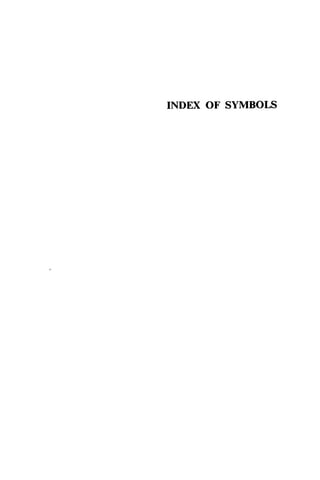

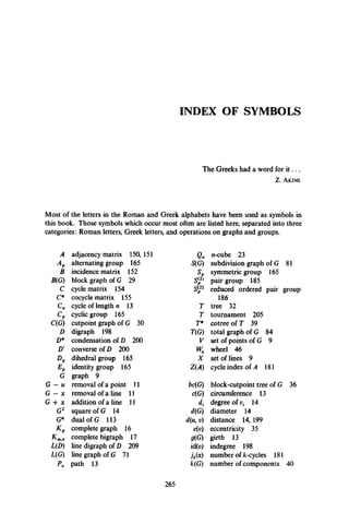
![266 INDEX OF SYMBOLS
m(G) cycle rank 39 <s> induced subgraph 11
m*(G) cocycle rank 39 Gi u G2 union of graphs 21
od(i;) outdegree 198 Gi + G2 join of graphs 21
P number of points 9 A + B sum of groups 163
(a q) p points, q lines 9 Gi x G2 product of graphs 21
q number of lines 9 A x B product of groups 163
fiG) radius 35 Gl[G2] composition of graphs 22
U , l W points 9 A[B composition of groups 164
x, y, z lines 9 Gj a G2 conjunction of graphs 25
BA power group 164
point covering number 94 G1° G2 corona of graphs 167
a! line covering number 94
/?0 point independence number
95
/?! line independence number
95
y genus 117
T(G) group of G 161
T^G) line group of G 161
S minimum degree 14
A maximum degree 14
0 thickness 120
k connectivity 43
k ( u , v) local connectivity 49
2 line-connectivity 43
v crossing number 122
coarseness 121
n(G) partition of a graph 57
Y(G) arboricity 90
X chromatic number 127
X' line-chromatic number 133
ij/ achromatic number 144
a> intersection number 19
Q(F) intersection graph 19](https://image.slidesharecdn.com/graphtheory-181103155731/85/Graph-theory-277-320.jpg)
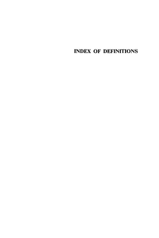

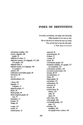
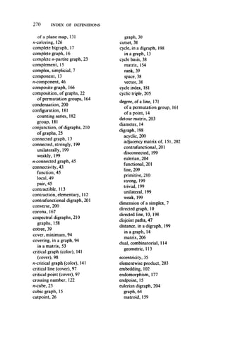
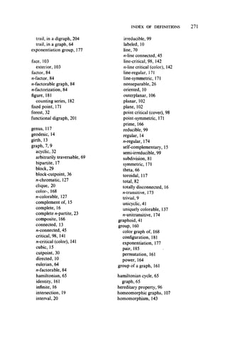
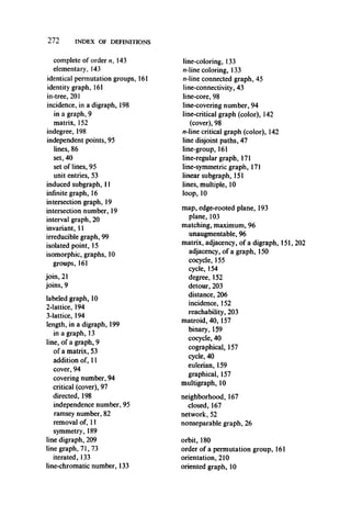

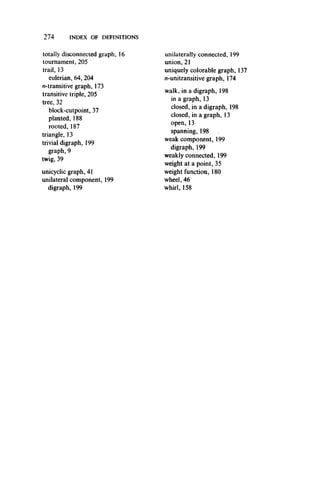

This document provides a brief history of the discovery of graph theory. It begins with Euler solving the Konigsberg bridge problem in 1736, replacing the land areas and bridges with a graph. This is considered the first recorded use of graphs. Later, Kirchhoff developed concepts of trees in graphs to solve electric networks. Cayley also considered trees arising from chemical isomers. The Four Color Conjecture then came to prominence. Graph theory has since been rediscovered many times with applications in diverse fields.