A perfect matching in a bipartite graph is a matching that matches all vertices. The document discusses algorithms for finding a perfect matching in regular bipartite graphs. The currently most efficient algorithm takes time O(m), where m is the number of edges and n is the number of vertices. The document improves this to O(min{m, n2.5ln n/d}) by proving a uniform sampling theorem: sampling each edge independently with probability O(n ln n/d2) results in a graph that has a perfect matching with high probability.

1. GRAPH<br />Definitions: <br />In mathematics, a Graph is an abstract representation of a set of objects where some pairs of the objects are connected by links. The interconnected objects are represented by mathematical abstractions called vertices, and the links that connect some pairs of vertices are called edges. Typically, a graph is depicted in diagrammatic form as a set of dots for the vertices, joined by lines or curves for the edges. Graphs are one of the objects of study in discrete mathematics. <br />74295066040 <br />The edges may be directed (asymmetric) or undirected (symmetric). For example, if the vertices represent people at a party, and there is an edge between two people if they shake hands, then this is an undirected graph, because if person A shook hands with person B, then person B also shook hands with person A. On the other hand, if the vertices represent people at a party, and there is an edge from person A to person B when person A knows of person B, then this graph is directed, because knowing of someone is not necessarily a symmetric relation (that is, one person knowing of another person does not necessarily imply the reverse; for example, many fans may know of a celebrity, but the celebrity is unlikely to know of all their fans). This latter type of graph is called a directed graph and the edges are called directed edges or arcs; in contrast, a graph where the edges are not directed is called undirected.<br />Vertices are also called nodes or points, and edges are also called lines. Graphs are the basic subject studied by graph theory. A graph consists of a set of nodes represented by small circles, and a set of arcs represented by lines. If a path can be found that connects all the nodes, then a graph is said to be a connected graph. If no pair of nodes is connected by more than one arc then the graph is said to be a simple graph. A graph in which each arc has an associated direction is a digraph<br />GRAPH THEORY <br />Explanations: <br />The word quot;
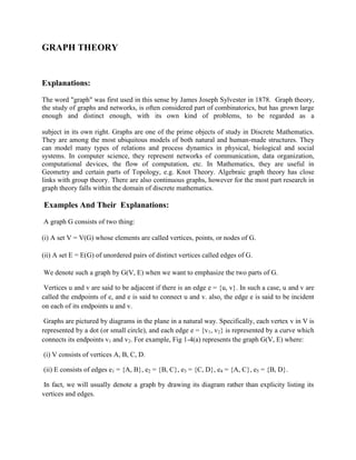
graphquot;
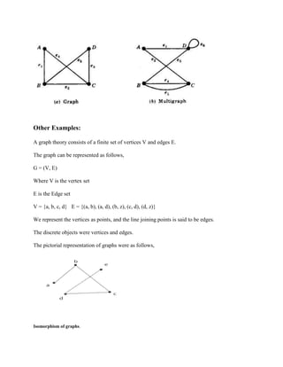
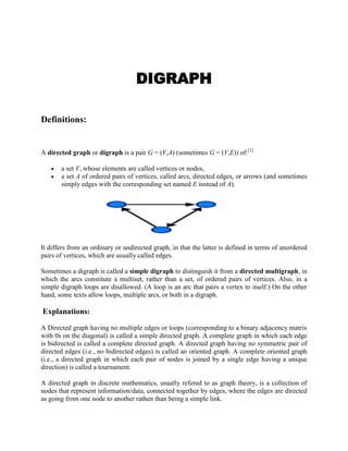
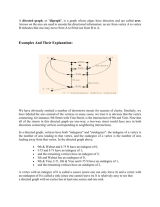
was first used in this sense by James Joseph Sylvester in 1878. Graph theory, the study of graphs and networks, is often considered part of combinatorics, but has grown large enough and distinct enough, with its own kind of problems, to be regarded as a<br />subject in its own right. Graphs are one of the prime objects of study in Discrete Mathematics. They are among the most ubiquitous models of both natural and human-made structures. They can model many types of relations and process dynamics in physical, biological and social systems. In computer science, they represent networks of communication, data organization, computational devices, the flow of computation, etc. In Mathematics, they are useful in Geometry and certain parts of Topology, e.g. Knot Theory. Algebraic graph theory has close links with group theory. There are also continuous graphs, however for the most part research in graph theory falls within the domain of discrete mathematics. <br /> Examples And Their Explanations: <br /> A graph G consists of two thing:<br />(i) A set V = V(G) whose elements are called vertices, points, or nodes of G.<br />(ii) A set E = E(G) of unordered pairs of distinct vertices called edges of G.<br /> We denote such a graph by G(V, E) when we want to emphasize the two parts of G.<br /> Vertices u and v are said to be adjacent if there is an edge e = {u, v}. In such a case, u and v are called the endpoints of e, and e is said to connect u and v. also, the edge e is said to be incident on each of its endpoints u and v.<br /> Graphs are pictured by diagrams in the plane in a natural way. Specifically, each vertex v in V is represented by a dot (or small circle), and each edge e = {v1, v2} is represented by a curve which connects its endpoints v1 and v2. For example, Fig 1-4(a) represents the graph G(V, E) where: <br /> (i) V consists of vertices A, B, C, D.<br /> (ii) E consists of edges e1 = {A, B}, e2 = {B, C}, e3 = {C, D}, e4 = {A, C}, e5 = {B, D}.<br /> In fact, we will usually denote a graph by drawing its diagram rather than explicity listing its vertices and edges. <br /> <br />Other Examples:<br />A graph theory consists of a finite set of vertices V and edges E.<br />The graph can be represented as follows,<br />G = (V, E)<br />Where V is the vertex set<br />E is the Edge set<br />V = {a, b, c, d} E = {(a, b), (a, d), (b, z), (c, d), (d, z)}<br />We represent the vertices as points, and the line joining points is said to be edges.<br />The discrete objects were vertices and edges.<br />The pictorial representation of graphs were as follows,<br />Isomorphism of graphs.<br />DIGRAPH<br />Definitions: <br />A directed graph or digraph is a pair G = (V,A) (sometimes G = (V,E)) of:[1]<br />a set V, whose elements are called vertices or nodes,<br />a set A of ordered pairs of vertices, called arcs, directed edges, or arrows (and sometimes simply edges with the corresponding set named E instead of A).<br />135255077470 <br /> <br />It differs from an ordinary or undirected graph, in that the latter is defined in terms of unordered pairs of vertices, which are usually called edges.<br />Sometimes a digraph is called a simple digraph to distinguish it from a directed multigraph, in which the arcs constitute a multiset, rather than a set, of ordered pairs of vertices. Also, in a simple digraph loops are disallowed. (A loop is an arc that pairs a vertex to itself.) On the other hand, some texts allow loops, multiple arcs, or both in a digraph.<br /> Explanations: <br />A Directed graph having no multiple edges or loops (corresponding to a binary adjacency matrix with 0s on the diagonal) is called a simple directed graph. A complete graph in which each edge is bidirected is called a complete directed graph. A directed graph having no symmetric pair of directed edges (i.e., no bidirected edges) is called an oriented graph. A complete oriented graph (i.e., a directed graph in which each pair of nodes is joined by a single edge having a unique direction) is called a tournament. <br />A directed graph in discrete mathematics, usually refered to as graph theory, is a collection of nodes that represent information/data, connected together by edges, where the edges are directed as going from one node to another rathen than being a simple link. <br />A directed graph, or quot;
digraphquot;
, is a HYPERLINK quot;
http://www.rwc.uc.edu/koehler/comath/31.htmlquot;
graph whose edges have direction and are called arcs. Arrows on the arcs are used to encode the directional information: an arc from vertex A to vertex B indicates that one may move from A to B but not from B to A. <br />Examples And Their Explanation: <br />971550304166<br /> <br /> <br /> <br />We have obviously omitted a number of downtown streets for reasons of clarity. Similarly, we have labeled the arcs instead of the vertices in many cases; we trust it is obvious that the vertex connecting, for instance, 9th Street with Vine Street, is the intersection of 9th and Vine. Note that all of the streets in this directed graph are one-way; a two-way street would have arcs in both directions connecting vertices corresponding to neighboring intersections. <br />In a directed graph, vertices have both quot;
indegreesquot;
and quot;
outdegreesquot;
: the indegree of a vertex is the number of arcs leading to that vertex, and the outdegree of a vertex is the number of arcs leading away from that vertex. In the directed graph above, <br />9th & Walnut and I-75 N have an indegree of 0,<br />I-75 and I-71 have an indegree of 1,<br />and the remaining vertices have an indegree of 2;<br />5th and Walnut has an outdegree of 0,<br />9th & Vine, I-71, 8th & Vine and I-75 N have an outdegree of 1,<br />and the remaining vertices have an outdegree of 2. <br />A vertex with an indegree of 0 is called a source (since one can only leave it) and a vertex with an outdegree of 0 is called a sink (since one cannot leave it). It is relatively easy to see that <br />a directed graph with no cycles has at least one source and one sink. <br /> <br />BIPARTITE GRAPH And PERFECT MATCHING<br />Definitions: <br />The bipartite graphs is the topic coming under graph theory.We will study bipartite graphs online here.The bipartite graphs are the sub category of k-partite graph.<br />First,we will define the word bipartite,the bipartite graph is a graph ,of which the vertices can be divided in to two disjoint sets.<br />In a bipartite graph we can divide the vertex sets to 2 sets u and v which are disjoint , and independent sets.<br />And a bipartite graph wont contain any odd cycles.<br />If we go in to graph coloring each of the sets of disjoint setrs will be in one color,which is not possible in non bipartite graph.<br />Some bipartite graphs:<br />1.all trees are bipartite<br />2.The cyclic graphs with even number of vertices are bipartite.<br /> Explanations: <br />Bipartite graphs also known as the bigraphs are the type of graphs having the collection of vertices in the form of two disjoint sets , such that the vertices within the same set will never be adjacent. <br />These are classified into two ways :<br />Simple Bipartite graph : in which all vertices of first set need not to be connected to vertices of second set.<br />Complete Bipartite graph : in which every vertex of the first set must be connected to every vertex of second set.<br /> <br />Examples of Bipartite Graphs: <br />Example 1:<br />Solve the vertices and the edges of the bipartite graph.<br />Solution:<br /> In this graph, the value of m = 5 and the n = 3.<br />Vertices = n + m.<br /> = 5 +3.<br /> = 8.<br /> Edges = m * n.<br /> = 5 * 3.<br /> = 15.<br />This is the solution of bipartite graph.<br />Example 2:<br />Find the vertices and the edges of the following graph.<br />Solution:<br /> In this graph, m= 3 and n=3.<br />Vertices = m + n.<br /> = 3 + 3.<br /> = 6.<br /> Edges = n * m.<br /> = 3 * 3<br /> = 9.<br /> This is the solution of bipartite graph.<br />Other Examples And Their Explanations: <br /> <br /> Example 1: Determine the number of vertices in the bipartite graph given.<br />Solution : As it is seen that the first set has 4 vertices and the second has 5 vertices , so<br />Total vertices = 4 + 5 = 9 vertices.<br />Example 2 : Determine the number of edges as well as vertices in the bipartite graph given.<br />Solution : As it is seen that the first set m has 3 vertices and the second n has 3 vertices , so<br />Total vertices = m + n =3 + 3 = 6 vertices.<br />As given graph is a complete bipartite graph , so number of edges<br />Total edges = m * n = 3 * 3 = 9 edges<br />Example 3 : Determine the number of vertices in the bipartite graph given.<br />Solution : As it is seen that the first set has 4 vertices and the second has 4 vertices , so<br />Total vertices = 4 + 4 = 8 vertices.<br />Example 4 : Determine the number of edges as well as vertices in the bipartite graph given. <br />Solution : As it is seen that the first set m has 5 vertices and the second n has 4 vertices , so<br />Total vertices = m + n =5+4 = 9 vertices.<br />As given graph is a complete bipartite graph , so number of edges<br />Total edges = m * n = 5 * 4 = 20 edges<br />Perfect matching<br />Explanations: <br />We give lower and upper bounds for the number of reducible ears as well as upper bounds for the number of perfect matchings in an elementary bipartite graph. An application to chemical graphs is also discussed. In addition, a method to construct all minimal elementary bipartite graphs is described.<br />we further investigate the well-studied problem of finding a perfect matching in a regular bipartite graph. The first nontrivial algorithm, with running time O(mn), dates back to König's work in 1916 (here m&equals;nd is the number of edges in the graph, 2n is the number of vertices, and d is the degree of each node). The currently most efficient algorithm takes time O(m), and is due to Cole et al. &lsqb;2001&rsqb;. We improve this running time to O(min{m, n2.5ln n/d}); this minimum can never be larger than O(n1.75&sqrt;ln n). We obtain this improvement by proving a uniform sampling theorem: if we sample each edge in a d-regular bipartite graph independently with a probability p &equals; O(n ln n/d2) then the resulting graph has a perfect matching with high probability. The proof involves a decomposition of the graph into pieces which are guaranteed to have many perfect matchings but do not have any small cuts. We then establish a correspondence between potential witnesses to nonexistence of a matching (after sampling) in any piece and cuts of comparable size in that same piece. Karger's sampling theorem &lsqb;1994a, 1994b&rsqb; for preserving cuts in a graph can now be adapted to prove our uniform sampling theorem for preserving perfect matchings. Using the O(m&sqrt;n) algorithm (due to Hopcroft and Karp &lsqb;1973&rsqb;) for finding maximum matchings in bipartite graphs on the sampled graph then yields the stated running time. We also provide an infinite family of instances to show that our uniform sampling result is tight up to polylogarithmic factors (in fact, up to ln2 n). <br /> <br />