Chapter 11

CHAPTER 11
LATERAL EARTH PRESSURE
11.1 INTRODUCTION
Structures that are built to retain vertical or nearly vertical earth banks or any other material are
called retaining walls. Retaining walls may be constructed of masonry or sheet piles. Some of the
purposes for which retaining walls are used are shown in Fig. 11.1.
Retaining walls may retain water also. The earth retained may be natural soil or fill. The
principal types of retaining walls are given in Figs. 11.1 and 11.2.
Whatever may be the type of wall, all the walls listed above have to withstand lateral
pressures either from earth or any other material on their faces. The pressures acting on the walls try
to move the walls from their position. The walls should be so designed as to keep them stable in
their position. Gravity walls resist movement because of their heavy sections. They are built of
mass concrete or stone or brick masonry. No reinforcement is required in these walls. Semi-gravity
walls are not as heavy as gravity walls. A small amount of reinforcement is used for reducing the
mass of concrete. The stems of cantilever walls are thinner in section. The base slab is the cantilever
portion. These walls are made of reinforced concrete. Counterfort walls are similar to cantilever
walls except that the stem of the walls span horizontally between vertical brackets known as
counterforts. The counterforts are provided on the backfill side. Buttressed walls are similar to
counterfort walls except the brackets or buttress walls are provided on the opposite side of the
backfill.
In all these cases, the backfill tries to move the wall from its position. The movement of the
wall is partly resisted by the wall itself and partly by soil in front of the wall.
Sheet pile walls are more flexible than the other types. The earth pressure on these walls is
dealt with in Chapter 20. There is another type of wall that is gaining popularity. This is
mechanically stabilized reinforced earth retaining walls (MSE) which will be dealt with later on.
This chapter deals with lateral earth pressures only.
419

420 Chapter 11
(c) A bridge abutment (d) Water storage
.VI
(e) Flood walls (f) Sheetpile wall
Figure 11.1 Use of retaining walls
11.2 LATERAL EARTH PRESSURE THEORY
There are two classical earth pressure theories. They are
1. Coulomb's earth pressure theory.
2. Rankine's earth pressure theory.
The first rigorous analysis of the problem of lateral earth pressure was published
by Coulomb in (1776). Rankine (1857) proposed a different approach to the problem.
These theories propose to estimate the magnitudes of two pressures called active earth pressure
and passive earth pressure as explained below.
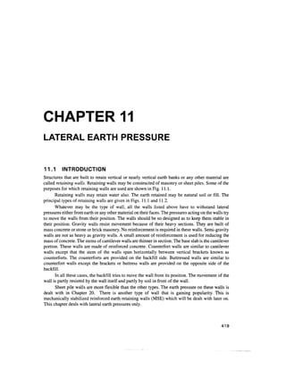
Consider a rigid retaining wall with a plane vertical face, as shown in Fig. 11.3(a), is
backfilled with cohesionless soil. If the wall does not move even after back filling, the pressure
exerted on the wall is termed as pressure for the at rest condition of the wall. If suppose the wall
gradually rotates about point A and moves away from the backfill, the unit pressure on the wall is
gradually reduced and after a particulardisplacement of the wall at the top,the pressure reaches a
constant value. The pressure is the minimumpossible. This pressure is termed the active pressure
since the weight of the backfill is responsible for the movement of the wall. If the wall is smooth,

Lateral Earth Pressure 421
Base slab
Heel
(a) Gravity walls (b) Semi-gravity walls (c) Cantilever walls
Backfill Counterfort Face of wall —i
— Buttress
Face
of wall
(d) Counterfort walls (e) Buttressed walls
Figure 11.2 Principal types of rigid retaining walls
the resultant pressure acts normal to the face of the wall. If the wall is rough, it makes an angle <5
with the normal on the wall. The angle 8 is called the angle of wallfriction. As the wall moves away
from the backfill, the soil tends to move forward.When the wall movement is sufficient, a soil mass
of weight W ruptures along surface ADC shown in Fig. 11.3(a). This surface is slightly curved. If
the surface is assumed to be a plane surface AC, analysis would indicate that this surface would
make an angle of 45° + 0/2 with the horizontal.
If the wall is now rotated about A towards the backfill, the actual failure plane ADC is also a
curved surface [Fig. 11.3(b)]. However, if the failure surface is approximated as a plane AC, this
makes an angle 45° - 0/2 with the horizontal and the pressure on the wall increases from the value
of the at rest condition to the maximumvalue possible. The maximum pressure P that is developed
is termed the passive earth pressure. The pressure is called passive because the weight of the
backfill opposes the movement of the wall. It makes an angle 8 with the normal if the wall is rough.
The gradual decrease or increase of pressure on the wall with the movement of the wall from
the at rest condition may be depicted as shown in Fig. 11.4.
The movement A required to develop the passive state is considerably larger than AQ required
for the active state.
11.3 LATERAL EARTH PRESSURE FOR AT REST CONDITION
If the wall is rigid and does not move with the pressure exerted on the wall, the soil behind the wall
will be in a state of elastic equilibrium. Consider a prismatic element E in the backfill at depth z
shown in Fig. 11.5.
Element E is subjected to the following pressures.
Vertical pressure = crv= yz; lateral pressure = <Jh

422 Chapter 11
(a) Active earth pressure
(b) Passive earth pressure
Figure 11.3 Wall movement for the development of active and passive earth
pressures
where yis the effective unit weight of the soil. If we consider the backfill is homogeneous then both
cry and oh increase linearly with depth z. In such a case, the ratio of ah to <JV remains constant with
respect to depth, that is
—- = —- = constant = AT,
cr yz (11-1)
where KQ is called the coefficient of earth pressurefor the at rest condition or at rest earth pressure
coefficient.
The lateral earth pressure oh acting on the wall at any depth z may be expressed as
cr, - (11.la)

Passive pressure
Away from backfill Into backfill
Figure 11.4 Development of active and passive earth pressures
H
z z
H/3
L
A
Ph = K
tiYZ
(a) (b)
Figure 11.5 Lateral earth pressure for at rest condition
The expression for oh at depth H, the height of the wall, is
The distribution of oh on the wall is given in Fig. 11.5(b).
The total pressure PQ for the soil for the at rest condition is
(11.Ib)
(11.lc)

424 Chapter 11
Table 11.1 Coefficients of earth pressure for at rest condition
Type of soil / KQ
Loose sand, saturated
Dense sand, saturated
Dense sand, dry (e =0.6) -
Loose sand, dry (e =0.8) -
Compacted clay 9
Compacted clay 31
Organic silty clay, undisturbed (w{ = 74%) 45
0.46
0.36
0.49
0.64
0.42
0.60
0.57
The value of KQ depends upon the relative density of the sand and the process by which the
deposit was formed. If this process does not involve artificial tamping the value of KQ ranges from
about 0.40 for loose sand to 0.6 for dense sand. Tamping the layers may increase it to 0.8.
The value of KQ may also be obtained on the basis of elastic theory. If a cylindrical sample of soil
is acted upon by vertical stressCT,and horizontal stress ah, the lateral strain e{ may be expressed as
(11.2)
where E =Young's modulus, n =Poisson's ratio.
The lateral strain e{ = 0 when the earth is in the at rest condition. For this condition, we may
write
a
h V
or — =— (11.3)
where ~T^~ = KQ, crv=yz (11.4)
According to Jaky (1944), a good approximation for K0 is given by Eq. (11.5).
KQ=l-sin0 (11.5)
which fits most of the experimental data.
Numerical values of KQ for some soils are given in Table 11.1.
Example 11.1
If a retaining wall 5 m high is restrained from yielding, what will be the at-rest earth pressure per
meter length of the wall? Given: the backfill is cohesionless soil having 0 = 30° and y= 18 kN/m3
.
Also determine the resultant force for the at-rest condition.
Solution
From Eq. (11.5)
KQ = l-sin^= l-sin30° =0.5
From Eq. (1Lib), ah =KjH - 0.5 x 18x 5 = 45 kN/m2

From Eq. (ll.lc)
PQ = - KQy H2
=~ x 0.5x 18x 52
= 112.5 kN/m length of wall
11.4 RANKINE'S STATES OF PLASTIC EQUILIBRIUM FOR
COHESIONLESS SOILS
Let ATin Fig. 11.6(a) represent the horizontal surface of a semi-infinite mass of cohesionless soil
with a unit weight y. The soil is in an initial state of elastic equilibrium. Consider a prismatic block
ABCD. The depth of the block is z and the cross-sectional area of the block is unity. Since the
element is symmetrical with respect to a vertical plane, the normal stress on the base AD is
°V=YZ (11.6)
o~v is a principal stress. The normal stress oh on the vertical planes AB or DC at depth z may be
expressed as a function of vertical stress.
<rh
=
f(°v) =K
orz (H.7)
where KQ is the coefficient of earth pressure for the at rest condition which is assumed as a constant
for a particular soil. The horizontal stress oh varies from zero at the ground surface to KQyz at
depth z.
Expansion 45° +
D A
T TTTT
Direction of
major principal
stress Stress lines
(a) Active state
Compression
X
K0yz
— Kpyz
Direction of
minor principal
stress
(b) Passive state
Direction of
minor principal
stress
Direction of
major principal
stress
Figure 11.6(a, b) Rankine's condition for active and passive failures in a semi-
infinite mass of cohesionless soil

426 Chapter 11
B' B C B B' C
Failure
plane
H
45° + 0/2
Failure
plane
45°-0/2
(c) Local active failure (d) Local passive failure
A45°+0/2
Cn
(e) Mohr stress diagram
Figure 11.6(c, d, e) Rankine's condition for active and passive failures in a semi-
infinite mass of cohesionless soil
If we imagine that the entire mass is subjected to horizontal deformation, such deformation is
a plane deformation. Every vertical section through the mass represents a plane of symmetry for the
entire mass. Therefore, the shear stresses on vertical and horizontal sides of the prism are equal to
zero.
Due to the stretching, the pressure on vertical sides AB and CD of the prism decreases until
the conditions of plastic equilibrium are satisfied, while the pressure on the base AD remains
unchanged. Any further stretching merely causes a plastic flow without changing the state of stress.
The transition from the state of plastic equilibrium to the state of plastic flow represents the failure
of the mass. Since the weight of the mass assists in producing an expansion in a horizontal
direction, the subsequent failure is called active failure.
If, on the other hand, the mass of soil is compressed, as shown in Fig. 11.6(b), in a horizontal
direction, the pressure on vertical sides AB and CD of the prism increases while the pressure on its
base remains unchanged at yz. Since the lateral compression of the soil is resisted by the weight of
the soil, the subsequent failure by plastic flow is called apassive failure.

The problem now consists of determining the stresses associated with the states of plastic
equilibrium in the semi-infinite mass and the orientation of the surface of sliding. The problem was
solved by Rankine (1857).
The plastic states which are produced by stretching or by compressing a semi-infinitemass of
soil parallel to its surface are called active and passive Rankine states respectively. The orientation
of the planes may be found by Mohr's diagram.
Horizontal stretching or compressing of a semi-infinite mass to develop a state of plastic
equilibrium is only a concept. However, local states of plastic equilibrium in a soil mass can be
created by rotating a retaining wall about its base either away from the backfill for an active state or
into the backfill for a passive state in the way shown in Figs. 1 1.3(c) and (d) respectively. In both
cases, the soil within wedge ABC will be in a state of plastic equilibrium and lineAC represents the
rupture plane.
Mohr Circle for Active and Passive States of Equilibrium in Granular Soils
Point P{ on the d-axis in Fig. 1 1.6(e) represents the state of stress on base AD of prismatic element
ABCD in Fig. 1 1.6(a). Since the shear stress on AD is zero, the vertical stress on the base
is a principal stress. OA and OB are the two Mohr envelopes which satisfy the Coulomb equation of
shear strength
j = crtan^ (11.9)
Two circles Ca and C can be drawn passing through Pl and at the same time tangential to the Mohr
envelopes OA and OB. When the semi-infinite mass is stretched horizontally, the horizontal stress
on vertical faces AB and CD (Fig. 1 1.6 a) at depth z is reduced to the minimum possible and this
stress is less than vertical stress ov.Mohr circle Ca gives the state of stress on the prismatic element
at depth z when the mass is in active failure. The intercepts OPl and OP2 are the major and minor
principal stresses respectively.
When the semi-infinite mass is compressed (Fig. 1 1.6 b), the horizontal stress on the vertical
face of the prismatic element reaches the maximum value OP3 and circle C is the Mohr circle
which gives that state of stress.
Active State of Stress
From Mohr circle Ca
Major principal stress = OP{ = crl = yz
Minor principal stress = OP2 = <73
(7, + <J~, <J, — (To
nn —
JJ, —
1
2
cr. —<TT <j, + CT-,
From triangle 00,C,, — = — sin i
1 J
2 2
( 1 + sin 0|
"

Therefore, pa =cr3 =—-= yzKA (U.ll)
'V
where a, = yz, KA =coefficient of earth pressure for the active state =tan2
(45° - 0/2).

428 Chapter 11
From point Pr draw a line parallel to the base AD on which (7{ acts. Since this line coincides
with the cr-axis, point P9 is the origin of planes. Lines P2C{ and P^C giye tne
orientations of the
failure planes. They make an angle of 45° + 0/2 with the cr-axis.The lines drawn parallel to the lines
P2Cj and P2C'{ in Fig. 11.6(a) give the shear lines along which the soil slips in the plastic state. The
angle between a pair of conjugate shear lines is (90° - 0).
Passive State of Stress
C is the Mohr circle in Fig. (11.6e) for the passive state and P3 is the origin of planes.
Major principal stress = (j} =p = OP^
Minor principal stress = (73 = OPl = yz.
From triangle OO^C2, o{ = yzN^
Since <Jl - p and <J3 = yz, we have
n -yzN:-r7K (]] ]?}
i n * Q) i ft L L * . £ j
where K = coefficient of earth pressure for the passive state = tan2
(45° + 0/2).
The shear failure lines are P3C2 and P3C^ and they make an angle of 45° - 0/2 with the
horizontal. The shear failure lines are drawn parallel to P3C2 and P3C'2 in Fig. 11.6(b). The angle
between any pair of conjugate shear lines is (90° + 0).
11.5 RANKINE'S EARTH PRESSURE AGAINST SMOOTH
VERTICAL WALL WITH COHESIONLESS BACKFILL
Backfill Horizontal-Active Earth Pressure
Section AB in Fig. 11.6(a) in a semi-infinitemass is replaced by a smooth wall AB in Fig. 11.7(a).
The lateral pressure acting against smooth wall AB is due to the mass of soil ABC above
failure line AC which makes an angle of 45° + 0/2 with the horizontal. The lateral pressure
distribution on wall AB of height H increases in simple proportion to depth. The pressure acts
normal to the wall AB [Fig. 11.7(b)].
The lateral active pressure at A is
(11.13)
B' B
W
45° +
(a) (b)
Figure 11.7 Rankine's active earth pressure in cohesionless soil

The total pressure on AB is therefore
H H
z d Z = K
(11.14)
o o
where, KA =tan2
(45° -
1+ sin^ Vi
Pa acts at a height H/3 above the base of the wall.
Backfill Horizontal-Passive Earth Pressure
If wall AB is pushed into the mass to such an extent as to impart uniform compression throughout
the mass, soil wedge ABC in Fig. 11.8(a) will be in Rankine's passive state of plastic equilibrium.
The inner ruptureplane ACmakes an angle 45° + 0/2 with the vertical AB. The pressure distribution
on wall AB is linear as shown in Fig. 11.8(b).
The passive pressure p at A is
PP=YHKp
the total pressure against the wall is
P
P = (11.15)
where, Kp = tan2
(45° +
1+ sin^
1- sin 6
Relationship between Kp and KA
The ratio of Kp and KA may be written as
Kp tan2
(45c
KA tan2
(45c (11.16)
B B'
Inner rupture plane
' W
(a) (b)
Figure 11.8 Rankine's passive earth pressure in cohesionless soil

430 Chapter 11
H
P + P
1
aTr
w
45° + 0/2
(a) Retaining wall
'-*
H- vbnKA
(b) Pressure distribution
H
Figure 11.9 Rankine's active pressure under submerged condition in cohesionless
soil
For example, if 0 = 30°, we have,
K
P
-7T1
= tan4
600
=9, or Kp=9KA
KA
This simple demonstration indicates that the value of Kp is quite large compared to KA.
Active Earth Pressure-Backfill Soil Submerged with the Surface Horizontal
When the backfill is fully submerged, two types of pressures act on wall AB. (Fig. 1 1.9) They are
1. The active earth pressure due to the submerged weight of soil
2. The lateral pressure due to water
At any depth z the total unit pressure on the wall is
At depth z = H, we have
~p~ = y,HK. + y H
r a ID A ' w
where yb is the submerged unit weight of soil and yw the unit weight of water. The total pressure
acting on the wall at a height H/3 above the base is
(11.17)
Active Earth Pressure-Backfill Partly Submerged with a Uniform Surcharge Load
The ground water table is at a depth of Hl below the surface and the soil above this level has an
effective moist unit weight of y.The soil below the water table is submerged with a submerged unit
weight yb. In this case, the total unit pressure may be expressed as given below.
At depth Hl at the level of the water table

At depth H we have
or (11.18)
The pressure distribution is given in Fig. 1 1.10(b). It is assumed that the value of 0 remains
the same throughout the depth H.
From Fig. 1 1.10(b), we may say that the total pressure Pa acting per unit length of the wall
may be written as equal to
(11.19)
The point of application of Pa above the base of the wall can be found by taking moments of
all the forces acting on the wall about A.
Sloping Surface-Active Earth Pressure
Figure 1 1.11 (a) shows a smooth vertical wall with a sloping backfill of cohesionless soil. As in the
case of a horizontal backfill, the active state of plastic equilibrium can be developed in the backfill
by rotating the wall about A away from the backfill. Let AC be the rupture line and the soil within
the wedge ABC be in an active state of plastic equilibrium.
Consider a rhombic element E within the plastic zone ABC which is shown to a larger scale
outside. The base of the element is parallel to the backfill surface which is inclined at an angle /3to
the horizontal. The horizontal width of the element is taken as unity.
Let o~v = the vertical stress acting on an elemental length ab =
(7l = the lateral pressure acting on vertical surface be of the element
The vertical stress o~v can be resolved into components <3n the normal stress and t the shear
stress on surface ab of element E. We may now write
H
g/unit area
I I I 1 I I
I
Pa (total) =
(a) Retaining wall (b) Pressure distribution
Figure 11.10 Rankine's active pressure in cohesionless backfill under partly
submerged condition with surcharge load

432 Chapter 11
H
O CT3 0, On O]
(c) Mohr diagram
Figure 11.11 Rankine's active pressure for a sloping cohesionless backfill
n - <Jv cos fi = yz cos /?cos fl=yz cos2
j3
T = a sin/? =
(11.20)
(11.21)
A Mohr diagram can be drawn as shown in Fig. 11.1l(c). Here, length OA = yzcos/3 makes
an angle (3 with the (T-axis. OD =on - yzcos2
/3 and AD =T= yzcosf} sin/3. OM is the Mohr envelope
making an angle 0 with the <7-axis. Now Mohr circle C} can be drawn passing through point A and
at the same time tangential to envelope OM. This circle cuts line OA at point B and theCT-axisat E
andF.
Now OB = the lateral pressure ol =pa in the active state.
The principal stresses are
OF = CTj and OE = a3
The following relationships can be expressed with reference to the Mohr diagram.
BC = CA= —-l -sm2
j3

= OC-BC =
2
cr, +CT, cr, + cr,
i
2 2
Now we have (after simplification)
cos 0-T] cos2
ft -cos
crv yzcosfi cos 0+ J cos2
fi - cos2
0
or
cos B- A/cos2
/?- cos2
(b
- v
cos/?+cos2
/?-cos
where, K. = cos fix
(11.22)
(11.23)
(11.24)
is called as the coefficient of earth pressure for the active state or the active earth pressure
coefficient.
The pressure distribution on the wall is shown in Fig. 1 1 .1 l(b). The active pressure at depthH
is
which acts parallel to the surface. The total pressure PQ per unit length of the wall is
(11.25)
which acts at a height H/3 from the base of the wall and parallel to the sloping surface of the
backfill.
Figure 11.12 Rankine's passive pressure in sloping cohesionless backfill

434 Chapter 11
Sloping Surface-Passive Earth Pressure (Fig. 11.12)
An equation for P for a sloping backfill surface can be developed in the same way as for an active
case. The equation for P may be expressed as
(11.26)
n cosfi+ Jcos2
fl- cos2
0
where, Kp=cos]3x /
cos/3 - ^cos2
j3- cos2
0
P acts at a height H/3 above point A and parallel to the sloping surface.
(11.27)
Example 11.2
A cantilever retaining wall of 7 meter height (Fig. Ex. 11.2) retains sand. The properties of the sand
are: e - 0.5, 0 = 30° and G^ =2.7. Using Rankine's theory determine the active earth pressure at the
base when the backfill is (i) dry, (ii)saturated and (iii)submerged, and also the resultant active force
in each case. In addition determine the total water pressure under the submerged condition.
Solution
e =0.5andG = 2.7, y, = -^ = —— x9.81 = 17.66 kN/m3
d
l +e 1 +0.5
Saturated unit weight
Backfill submerged
Backfill saturated
Water pressure
pa =48.81 kN/m"
= 68.67 kN/m2
=Pw
Figure Ex. 11.2

=
sat
l +e 1 +0.5
Submerged unit weight
rb =rsal -rw=20.92-9.81 =11.1 kN/m3
l-sin^ 1- sin 30° 1
For* =30, *A
Active earth pressure at the base is
(i) for dry backfill
Pa =
P =-KA r,H2
=-x 41.2x7 = 144.2 kN/mofwall
a r A ' a rj
(ii) for saturated backfill
Pa =K
A Ysat H =-x 20.92 x 7 = 48.81kN/m2
p = -x 48.81x7 = 170.85 kN/m ofwall
a
2
(in) for submerged backfill
Submerged soil pressure
Pa
=K
/JbH
=- x 1 1.1x7 = 25.9kN/m2
P = - x 25.9 x7= 90.65 kN/ m ofwall
a
2
Water pressure
pw =ywH =9.81 x7 = 68.67 kN/m2
Pw=-YwH2
= -x 9.81x72
=240.35 kN/mofwall
Example 11.3
For the earth retaining structure shownin Fig.Ex. 11.3, construct the earth pressure diagram for the
active state and determine the total thrust per unit length of the wall.
Solution
1-sin 30° 1
For<z)=30°, KA : - = -
G Y 265 i
Dry unit weight YH =—^^ = —: x
62.4= 100.22 lb/ fr
y d
l +e 1 +0.65

436 Chapter 11
q = 292 lb/ft2
J I U J J H J
E--
//A
|
= i
32.8ft >>
1
1
J
1
9.8ft
Sand Gs =2.65
e =0.65
0 =30°
(a) Given system
Pl Pi P3
(b) Pressure diagram
Figure Ex. 11.3
(Gs-l)yw 2.65-1
7b =-^—-=T-^X 62.4= 62.4 ,b/f,3
Assuming the soil above the water table is dry,[Refer to Fig.Ex. 11.3(b)].
P! = KAydHl =-x 100.22x9.8 = 327.39 lb/ft2
p2 = KAybH2 =- x 62.4 x 23 = 478.4 lb/ft2
p3 = KAxq =-x292 =97.33 lb/ft2
P4 = (K
A^wrw
H
2 = 1x62.4x23 = 1435.2 lb/ft2
Total thrust = summation of the areas of the different parts of the pressure diagram
1 1 1
= ^PiHl+plH2+-p2H2+p3(Hl+H2) + -p4H2
= -x 327.39 x 9.8 + 327.39 x 23+-x 478.4 x 23 + 97.33(32.8) +-x 1435.2x23
2 2 2
= 34,333 lb/ft = 34.3kips/ft of wall
Example 11.4
A retaining wall with a vertical back of height 7.32m supports a cohesionless soil of unit weight
17.3 kN/m3
and an angle of shearing resistance 0 = 30°. The surface of the soil is horizontal.
Determine the magnitude and direction of the active thrust per meter of wall using Rankine
theory.

Solution
For the condition given here, Rankine's theory disregards the friction between the soil and the back
of the wall.
The coefficient of active earth pressure KA is
1-sind l-sin30° 1
Tf T_
A
1 + sin^ 1 +sin 30° 3
The lateral active thrust Pa is
Pa =-KAyH2
=-x-x 17.3(7.32)2
= 154.5 kN/m
Example 11.5
A rigid retaining wall 5 m high supports a backfill of cohesionless soil with 0= 30°. The water table
is below the base of the wall. The backfill is dry and has a unit weight of 18 kN/m3
. Determine
Rankine's passive earth pressure per meter length of the wall (Fig.Ex. 11.5).
Solution
FromEq. (11.15a)
Kp =
1+ sin^ 1 + sin 30° 1 +0.5
in^ l-sin30° 1-0.5
At the base level, the passive earth pressure is
pp =KpyH =3x18x5 = 270 kN/m2
FromEq. (11.15)
Pp=- KPy H =- x 3x 1 8x 5 = 675kN/m length ofwall
The pressure distribution is given in Fig.Ex. 1 1.5.
Pressure distribution
Figure Ex. 11.5

438 Chapter 11
Example 11.6
A counterfort wall of 10 m height retains a non-cohesive backfill. The void ratio and angle of
internal friction of the backfill respectively are 0.70and 30° in the loose state and they are 0.40and
40° in the dense state. Calculate and compare active and passive earth pressures for both the cases.
Take the specific gravity of solids as2.7.
Solution
(i) In the loose state, e - 0.70which gives
/""* - . r i—j
= _I^L = __ x 9 gj = 15 6 kN/m3
d
l +e 1 + 0.7
c j. ™° v l-sin0 1-sin 30° 1 1
For 0 = 3 0 , K, -= =— ,and^0 = =3
' A -i * ' 1 * O /" o O i TS
1 +sin 30 3 K,
Max. pa =KAydH = - x 15.6 x 10= 52 kN/m2
Max. p = KpydH = 3 x 15.6 x 10 = 468 kN/m2
(ii) In the dense state, e = 0.40, which gives,
Y =-22—x 9.81 = 18.92 kN/m3
d
1 + 0.4
1-sin 40° 1
For 0 = 40°, K=- —— = 0.217, Kp =-— =4.6
y A
1 +sin 40° p
K.
f
Max.pfl =KAydH =0.217x18.92x10 = 41.1 kN/m2
and Max. p = 4.6 x 18.92 x 10 = 870.3 kN/m2
Comment: The comparison of the results indicates that densification of soil decreases the
active earth pressure and increases the passive earth pressure. This is advantageous in the sense that
active earth pressure is a disturbing force and passive earth pressure is a resisting force.
Example 11.7
A wall of 8 m height retains sand having a density of 1.936Mg/m3
and an angle of internal friction
of 34°. If the surface of the backfill slopes upwards at 15° to the horizontal, find the active thrust per
unit length of the wall. Use Rankine's conditions.
Solution
There can be two solutions: analytical and graphical. The analytical solution can be obtained from
Eqs. (11.25) and (11.24) viz.,

Figure Ex. 11.7a
where K. = cos ft x
cos/?- ycos2
ft- cos2
COS/?+ yCOS2
ft- COS2
(f)
where ft = 15°, cos/? = 0.9659 and cos2
ft = 0.933
and ^ = 34° gives cos2
(/) = 0.688
0.966 -VO.933- 0.688
= 0.31 1
Hence KA = 0.966 x .
A
0.966 + VO.933-0.688
y = 1.936x9.81 = 19.0 kN/m3
Hence Pa = -x0.311x!9(8)2
= 189 kN/mwall
Graphical Solution
Vertical stress at a depth z = 8 m is
7/fcos/?=19x8xcosl5° = 147 kN/m2
Now draw the Mohr envelope at an angle of 34° and the ground line at an angle of 15° with
the horizontal axis as shown in Fig.Ex. 1 1.7b.
Using a suitable scale plot OPl = 147 kN/m2
.
(i) the center of circle C lies on the horizontal axis,
(ii) the circle passes through point Pr and
(iii) the circle is tangent to the Mohr envelope

440 Chapter 11
Ground line
16 18x 10
Pressure kN/m
Figure Ex. 11.7b
The point P2 at which the circle cuts the ground line represents the lateral earth pressure. The length
OP2 measures 47.5 kN/m2
.
Hence the active thrust per unit length, Pa =- x 47.5 x 8 = 190kN/m
1 1.6 RANKINE'S ACTIVE EARTH PRESSURE WITH COHESIVE
BACKFILL
In Fig. 11.13(a) is shown a prismatic element in a semi-infinite mass with a horizontal surface. The
vertical pressure on the base AD of the element at depth z is
The horizontal pressure on the element when the mass is in a state of plastic equilibriummay
be determined by making use of Mohr's stress diagram [Fig. 11.13(b)].
Mohr envelopes O'A and O'E for cohesive soils are expressed by Coulomb's equation
s - c+ tan 0 (11.28)
Point Pj on the cr-axis represents the state of stress on the base of the prismatic element.
When the mass is in the active state cr, is the major principal stress Cfj. The horizontal stress oh is the
minor principal stress <73. The Mohr circle of stress Ca passing through P{ and tangential to the
Mohr envelopes O'A and O'B represents the stress conditions in the active state. The relation
between the two principal stresses may be expressed by the expression
(11.29)
(11.30)
<7, = <7,A
1 J V v y
Substituting O", = 72, <73 =pa and transposing we have
rz 2c

45° + 0/2
Stretching
45° + 0/2
D B
C A
'" ,-; ,-" ,-" ,-•; t-
^A'-^ i"j Z:J A'
Tensile
zone
Failure shear lines
(a) Semi-infinite mass
Shear lines
(b) Mohr diagram
Figure 11.13 Active earth pressure of cohesive soil with horizontal backfill on a
vertical wall
The active pressure pa = 0 when
yz 2c rt
(11.31)
that is, pa is zero at depth z, such that
At depth z = 0, the pressure pa is
2c
Pa - JTf^
(11.32)
(11.33)

442 Chapter 1 1
Equations (11.32) and (11.33) indicate that the active pressure pa is tensile between depth 0
and ZQ. The Eqs. (11.32) and (11.33) can also be obtained from Mohr circles CQ and Ct respectively.
Shear Lines Pattern
The shear lines are shown in Fig. 1 1 .13(a). Up to depth ZQ they are shown dotted to indicate that this
zone is in tension.
Total Active Earth Pressure on a Vertical Section
If AB is the vertical section [1 1.14(a)], the active pressure distribution against this section of height
H is shown in Fig.11.14(b) as per Eq. (1 1.30). The total pressure against the section is
H H H
yz 2c
Pa = PZdz= ~dz- -r==dz
o 0 ' 0 V A
0
H
The shaded area in Fig. 11.14(b) gives the total pressure Pa. If the wall has a height
the total earth pressure is equal to zero. This indicates that a vertical bank of height smaller than H
can stand without lateral support. //, is called the critical depth. However, the pressure against the
wall increases from - 2c/JN^ at the top to + 2c/jN^ at depth //,, whereas on the vertical face of
an unsupported bank the normal stress is zero at every point. Because of this difference, the greatest
depth of which a cut can be excavated without lateral support for its vertical sides is slightly smaller
than Hc.
For soft clay, 0 = 0, and N^= 1
therefore, Pa=±yH2
-2cH (11.36)
4c
and HC=
~^ (1L37)
Soil does not resist any tension and as such it is quite unlikely that the soil would adhere to the
wall within the tension zone of depth z0 producing cracks in the soil. It is commonly assumed that
the active earth pressure is represented by the shaded area in Fig. 11.14(c).
The total pressure on wall AB is equal to the area of the triangle in Fig.11.14(c) which is
equal to
1 yH 2c
D 1 yH 2c „ 2c
or F =
" H
"

Surcharge load q/unit area
B l l C
2c
8
jH 2c
q
q

% v% N
*
(a) (b) (c) (d)
Figure 11.14 Active earth pressure on vertical sections in cohesive soils
Simplifying, we have
1 2c2
2 N
*
For soft clay, 0 = 0
Pa = -yHl
It may be noted that KA = IN^
(11.38c)
(11.39)
Effect of Surcharge and Water Table
Effect of Surcharge
When a surcharge load q per unit area acts on the surface, the lateral pressure on the wall due to
surcharge remains constant with depth as shown in Fig. 11.14(d) for the active condition. The
lateral pressure due to a surcharge under the active state may be written as
The total active pressure due to a surcharge load is,
n _&
(11.40)
Effect of Water Table
If the soil is partly submerged, the submerged unit weight below the water table will have to be
taken into account in both the active and passive states.

444 Chapter 11
Figure 11.15(a) shows the case of a wall in the active state with cohesive material as backfill.
The water table is at a depth of Hl below the top of the wall. The depth of water is //2.
The lateral pressure on the wall due to partial submergence is due to soil and water as shown
in Fig. 11.15(b). The pressure due to soil = area of the figure ocebo.
The total pressure due to soil
Pa = oab +acdb + bde
1 2c
NA JN.
2c
N (11.41)
2C r—
After substituting for zn = — N
and simplifying we have
1
p (v jr2 , ,
A — » •» , / - - * - * 1 l t
2c
The total pressure on the wall due to water is
p v JJ2
~ n
2c2
(11.42)
(11.43)
The point of application of Pa can be determined without any difficulty. The point of
application PW is at a height of H2/3 from the base of the wall.
Cohesive soil
7b
T
H2/3
_L
Pressure due
to water
Figure 11.15 Effect of water table on lateral earth pressure

If the backfill material is cohesionless, the terms containing cohesion c in Eq. (11.42) reduce
to zero.
Example 11.8
A retaining wall has a vertical back and is 7.32 m high. The soil is sandy loam of unit weight17.3
kN/m3
. It has a cohesion of 12 kN/m2
and 0 = 20°. Neglecting wall friction, determine the active
thrust on the wall. The upper surface of the fill is horizontal.
Solution
(Refer to Fig. 11.14)
When the material exhibits cohesion, the pressure on the wall at a depth z is given by
(Eq. 11.30)
where K J_^iT= — = 0.49, IK 0.7
v A
1-sin 20°
1+sin20°
When the depth is small the expression for z is negative because of the effect of cohesion up to a
theoretical depth z0. The soil is in tension and the soil draws away from the wall.
-— I—-— I
y v Y
1 + sin (f) i
where Kp = 7-7 = 2.04, and JKP = 1.43
p
- * p
2x12
Therefore ZQ ="TTT"x
1-43 = 1-98 m
The lateral pressure at the surface (z =0) is
D = -2cJxT =-2 x 12x 0.7 = -16.8 kN/m2
* u V •*»
The negative sign indicates tension.
The lateral pressure at the base of the wall (z = 7.32 m) is
pa =17.3 x7.32 x 0.49 -16.8 = 45.25 kN/m2
Theoretically the area of the upper triangle in Fig. 11.14(b) to the left of the pressure axis
represents a tensile force which should be subtracted from the compressive force on the lower part
of the wall below the depth ZQ. Since tension cannot be applied physically between the soil and the
wall, this tensile force is neglected. It is therefore commonly assumed that the active earth pressure
is represented by the shaded area in Fig. 1 1 .14(c). The total pressure on the wall is equal to the area
of the triangle in Fig. 1 1.14(c).
= -(17.3x 7.32 x 0.49 - 2 x 12x0.7) (7.32- 1.98) = 120.8 kN/m

446 Chapter 11
Example 11.9
Find the resultant thrust on the wall in Ex. 11.8 if the drains are blocked and water builds up behind
the wall until the water table reaches a height of 2.75 m above the bottom of the wall.
Solution
For details refer to Fig. 11.15.
Per this figure,
Hl =7.32 - 2.75 = 4.57 m, H2 =2.75 m, H, - Z0 = 4.57 -1.98 = 2.59 m
The base pressure is detailed in Fig. 11.15(b)
(1) YSatH
K
A -2c
JK~A =!7.3x4.57x0.49-2x12x0.7 = 21.94 kN/m2
(2) 7bH2KA -(17.3-9.8l)x 2.75x0.49 = 10.1 kN/m2
(3) yw H2 = 9.81x 2.75 = 27 kN/m2
The total pressure = Pa =pressure due to soil + water
From Eqs. (11.41), (11.43), and Fig. 11.15(b)
Pa = oab +acdb +bde +bef
1 1 1
= - x2.59 x21.94 +2.75 x21.94 +- x2.75 x 10.1+ - x2.75 x 27
= 28.41 + 60.34 + 13.89 +37.13 = 139.7 kN/m or say 140 kN/m
The point of application of Pa may be found by taking moments of each area and Pa about the
base. Let h be the height of Pa above the base. Now
1 975 975 3713x975
140x^ = 28.41 -X2.59+2.75 + 60.34 x—+ 13.89 x —+
3 2 3 3
16.8 kN/m2
ysat= 17.3 kN/m
0 =20°
c= 12 kN/m2
P,, = 140 kN/m
Figure Ex. 11.9

or
= 102.65 + 83.0 +12.7 + 34.0 = 232.4
232.4
140
= 1.66m
Example 11.10
A rigid retaining wall 19.69 ft high has a saturated backfill of soft clay soil. The properties of the
clay soil are ysat = 111.76 lb/ft3
, and unit cohesion cu = 376 lb/ft2
. Determine (a) the expected depth
of the tensile crack in the soil (b) the active earth pressure before the occurrence of the tensile crack,
and (c) the active pressure after the occurrence of the tensile crack. Neglect the effect of waterthat
may collect in the crack.
Solution
At z = 0, pa =-2c = -2 x 376 = -752 lb/ft2
since 0 = 0
Atz =H, pa = yH-2c=l.16x 19.69 - 2 x 376= 1449 lb/ft2
(a) From Eq. (11.32), the depth of the tensile crack z0 is (for 0=0)
_2c _ 2x376
Z
° ~ y ~ 111.76
= 6.73 ft
(b) The active earth pressure before the crack occurs.
Use Eq. (11.36) for computing Pa
1
19.69 ft
y=111.76 lb/ft3
cu = 376 lb/ft2
752 lb/ft2
6.73 ft
1449 lb/ft2
(a) (b)
Figure Ex. 11.10

448 Chapter 11
since KA = 1 for 0 = 0. Substituting, we have
Pa =-x 1 11.76x(19.69)2
-2 x 376x19.69 = 21,664 -14,807 = 6857 lb/ ft
(c) Pa after the occurrence of a tensile crack.
UseEq. (11.38a),
Substituting
pa =1(11 1.76 x 19.69- 2 x 376) (19.69- 6.73) = 9387 Ib/ft
Example 11.11
A rigid retaining wall of 6 m height (Fig.Ex. 11.11) has two layers of backfill. The top layer to a
depth of 1.5m is sandy clay having 0= 20°,c = 12.15kN/m2
and y- 16.4kN/m3
. The bottom layer
is sand having 0 = 30°,c = 0, and y- 17.25 kN/m3
.
Determine the total active earth pressure acting on the wall and draw the pressure distribution
diagram.
Solution
For the top layer,
70 1
KA = tan2
45° - — = 0.49, Kp =—5— =2.04
A
2 p
0.49
The depth of the tensile zone, ZQ is
2c r— 2X12.15VI04
16.4
=112m
Since the depth of the sandy clay layer is 1.5 m, which is less than ZQ, the tensile crack
develops only to a depth of 1.5 m.
KA for the sandy layer is
At a depth z= 1.5, the vertical pressure GV is
crv = yz = 16.4 x 1.5 = 24.6 kN/m2
The active pressure is
p = KAvz = -x 24.6= 8.2kN/m2
a A
3
At a depth of 6 m, the effective vertical pressure is

GL
V/V/AV/V/
1.5m
4.5m
Figure Ex. 11.11
<jv = 1.5 x 16.4 + 4.5 x 17.25 = 24.6 + 77.63 = 102.23 kN/m2
The active pressure pa is
pa = KA av =- x 102.23 = 34.1 kN/m2
The pressure distribution diagram is given in Fig. Ex. 11.11.
8.2 kN/m2
•34.1 kN/m2
1 1.7 RANKINE'S PASSIVE EARTH PRESSURE WITH COHESIVE
BACKFILL
If the wallAB in Fig. 1 1 .16(a) is pushed towards the backfill, the horizontal pressure ph on the wall
increases and becomes greater than the vertical pressure cry. When the wall is pushed sufficiently
inside, the backfill attains Rankine's state of plastic equilibrium. The pressure distribution on the
wall may be expressed by the equation
In the passive state, the horizontal stress Gh is the major principal stress GI and the vertical
stress ov is the minor principal stress a3. Since a3 = yz, the passive pressure at any depth z may be
written as
(11.44a)
At depth z =O, p=2c
At depth z =H, p=rHN:+ 2cjN, =7HKp+ 2cJKf (11.44b)

450 Chapter 11
q/unii area
UMJil I I I
H/2
(a) Wall (b) Pressure distribution
Figure 11.16 Passive earth pressure on vertical sections in cohesive soils
The distribution of pressure with respect to depth is shown in Fig.11.16(b). The pressure
increases hydrostatically. The total pressure on the wall may be written as a sum of two pressures P'
o
This acts at a height H/3 from the base.
H
p
;= 0
This acts at a height of H/2 from the base.
The passive pressure due to a surcharge load of q per unit area is
Ppq =
The total passive pressure due to a surcharge load is
which acts at mid-height of the wall.
It may be noted here that N . = Kp.
(11.45a)
(11.45b)
(11.45c)
(11.46)
Example 11.12
A smooth rigid retaining wall 19.69ft high carries a uniform surcharge load of 251 lb/ft2
. The
backfill is clayey sand with the following properties:
Y = 102 lb/ft3
, 0 = 25°,and c = 136 lb/ft2
.
Determine the passive earth pressure and draw the pressure diagram.

251 lb/ft2 1047.5 lb/ft2
19.69 ft
,
V/AvV/AV/V/
0 = 25°
c= 136 lb/ft2
y= 102 lb/ft3
Clayey sand
7.54 ft
Figure Ex. 11.12
Solution
For 0= 25°,the value of Kp is
1+ sin^ 1 + 0.423 1.423
TS
~
1-0.423" 0.577
From Eq. (11.44a), p at any depth z is
pp = yzKp
At depth z = 0,av = 25 lib/ft2
pp = 251 x 2.47+ 2 x 136Vl47 = 1047.5 Ib/ ft2
At z = 19.69 ft, a-v = 251 + 19.69 x 102 = 2259 Ib/ ft2
pp =2259 x 2.47 + 2 x 136^247 = 6007 Ib/ ft2
The pressure distribution is shown in Fig. Ex. 11.12.
The total passive pressure Pp acting on the wall is
Pp =1047.5 x 19.69 +-x 19.69(6007 -1047.5) = 69,451 Ib/ ft of wall * 69.5 kips/ft of wall.
Location of resultant
Taking moments about the base
P x h =- x(19.69)2
x1047.5 + - x(19.69)2
x 4959.5
p
2 6
= 523,51 8 Ib.ft.

452 Chapter 11
or h =
523,518 _ 523,518
~~Pn ~ 69.451
= 7.54ft
11.8 COULOMB'S EARTH PRESSURE THEORY FOR SAND
FOR ACTIVE STATE
Coulomb made the following assumptions in the development of his theory:
1. The soil is isotropic and homogeneous
2. The rupture surface is a plane surface
3. The failure wedge is a rigid body
4. The pressure surface is a plane surface
5. There is wall friction on the pressure surface
6. Failure is two-dimensional and
7. The soil is cohesionless
Consider Fig. 11.17.
1. AB is the pressure face
2. The backfill surface BE is a plane inclined at an angle /3 with the horizontal
3. a is the angle made by the pressure face AB with the horizontal
4. H is the height of the wall
5. AC is the assumed rupture plane surface, and
6. 6 is the angle made by the surface AC with the horizontal
If AC in Fig. 17(a) is the probable rupture plane, the weight of the wedge W
length of the wall may be written as
W = yA, where A = area of wedge ABC
per unit
(180°-d7-(y)
a -d =a>
W
(a) Retaining wall (b) Polygon of forces
Figure 11.17 Conditions for failure under active conditions

Area of wedge ABC =A = 1/2 AC x BD
where BD is drawn perpendicular to AC.
From the law of sines, we have
H
AC =AB ~—~~, BD =A5sin(a + 9 AB=
sm(# — p)
Making the substitution and simplifying we have,
yH
W=vA = . . ~—sin(a + >)-7—-—— (1147)
/
2sm2
a sm(#-/?) ^ii
^')
The various forces that are acting on the wedge are shown in Fig. 11.17(a). As the pressure
face AB moves away from the backfill, there will be sliding of the soil mass along the wall from B
towards A. The sliding of the soil mass is resisted by the friction of the surface. The direction of the
shear stress is in the direction from A towards B. lfPn is the total normal reaction of the soil pressure
acting on face AB, the resultant of Pn and the shearing stress is the active pressure Pa making an
angle 8 with the normal. Since the shearing stress acts upwards, the resulting Pa dips below the
normal. The angle 5for this condition is considered positive.
As the wedge ABC ruptures along plane AC,it slides along this plane. This is resisted by the
frictional force acting between the soil at rest below AC, and the sliding wedge. The resisting
shearing stress is acting in the direction from A towards C. If Wn is the normal component of the
weight of wedge W on plane AC, the resultant of the normal Wn and the shearing stress is the
reaction R. This makes an angle 0 with the normal since the rupture takes place within the soil itself.
Statical equilibrium requires that the three forces Pa, W, and R meet at a point. Since AC is not the
actual rupture plane, the three forces do not meet at a point. But if the actual surface of failureAC'C
is considered, all three forces meet at a point. However, the error due to the nonconcurrence of the
forces is very insignificant and as such may be neglected.
The polygon of forces is shown in Fig. 11.17(b). From the polygon of forces, we may write
°r P
* =
°-- <1L48
>
In Eq. (11.48), the only variable is 6 and all the other terms for a given case are constants.
Substituting for W, we have
yH2
sin(0 . ,
P = -*—; -- --—- sm(a +
a
2sin2
a sin(180° -a-
The maximum value for Pa is obtained by differentiating Eq. (11.49) with respect to 6 and
equating the derivative to zero, i.e.
The maximum value of Pa so obtained may be written as
(11.50)

454 Chapter 11
Table 11.2a Active earth pressure coefficients KA for
0°
8 =
8 =
8 =
8 =
15
0 0.59
+0/2 0.55
+/2/30 0.54
+0 0.53
20 25
0.49 0.41
0.45 0.38
0.44 0.37
0.44 0.37
30
0.33
0.32
0.31
0.31
Table 11 .2b Active earth pressure coefficients KA for 8 =
+ 30° and a from 70° to 110°
0=
<t> =
0 =
0=
-30° -12°
20° a =70°
80°
90°
100
110
30° 70°
80°
90°
100
110
40° 70
80
0.54
0.49
0.44
0.37
0.30
0.32 0.40
0.30 0.35
0.26 . 0.30
0.22 0.25
0.17 0.19
0.25 0.31
0.22 0.26
90 0.18 0.20
100 0.13 0.15
110 0.10 0.10
0°
0.61
0.54
0.49
0.41
0.33
0.47
0.40
0.33
0.27
0.20
0.36
0.28
0.22
0.16
0.11
(3 = 0 and
35
0.27
0.26
0.26
0.26
0, 13 varies
+ 12°
0.76
0.67
0.60
0.49
0.38
0.55
0.47
0.38
0.31
0.23
0.40
0.32
0.24
0.17
0.12
a = 90°
40
0.22
0.22
0.22
0.22
from -30° to
+ 30°
-
-
-
-
-
1.10
0.91
0.75
0.60
0.47
0.55
0.42
0.32
0.24
0.15
where KA is the active earth pressure coefficient.
sin2
asin(a-S)
— —
J
t
sin(a - 8)sin(a +/?)
2
The total normal component Pn of the earth pressure on the back of the wall
1 2
p
n =Pacos --yH 1f,COS*
(11.51)
is
(11.52)
If the wall is vertical and smooth, and if the backfill is horizontal, we have
J3=S =0 and a = 90°
Substituting these values in Eq. (11.51), we have
1-sin^ _f <f 1
K. = —7 = tan2
45°--J =
A
I 2) N , (11.53)

where = tan2
1 45° + —
2 (11.54)
The coefficient KA in Eq. (11.53) is the same as Rankine's. The effect of wall friction isfrequently
neglected where active pressures are concerned. Table 11.2 makes this clear. It is clear from this table
that KA decreases with an increase of 8 and the maximum decrease is not more than 10 percent.
11.9 COULOMB'S EARTH PRESSURE THEORY FOR SAND FOR
PASSIVE STATE
In Fig. 11.18, the notations used are the same as in Fig. 11.17. As the wall moves into the backfill,
the soil tries to move up on the pressure surface AB which is resisted by friction of the surface.
Shearing stress on this surface therefore acts downward. The passive earth pressure P is the
resultant of the normal pressure P and the shearing stress. The shearing force is rotated upward
with an angle 8 which is again the angle of wall friction. In this case S is positive.
As the rupture takes place along assumed plane surface AC, the soil tries to move up the plane
which is resisted by the frictional force acting on that line.The shearing stress therefore, acts downward.
The reaction R makes an angle 0 with the normal and is rotated upwards as shown in the figure.
The polygon of forces is shown in (b) of the Fig. 11.18. Proceeding in the same way as for
active earth pressure, we may write the following equations:
(11.55)
(11.56)
Differentiating Eq. (11.56) with respect to 0 and setting the derivative to zero, gives the
minimum value of P as
2
2sin2
a
.
sm(#-/?)
6 + a = a)
(a) Forces on the sliding wedge (b) Polygon of forces
Figure 11.18 Conditions for failure under passive state

456 Chapter 11
(11.57)
where K is called the passive earth pressure coefficient.
Kp =
sin2
asin(a (11.58)
Eq. (11.58) is valid for both positive and negative values of ft and 8.
The total normal component of the passive earth pressure P on the back of the wall is
(11.59)
<•-- /,
For a smooth vertical wall with a horizontal backfill, we have
N
t (11.60)
Eq. (11.60) is Rankine's passive earth pressure coefficient.We can see from Eqs. (11.53) and
(11.60) that
1
Kp =
" l< y ^ j - . ^ i y
Coulomb sliding wedge theory of plane surfaces of failure is valid with respect to passive
pressure, i.e., to the resistance of non-cohesive soils only. If wall friction is zero for a vertical wall
and horizontal backfill, the value of Kp may be calculated using Eq. (11.59). If wall friction is
considered in conjunction with plane surfaces of failure, much too high, .and therefore unsafe
values of earth resistance will be obtained, especially in the case of high friction angles 0. For
example for 0= 8 =40°, and for plane surfaces of failure, Kp =92.3, whereas for curved surfaces of
failure Kp = 17.5. However, if S is smaller than 0/2, the difference between the real surface of
sliding and Coulomb's plane surface is very small and we can compute the corresponding passive
earth pressure coefficient by means of Eq. (11.57). If S is greater than 0/2, the values of Kp should
be obtained by analyzing curved surfaces of failure.
11.10 ACTIVE PRESSURE BY CULMANN'S METHOD FOR
COHESIONLESS SOILS
Without Surcharge Line Load
Culmann's (1875) method is the same as the trial wedge method. In Culmann's method, the force
polygons are constructed directly on the 0-line AE taking AE as the load line. The procedure is as
follows:
In Fig. 11.19(a) AB is the retaining wall drawn to a suitable scale. The various steps in the
construction of the pressure locus are:
1. Draw 0 -line AE at an angle 0 to the horizontal.
2. Lay off on AE distances, AV, A1, A2, A3, etc. to a suitable scale to represent the weights of
wedges ABV, A51, AS2, AS3, etc. respectively.

Rupt
Vertical
(a) (b)
Figure 11.19 Active pressure by Culmann's method for cohesionless soils
3. Draw lines parallel to AD from points V, 1, 2, 3 to intersect assumed rupture lines AV, Al,
A2, A3 at points V", I',2', 3', etc. respectively.
4. Join points V, 1', 2' 3' etc. by a smooth curve which is the pressure locus.
5. Select point C'on the pressure locus such that the tangent to the curve at this point is
parallel to the 0-line AE.
6. Draw C'C parallel to the pressure line AD. The magnitude of C'C in its natural units
gives the active pressure Pa.
7. Join AC"and produce to meet the surface of the backfill at C. AC is the rupture line.
For the plane backfill surface, the point of application of Pa is at a height ofH/3 from the base
of the wall.
Example 11.13
For a retaining wall system, the following data were available: (i) Height of wall = 7 m,
(ii) Properties of backfill: yd = 16 kN/m3
, 0 = 35°, (iii) angle of wall friction, 8 = 20°, (iv) back of
wall is inclined at 20° to the vertical (positive batter), and (v) backfill surface is sloping at 1 : 10.
Determine the magnitude of the active earth pressure by Culmann's method.
Solution
(a) Fig. Ex. 11.13 shows the 0 line and pressure lines drawn to a suitable scale.
(b) The trial rupture lines Bcr Bc2, Bcy etc. are drawn by making Acl =CjC2 = c2c3, etc.
(c) The length of a vertical line from B to the backfill surface is measured.
(d) The areas of wedges BAcr BAc2, BAcy etc. are respectively equal to l/2(base lengths Ac},
Ac2, Acy etc.) x perpendicular length.

458 Chapter 11
Rupture plane
= 90 - (0 + <5) =50°
Pressure line
Figure Ex. 11.13
(e) The weights of the wedges in (d) above per meter length of wall may be determined by
multiplying the areas by the unit weight of the soil. The results are tabulated below:
Wedge
BAc^
BAc2
BAc3
Weight, kN
115
230
345
Wedge
BAc4
BAc5
Weight, kN
460
575
(f) The weights of the wedges BAc}, BAc2, etc. are respectively plotted are Bdv Bd2, etc. on
the 0-line.
(g) Lines are drawn parallel to the pressure line from points d{, d2, d3 etc. to meet
respectively the trial rupture lines Bcr Bc2, Bc^ etc. at points e}, e2, ey etc.
(h) The pressure locus is drawn passing through points e, e2, ey etc.
(i) Line zz is drawn tangential to the pressure locus at a point at which zz is parallel to the 0
line. This point coincides with the point ey
(j) e3d^ gives the active earth pressure when converted to force units.
Pa = 180 kN per meter length of wall,
(k) Bc3 is the critical rupture plane.
11.11 LATERAL PRESSURES BY THEORY OF ELASTICITY FOR
SURCHARGE LOADS ON THE SURFACE OF BACKFILL
The surcharges on the surface of a backfill parallel to a retaining wall may be any one of the
following
1. A concentrated load
2. A line load
3. A strip load

_x =mH_ |Q
Pressure distribution
(a) Vertical section (b) Horizontal section
Figure 11.20 Lateral pressure against a rigid wall due to a point load
Lateral Pressure at a Point in a Semi-Infinite Mass due to a Concentrated
Load on the Surface
Tests by Spangler (1938), and others indicate that lateral pressures on the surface of rigid
walls can be computed for various types of surcharges by using modified forms of the
theory of elasticity equations. Lateral pressure on an element in a semi-infinite mass at
depth z from the surface may be calculated by Boussinesq theory for a concentrated load Q
acting at a point on the surface. The equation may be expressed as (refer to Section 6.2 for
notation)
Q
cos2
/?
1 T I I — ^Ll ^(J5>
3sin2
ft cos2
ft - ± ^
1+cos ft (11.62)
as
If we write r = x in Fig. 6.1 and redefine the terms as
jc = mH and, z = nH
where H - height of the rigid wall and take Poisson's ratio JL = 0.5, we may write Eq. (11.62)
3<2 m n
2xH2
(m2
+n2
f2 (11.63)
Eq. (11.63) is strictly applicable for computing lateral pressures at a point in a semi-
infinite mass. However, this equation has to be modified if a rigid wall intervenes and breaks
the continuity of the soil mass. The modified forms are given below for various types of
surcharge loads.
Lateral Pressure on a Rigid Wall Due to a Concentrated Load on the Surface
Let Q be a point load acting on the surface as shown in Fig. 11.20. The various equations are
(a) For m > 0.4
Ph =
1.77(2
H2 (11.64)
(b) For m < 0.4

460 Chapter 11
0.28Q n2
H2
(0.16 + n2
)3 (11.65)
(c) Lateral pressure at points along the wall on each side of a perpendicular from the
concentrated load Q to the wall (Fig. 11.20b)
Ph = Ph cos2
(l.la) (11.66)
Lateral Pressure on a Rigid Wall due to Line Load
A concrete block wall conduitlaid on the surface, or wide strip loads may be considered as a series of
parallel line loads as shown in Fig. 11.21. The modified equations for computingph are as follows:
(a) For m > 0.4
Ph = n H
(a) For m < 0.4
2x2 (11.67)
Ph =
0.203n
(0.16+ n2
)2 (11.68)
Lateral Pressure on a Rigid Wall due to Strip Load
A strip load is a load intensity with a finite width, such as a highway, railway line or earth
embankment which is parallel to the retainingstructure. The application of load is as given in Fig.
11.22.
The equation for computingph is
ph = — (/?-sin/?cos2«r) (11.69a)
The total lateral pressure per unit length of wall due to strip loading may be expressed as
(Jarquio, 1981)
x = mH
*"] q/unit length
x
H
q/unit area
Figure 11.21 Lateral pressure against a Figure 11.22 Lateral pressure against a
rigid wall due to a line load rigid wall due to a strip load

(11.69b)
where a, = tan l
— and cc~ = tan'
i H 2
A +B
Example 11.14
A railway line is laid parallel to a rigid retaining wall as shown in Fig. Ex. 11.14. The width of the
railway track and its distance from the wall is shown in the figure. The height of the wall is 10m.
Determine
(a) The unit pressure at a depth of 4m from the top of the wall due to the surcharge load
(b) The total pressure acting on the wall due to the surcharge load
Solution
(a)FromEq(11.69a)
The lateral earth pressure ph at depth 4 m is
2q
ph =—(/?-sin/?cos2a)
2x60 18.44
3.14 180
x 3.14 - sin18.44° cos2x 36.9 = 8.92 kN/m2
(b)FromEq. (11.69b)
where, q = 60 kN/m2
, H = 10 m
2m . 2m
»T*
= A =B
Figure Ex. 11.14"

462 Chapter 11
, A
, 2
a, = tan"1
— = tan"1
— = 11.31°
H 10
T1
— ^tan"1
— =21.80C
H 10
=—[10(21.80-11.31)] « 70 kN/m
11.12 CURVED SURFACES OF FAILURE FOR COMPUTING
PASSIVE EARTH PRESSURE
It is customary practice to use curved surfaces of failure for determining the passive earth pressure
P on a retaining wall with granular backfill if § is greater than 0/3. If tables or graphs are available
for determining K for curved surfaces of failure the passive earth pressure P can be calculated. If
tables or graphs are not available for this purpose, P can be calculated graphically by any one of
the following methods.
1. Logarithmic spiral method
2. Friction circle method
In both these methods, the failure surface close to the wall is assumed as the part of a
logarithmic spiral or a part of a circular arc with the top portion of the failure surface assumed as
planar. This statement is valid for both cohesive and cohesionless materials. The methods are
applicable for both horizontal and inclined backfill surfaces. However, in the following
investigations it will be assumed that the surface of the backfill is horizontal.
Logarithmic Spiral Method of Determining Passive Earth Pressure of Ideal
Sand
Property of a Logarithmic Spiral
The equation of a logarithmic spiral may be expressed as
(11.70)
where
rQ = arbitrarily selected radius vector for reference
r = radius vector of any chosen point on the spiral making an angle 0 with rQ.
<j) = angle of internal friction of the material.
In Fig. 11.23a O is the origin of the spiral. The property of the spiral is that every radius
vector such as Oa makes an angle of 90°-0 to the tangent of the spiral at a or in other words, the
vector Oa makes an angle 0 with the normal to the tangent of the spiral at a.
Analysis of Forces for the Determination of Passive Pressure Pp
Fig. 1 1 .23b gives a section through the plane contact face AB of a rigid retaining wall which rotates
about point A into the backfill of cohesionless soil with a horizontal surface. BD is drawn at an
angle 45°- 0/2 to the surface. Let Ol be an arbitrary point selected on the line BD as the center of
a logarithmic spiral, and let O}A be the reference vector rQ. Assume a trial sliding surface Aelcl
which consists of two parts. The first part is the curved part Ael which is the part of the logarithmic

0
Tangent
V,
(a) Properties of logarithmic spiral
Curve C
(c) Polygon of forces
-0/2 /
B
(b) Methods of analysis
Figure 11.23 Logarithmic spiral method of obtaining passive earth pressure of sand
(After Terzaghi, 1943)
spiral with center at Ol and the second a straight portion elcl which is tangential to the spiral at
point e{ on the line BD.
e^c meets the horizontal surface at Cj at an angle 45°- 0/2.Olel is the end vector rt of the
spiral which makes an angle 6l with the reference vector rQ . Line BD makes an angle 90°- 0 with
line ^Cj which satisfies the property of the spiral.
It is now necessary to analyze the forces acting on the soil mass lying above the assumed
sliding surface A^jCj.
Within the mass of soil represented by triangle Belcl the state of stress is the same as that in
a semi-infinite mass in a passive Rankine state. The shearing stresses along vertical sections are
zero in this triangular zone. Therefore, we can replace the soil mass lying in the zone eldlcl by a
passive earth pressure Pd acting on vertical section eldl at a height hgl/3 where hg] is the height of
the vertical section e{d{ . This pressure is equal to
p =
e (11.71)

464 Chapter 11
where W0 = tan2
(45° + 0/2)
The body of soil mass BAe]dl (Fig. 1 1.23b) is acted on by the following forces:
1. The weight Wj of the soil mass acting through the center of gravity of the mass having a
lever arm /2 with respect to Or the center of the spiral.
2. The passive earth pressure /^acting on the vertical section el d} having a lever arm /3.
3. The passive earth pressure Pj acting on the surface AB at an angle S to the normal and at a
height H/3 above A having a lever arm l{ .
4. The resultant reaction force Fl on the curved surface Ae{ and passing through the center
Determination of the Force />
1 Graphically
The directions of all the forces mentioned above except that of Fl are known. In order to determine
the direction of F, combine the weight W{ and the force Pel which gives the resultant /?, (Fig.
11.23c). This resultant passes through the point of intersection nl of W{ and Pel in Fig. 1 1.23b and
intersects force P{ at point n2. Equilibrium requires that force F{ pass through the same point.
According to the property of the spiral, it must pass through the same point. According to the
property of the spiral, it must pass through the center Ol of the spiral also. Hence, the direction of
Fj is known and the polygon of forces shown in Fig. 11 .23c can be completed. Thus we obtain the
intensity of the force P} required to produce a slip along surface Aelcl .
Determination of /*, by Moments
Force Pl can be calculated by taking moments of all the forces about the center O{ of the spiral.
Equilibrium of the system requires that the sum of the moments of all the forces must be equal to
zero. Since the direction of Fl is now known and since it passes through Ol , it has no moment. The
sum of the moments of all the other forces may be written as
P1 /1 +W1 /2 +J P1 /3 =0 (11.72)
Therefore, P
=
-7(^2+P
^) (11.73)
l
i
Pl is thus obtained for an assumed failure surface Ae^c^. The next step consists in repeating
the investigation for more trial surfaces passing through A which intersect line BD at points e2, e3
etc. The values of Pr P2 P3 etc so obtained may be plotted as ordinates dl d{ , d2 d'2 etc., as shown
in Fig. 1 1 .23b and a smooth curve C is obtained by joining points d{ , d'2 etc. Slip occurs along the
surface corresponding to the minimum value P which is represented by the ordinate dd'. The
corresponding failure surface is shown as Aec in Fig. 11.23b.
11.13 COEFFICIENTS OF PASSIVE EARTH PRESSURE TABLES
AND GRAPHS
Concept of Coulomb's Formula
Coulomb (1776) computed the passive earth pressure of ideal sand on the simplifying assumption
that the entire surface of sliding consists of a plane through the lower edge A of contact face AB as
shown in Fig. 11.24a. Line AC represents an arbitrary plane section through this lower edge. The
forces acting on this wedge and the polygon of forces are shown in the figure. The basic equation
for computing the passive earth pressure coefficient may be developed as follows:

Consider a point on pressure surface AB at a depth z from point B (Fig 11.24a). The normal
component of the earth pressure per unit area of surface AB may be expressed by the equation,
Ppn = yzKp (11.74)
where Kp is the coefficient of passive earth pressure. The total passive earth pressure normal
to surface AB, P n, is obtained from Eq. (11.74) asfollows,
zdz
sin a sina
o o
pn
sm«
(11.75)
where a is the angle made by pressure surface AB with the horizontal.
Since the resultant passive earth pressure P acts at an angle 8 to the normal,
p = pn
- —
p
cos<5 2
K
s
sin cc coso
(11.76)
H/3
(a) Principles of Coulomb's Theory of passive earth pressure of sand
30C
^ 20°
"=3
<4-l
o
o i
35C
10 15
Values of KP
40C
20 25
(b) Coefficient of passive earth pressure KP
Figure 11.24 Diagram illustrating passive earth pressure theory of sand and
relation between (j), 8 and Kp (After Terzaghi, 1 943)

466 Chapter 11
Table 11.3 Passive earth pressure coefficient K'p for curved surfaces of failure
(After Caquot and Kerisel 1948).
0 =
3=0
(5=0/2
(5=0
8 = -0/2
10°
1.42
1.56
1.65
0.73
15°
1.70
1.98
2.19
0.64
20°
2.04
2.59
3.01
0.58
25°
2.56
3.46
4.29
0.55
30°
3.0
4.78
6.42
0.53
35°
3.70
6.88
10.20
0.53
40°
4.6
10.38
17.50
0.53
Eq. (11.76) may also be expressed as
(11-77)
Kr,
where K'p = £—- (11.78)
sin #cost)
Passive Earth Pressure Coefficient
Coulomb developed an analytical solution for determining Kp based on a plane surface of failure
and this is given in Eq. (11.57). Figure 11.24(b) gives curves for obtaining Coulomb's values of Kp
for various values of 8 and 0 for plane surfaces of failure with a horizontal backfill. They indicate
that for a given value of 0 the value of Kp increases rapidly with increasing values of 8. The
limitations of plane surfaces of failure are given in Section 11.9. Curved surfaces of failure are
normally used for computing P or Kp when the angle of wall friction 8 exceeds 0/3. Experience
indicates that the curved surface of failure may be taken either as a part of a logarithmic spiral or a
circular arc. Caquot and Kerisel (1948) computed K'p by making use of curved surfaces of failure
for various values of 0, 8, 0 and /3. Caquot and Kerisel's calculations for determining K'p for curved
surfaces of failure are available in the form of graphs.
Table 11.3 gives the values of K'pfor various values of 0 and 8 for a vertical wall with a
horizontal backfill (after Caquot and Kerisel, 1948).
In the vast majority of practical cases the angle of wall friction has a positive sign, that is, the
wall transmits to a soil a downward shearing force. The negative angle of wall friction might
develop in the case of positive batter piles subjected to lateral loads, and also in the case of pier
foundations for bridges subjected to lateral loads.
Example 11.15
A gravity retaining wall is 10 ft high with sand backfill. The backface of the wall is vertical. Given
8= 20°, and 0 = 40°, determine the total passive thrust using Eq. (11.76) and Fig. 11.24 for a plane
failure. What is the passive thrust for a curved surface of failure? Assume y= 18.5 kN/m3
.
Solution
From Eq. (11.76)
1 K
P' = -Y H2 p
- where a = 90°
' 2 sin a cosS
From Fig. 11.24 (b) for 8 = 20°, and 0 = 40°, we have Kp = 11

P = -xl8.5x!02
= 10,828kN/m
p
2 sin 90cos20°
From Table 11.3 K'p for a curved surface of failure (Caquot and Kerisel. 1948) for 0 = 40°
and 8 =20° is 10.38.
From Eq. (11.77)
p =-y H2
K' =- x 18.5 x 102
x 10.38
p
2 p
2
= 9602kN/m
Comments
For S = $2, the reduction in the passive earth pressure due to a curved surface of failure is
10,828-9602
Reduction = —— x 100 = 11.32%
Example 11.16
For the data given in Example 11.15, determine the reduction in passive earth pressure for a
curved surface of failure if 8 = 30°.
Solution
For a plane surface of failure P from Eq. (11.76) is
P = -xl8.5x!02
x — = 22,431 kN/m
p
2 sin90°cos30°
where, K = 21 from Fig.11.24 for § = 30° and </> = 40°
From Table 11.3 for 8 = 30° and </» = 40°
K.f = 10.38+17.50
From Eq(l 1.77)
P =-x 18.5x!02
x 13.94 =12,895 kN/m
p
2
o A .• • • 22,431-12,895 „„__,
Reduction in passive pressure = = 42.5%
22,431
It is clear from the above calculations, that the soil resistance under a passive state gives
highly erroneous values for plane surfaces of failure with an increase in the value of S. This error
could lead to an unsafe condition because the computed values of P would become higher than
the actual soil resistance.
11.14 LATERAL EARTH PRESSURE ON RETAINING WALLS
DURING EARTHQUAKES
Ground motions during an earthquake tend to increase the earth pressure above the static earth
pressure. Retaining walls with horizontal backfills designed with a factor of safety of 1.5 for static

468 Chapter 11
loading are expected to withstandhorizontal accelerations up to 0.2g.For larger accelerations, and
for walls with sloping backfill, additional allowances should be made for the earthquake forces.
Murphy (1960) shows that when subjected to a horizontal acceleration at the base, failure occurs in
the soil mass along a plane inclined at 35° from the horizontal . The analysis of Mononobe (1929)
considers a soil wedge subjected to vertical and horizontal accelerations to behave as a rigid body
sliding over a plane slip surface.
The current practice for earthquake design of retaining walls is generally based on design rules
suggested by Seed and Whitman (1970). Richards et al. (1979) discuss the design and behavior of
gravity retaining walls with unsaturated cohesionless backfill. Most of the papers make use of the
popular Mononobe-Okabe equations as a starting point for their own analysis.They follow generally the
pseudoplastic approach for solving the problem. Solutions are available for both the active and passive
cases with as granular backfill materials. Though solutions for (c-0)soils have been presented by some
investigators (Prakash and Saran, 1966, Saran and Prakash, 1968), their findings have not yet been
confirmed, and as such the solutions for (c-0)soils have not been taken up in this chapter.
Earthquake Effect on Active Pressure with Granular Backfill
The Mononobe-Okabe method (1929, 1926)for dynamic lateral pressure on retaining walls is a
straight forward extension of the Coulomb sliding wedge theory. The forces that act on a wedge
under the active state are shown in Fig. 11.25
In Fig. 11.25 AC in the sliding surface of failure of wedge ABC having a weight W with
inertial components kv W and khW. The equation for the total active thrust Pae acting on the wall AB
under dynamic force conditions as per the analysis of Mononobe-Okabe is
(11.79)
in which
K. =•
Ae
cos //cos2
<9cos(#+ 0+77) 1+
cos(8+ 9+ /7)cos(/?-9]
(11.80)
Figure 11.25 Active force on a retaining wall with earthquake forces

where Pae =dynamic component of the total earth pressure Pae or Pae = Pa + Pae
KAe = the dynamic earth pressure coefficient
77 = tan" (11.81)
Pa = active earth pressure [Eq. (11.50)]
kh =(horizontal acceleration)/g
kv ^(vertical acceleration)/g
g = acceleration due to gravity
y= unit weight of soil
0 = angle of friction of soil
8 = angle of wall friction
/3 = slope of backfill
6 = slope of pressure surface of retaining wall with respect to vertical at point B
(Fig. 11.25)
H = height of wall
The total resultant active earth pressure Pae due to an earthquake is expressed as
P - P +P
L
ae L
a ^ l
ae (11.82)
The dynamic component Pae is expected to act at a height 0.6H above the base whereas the
static earth pressure acts at a height H/3. For all practical purposes it would be sufficient to assume
that the resultant force Pae acts at a height H/2 above the base with a uniformlydistributed pressure.
0.7
0.6
0.5
50.4
c
0.2
0.1
= 0,0 = 0,0 =
= 1/20
'0 = 30C
'0 = 35<
0 0.1 0.2 0.3 0.4 0.5
kh
(a) Influence of soil friction
on soil dynamic pressure
u. /
n f
O c
"O n A
T3
C
v? A a
O 9
0 1
A
°(
//,
^x
) 0
0
/
/
//
X
1 0
= 20°
/ ft
A
//
/ s
2 0
/
= 10°
ft =
/=
kv-0
d = l
/2
3 0
/
°v
-10°
:o
6> - 0
0
4 0.
(b) Influence of backfill slope on
dynamic lateral pressure
Figure 11.26 Dynamic lateral active pressure (after Richards et al., 1979)

470 Chapter 11
It has been shown that the active pressure is highly sensitive to both the backfill slope (3, and the
friction angle 0 of the soil (Fig. 11.26).
It is necessary to recognize the significance of the expression
(11.83)
given under the root sign in Eq. (11.80).
a. When Eq. (11.83) is negative no real solution is possible. Hence for stability, the limiting
slope of the backfill must fulfill the condition
P<(tp-ri)
b. For no earthquake condition, r| = 0. Therefore for stability we have
p<q>
c. When the backfill is horizontal (3 = 0. For stability we have
ri<(p
d. By combining Eqs. (1 1.81) and (1 1.86), we have
(11.84a)
(11.85)
(11.86)
(11.87a)
From Eq. (1 1.87a), we can define a critical value for horizontal acceleration k*h as
^=(l-fcv )tan^ (11.87b)
Values of critical accelerations are given in Fig 11.27 which demonstrates the sensitivity of
the various quantities involved.
0.7
0.6
0.5
0.2
0.1
10 20 30 40
0 degrees
Figure 11.27 Critical values of horizontal accelerations

Effect of Wall Lateral Displacement on the Design of Retaining Wall
It is the usual practice of some designers to ignore the inertia forces of the mass of thegravity
retaining wall in seismic design. Richards and Elms (1979) have shown that this approach is
unconservative since it is the weight of the wall which provides most of the resistance to lateral
movement. Taking into account all the seismic forces acting on the wall and at the base they have
developed an expression for the weight of the wall Ww under the equilibrium condition as(for
failing by sliding)
Ww=±yH2
(l-kv)KAeCIE (11.88)
in which,
cos(S + 6>)- sin(£+ 6>)tanS
1E
(l-&v)(tan£-tan77) (11.89)
where Ww = weight of retaining wall (Fig. 11.25)
8 = angle of friction between the wall and soil
Eq. (11.89) is considerably affected by 8. If the wall inertia factor is neglected, a designer will
have to go to an exorbitant expense to design gravity walls.
It is clear that tolerable displacement of gravity walls has to be considered in the design. The
weight of the retaining wall is therefore required to be determined to limit the displacement to the
tolerable limit. The procedure is as follows
1. Set the tolerable displacement Ad
2. Determine the design value of kh by making use of the following equation (Richards et al., 1979)
0.2A,2
^
where Aa, AV = acceleration coefficients used in the Applied Technology Council (ATC) Building
Code (1978) for various regions of the United States. M is in inches.
3. Using the values of kh calculated above, and assuming kv - 0, calculate KAe from Eq (11.80)
4. Using the value of KAe, calculate the weight, Ww, of the retaining wall by making use of
Eqs. (11.88) and (11.89)
5. Apply a suitable factor of safety, say, 1.5 to Ww.
Passive Pressure During Earthquakes
Eq. (11.79) gives an expression for computing seismic active thrust which is based on the well
known Mononobe-Okabe analysis for a plane surface of failure. The corresponding expression for
passive resistance is
Ppe=2
^-k
^K
Pe (11.91)
KPe= —
cosrjcos2
0cos(S-0+Tj) 1-.

472 Chapter 11
Figure 11.28 Passive pressure on a retaining wall during earthquake
Fig. 11.28 gives the various forces acting on the wall under seismic conditions. All the other
notations in Fig. 11.28 are the same as those in Fig. 11.25. The effect of increasing the slope angle
P is to increase the passive resistance (Fig. 11.29). The influenceof the friction angle of the soil (0)
on the passive resistance is illustratedthe Fig. 11.30.
Figure 11.29 Influence of backfill slope angle on passive pressure

0 0.2 0.4 0.6
Figure 11.30 Influence of soil friction angle on passive pressure
It has been explained in earlier sections of this chapter that the passive earth pressures
calculated on the basis of a plane surface of failure give unsafe results if the magnitude of 6 exceeds
0/2. The error occurs because the actual failure plane is curved, with the degree of curvature
increasing with an increase in the wall friction angle. The dynamic Mononobe-Okabe solution
assumes a linear failure surface, as does the static Coulomb formulation.
In order to set right this anomaly Morrison and Ebelling (1995) assumed the failure surface as
an arc of a logarithmic spiral (Fig. 11.31) and calculated the magnitude of the passive pressure
under seismic conditions.
It is assumed here that the pressure surface is vertical (9=0) and the backfill surface
horizontal (j3 = 0). The following charts have been presented by Morrison and Ebelling on the basis
of their analysis.
Logarithmic spiral
Figure 11.31 Passive pressure from log spiral failure surface during earthquakes

474 Chapter 11
LEGEND
Mononobe-Okabe
Log spiral
0 0.10 0.20 0.30 0.40 0.50 0.60
Figure 11.32 Kpe versus kh, effect of 8
LEGEND
Mononobe-Okabe
Log spiral
kv =0,6 =(2/3)0
0.60
Figure 11 .33 Kpe versus kh, effect of
1. Fig. 1 1 .32 gives the effect of 5 on the plot Kpe versus kh with kv = 0, for 0 =30°. The values
of § assumed are 0, 1/2 (())) and(2/3<j)). The plot shows clearly the difference between the
Mononobe-Okabe and log spiral values. The difference between the two approaches is
greatest at kh = 0

2. Fig.11.33 shows the effect of 0 on Kpg. The figure shows the difference between
Mononobe-Okabe and log spiral values of K versus kh with 8=( 2/30) and kv =0. It is also
clear from the figure the difference between the two approaches is greatest for kh - 0 and
decreases with an increase in the value of kh.
Example 11.17
A gravity retaining wall is required to be designed for seismic conditions for the active state. The
following data are given:
Height of wall= 8m 0=0°, 0=0, 0=30°, &= 15°, £, = 0, kh =0.25 and y= 19kN/m3
. Determine
Pae and the approximate point of application. What is the additional active pressure caused by the
earthquake?
Solution
From Eq. (11.79)
Pae=rH2
(l-kv)KAe=^yH^KAe, since *y = 0
For 0 = 30°,5 = 15° and kh =0.25, we have from Fig.1 1.26 a
KAe =0.5.Therefore
pag = -?-19x82
x 0.5= 304 kN/m
1 9
From Eq. (11.14) Pa=-y H2
KA
2
°- 2
where KA =tan2
(45° - ^ 2 ) = tan2
30°= 0.33
Therefore Pa = - x 19 x 82
x0.33 = 202.7 kN/m
&Pae =the additional pressure due to the earthquake = 304 - 202.7 = 101.3 kN/m
For all practical purposes, the point of application of Pae may be taken as equal to H/2 above
the base of the wall or 4 m above the base in this case.
Example 11.18
For the wall given in Example 11.17, determine the total passive pressure P e under seismic
conditions. What is the additional pressure due to the earthquake?
Solution
From Eq. (11.91),
Pae = rH*(l-kv)Kpe =7H*Kpe, since *v = 0
From Fig 1 1.32, (from M-O curves), Kpe =4.25 for 0 = 30°, and 8= 15°
Now/3
=-/H2
K =-x!9x82
x 4.25 = 2584 kN/m
pe 2 Pe
9

476 Chapter 11
FromEq. (11.15)
p = -7H2
K = - x ! 9 x 8 2
x 3=
p
2 p
2
30
where # = tan2
45° + — | = tan2
60°=3
= (P
pe -P
Pe) = 2584
~ 1824 = 76
°kN
/
11.15 PROBLEMS
11.1 Fig. Prob. 11.1 shows a rigid retaining wall prevented from lateral movements. Determine
for this wall the lateral thrust for the at-rest condition and the point of application of the
resultant force.
11.2 For Prob 11.1, determine the active earth pressure distribution for the following cases:
(a) when the water table is below the base and 7= 17 kN/rn3
.
(b) when the water table is at 3m below ground level
(c) when the water table is at ground level
11.3 Fig. Prob. 11.3 gives a cantilever retaining wall with a sand backfill. The properties of the
sand are:
e = 0.56, 0 = 38°, and G^ = 2.65.
Using Rankine theory, determine the pressure distribution with respect to depth, the
magnitude and the point of application of the resultant active pressure with the surcharge
load being considered.
Ground surface
.:''. .'•: ..'Sand •:'.'•.*•/.
3 m . ' . ' - ' ' ' "" ',
:•••.•• :y= 17 kN/m3
-..'• .-.•..'•: ..'Sand •''.•':.:'
4.5m V;
'.';
' :•".'' '-.
./ ysat=19.8kN/m3
:•. '•••'•• = 34°
Surcharge, q = 500 lb/ft2
1 1 1
Saturated sand
= 0.56
= 38° Gs = 2.65
Figure Prob. 11.1 Figure Prob. 11.3

11.4 A smooth vertical wall 3.5m high retains a mass of dry loose sand. The dry unit weightof
the sand is 15.6 kN/m3
and an angle of internal friction 0is 32°. Estimate the total thrustper
meter acting against the wall (a) if the wall is prevented from yielding, and (b) if the wall is
allowed to yield.
11.5 A wall of 6 m height retains a non-cohesive backfill of dry unit weight 18 kN/m3
and an
angle of internal friction of 30°. Use Rankine's theory and find the total active thrust per
meter length of the wall. Estimate the change in the total pressure in the following
circumstances:
(i) The top of the backfill carrying a uniformly distributed load of 6 kN/m2
(ii) The backfill under a submerged condition with the water table at an elevation of 2 m
below the top of the wall. Assume Gs - 2.65, and the soil above the water table being
saturated.
11.6 For the cantilever retaining wall given in Fig. Prob 11.3 with a sand backfill, determine
pressure distribution with respect to depth and the resultant thrust. Given:
Hl = 3m, H2 = 6m, ysat = 19.5 kN/m3
q =25 kN/m2
, and 0=36°
Assume the soil above the GWT is saturated
11.7 A retaining wall of 6 m height having a smooth back retains a backfill made up of two strata
shown in Fig. Prob. 11.7. Construct the active earth pressure diagram and find the
magnitude and point of application of the resultant thrust. Assume the backfill above WT
remains dry.
11.8 (a) Calculate the total active thrust on a vertical wall 5 m high retaining sand of unit weight
17 kN/m3
for which 0 = 35°. The surface is horizontal and the water table is below the
bottom of the wall, (b) Determine the thruston the wall if the water table rises to a level 2 m
below the surface of the sand. The saturated unit weight of the sand is 20 kN/m3
.
11.9 Figure Problem 11.9 shows a retaining wall with a sloping backfill. Determine the active
earth pressure distribution, the magnitude and the point of application of the resultant by
the analytical method.
Cinder
H,-2m £.= «•
XVVVvXX/'WVS
Figure Prob. 11.7 Figure Prob. 11.9

478 Chapter 11
j | j g =50kN/m:
A ~~
Soil A 6 m Hl
• SOU ti I i
Figure Prob. 11.10
11.10 The soil conditions adjacent to a rigid retaining wall are shown in Fig. Prob. 11.10, A
surcharge pressure of 50 kN/m2
is carried on the surface behind the wall. For soil (A) above
the water table, c'= 0, 0'= 38°, y'= 18kN/m3
. For soil (B) below the WT, c'= 10 kN/m2
,
0'= 28°, and ysat = 20 kN/m3
. Calculate the maximum unit active pressure behind the wall,
and the resultant thrust per unit length of the wall.
11.11 For the retaining wall given in Fig. Prob. 11.10, assume the following data:
(a) surcharge load = 1000 lb/ft2
, and (b) Hl = 10 ft, H2 = 20 ft,
(c) Soil A: c'= 500 lb/ft2
, 0'= 30°, y = 110 lb/ft3
(d) Soil B: c'= 0, 0'= 35°, ysat = 120 lb/ft3
Required:
(a) The maximum active pressure at the base of the wall.
(b) The resultant thrust per unit length of wall.
11.12 The depths of soil behind and in front of a rigid retaining wall are 25 ft and 10 ft
respectively, both the soil surfaces being horizontal (Fig. Prob 11.12). The appropriate
'A //A //
0 = 22°
c =600 lb/ft2
y =110 lb/ft3
Figure Prob. 11.12

shear strength parameters for the soil are c = 600 lb/ft2
, and 0 = 22°, and the unit weight
is 110 lb/ft3
. Using Rankine theory, determine the total active thrust behind the wall and the
total passive resistance in front of the wall. Assume the water table is at a great depth.
11.13 For the retaining wall given in Fig. Prob. 11.12, assume the water table is at a depth of 10ft
below the backfill surface. The saturated unit weight of the soil is 120 lb/ft3
. The soil above
the GWT is also saturated. Compute the resultant active and passive thrusts per unit length
of the wall.
11.14 A retaining wall has a vertical back face and is 8 m high. The backfill has the following
properties:
cohesion c = 15 kN/m2
, 0 = 25°, y= 18.5 kN/m3
The water table is at great depth. The backfill surface is horizontal. Draw the pressure
distribution diagram and determine the magnitude and the point of application of the
resultant active thrust.
11.15 For the retaining wall given in Prob. 11.14, the water table is at a depth of 3 m below the
backfill surface. Determine the magnitude of the resultant active thrust.
11.16 For the retaining wall given in Prob. 11.15, compute the magnitude of the resultant active
thrust, if the backfill surface carries a surcharge load of 30 kN/m2
.
11.17 A smooth retaining wall is 4 m high and supports a cohesive backfill with a unit weight of
17 kN/m3
. The shear strength parameters of the soil are cohesion =10 kPa and 0 = 10°.
Calculate the total active thrust acting against the wall and the depth to the point of zero
lateral pressure.
11.18 A rigid retaining wall is subjected to passive earth pressure. Determine the passive earth
pressure distribution and the magnitude and point of application of the resultant thrust by
Rankine theory.
Given: Height of wall = 10 m; depth of water table from ground surface = 3 m;
c - 20 kN/m2
, 0 = 20° and ysat = 19.5 kN/m3
. The backfill carries a uniform surcharge of
20 kN/m2
.
Assume the soil above the water table is saturated.
11.19 Fig. Prob. 11.19 gives a retaining wall with a vertical back face and a sloping backfill. All
the other data are given in the figure. Determine the magnitude and point of application of
resultant active thrust by the Culmann method.
y =115 lb/ft3
0 =38°
d = 25°
Figure Prob. 11.19

480 Chapter 11
6 ft **-8 ft —|
q= 12001b/ft2
5ft
25ft
Figure Prob. 11.20
11.20 Fig. Prob. 11.20 gives a rigid retaining wall with a horizontal backfill. The backfill carries
a strip load of 1200 lb/ft2
as shown in the figure. Determine the following:
(a) The unit pressure on the wall at point A at a depth of 5 ft below the surface due to the
surcharge load.
(b) The total thrust on the wall due to surcharge load.
11.21 A gravity retaining wall with a vertical back face is 10 m high. The following data are
given:
0=25°, S= 15°, and y=19kN/m3
Determine the total passive thrust using Eq (11.76). What is the total passive thrust for a
curved surface of failure?
11.22 A gravity retaining wall is required to be designed for seismic conditions for the active
state. The back face is vertical. The following data are given:
Height of wall = 30 ft, backfill surface is horizontal; 0 = 40°, 8 = 20°, kv = 0, kh = 0.3, y =
120 lb/ft3
.
Determine the total active thrust on the wall. What is the additional lateral pressure due to
the earthquake?
11.23 For the wall given in Prob 11.22, determine the total passive thrust during the earthquake
What is the change in passive thrust due to the earthquake? Assume $ = 30° and 8 = 15°.

Chapter 11

Recommended

Recommended

More Related Content

What's hot

What's hot (20)

Similar to Chapter 11

Similar to Chapter 11 (20)

More from SantistebanCampos

More from SantistebanCampos (20)

Recently uploaded

Recently uploaded (20)

Chapter 11