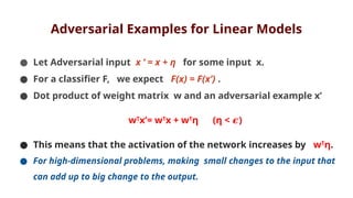
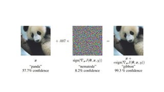
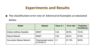
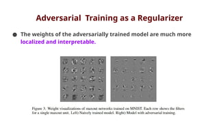
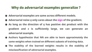
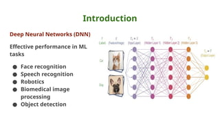
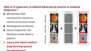
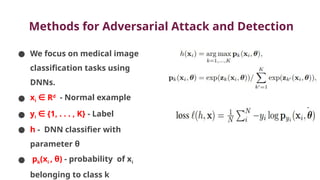
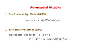
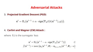
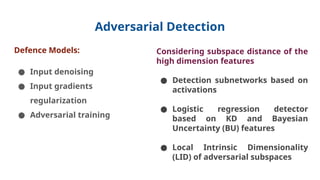
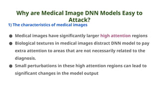
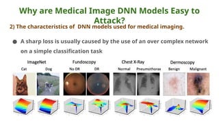
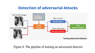
The document discusses various aspects of adversarial examples in machine learning, focusing on their creation, impact on neural networks, and methods for defense, including adversarial training and Gaussian mixture models for detection. It highlights the increased susceptibility of deep learning models, especially in medical image analysis, to adversarial attacks due to complex textures and overparameterization, while also introducing techniques to maintain privacy through differential privacy approaches. The findings indicate that adversarial attacks can be easily generated and detected, raising concerns about the robustness of models used in critical applications like medical diagnostics.

1. MANE POOJA
ROLL No. :M190442EC
SIGNAL PROCESSING
Adversarial Examples and Privacy Preserving
Schemes
Guided by
Dr. Deepthi P.P
NIT CALICUT

2. Case Studies:
1. Explaining and Harnessing Adversarial Examples
2. Robust Detection of Adversarial Attacks by Modeling the Intrinsic
Properties of Deep Neural Networks
3. Understanding Adversarial Attacks on Deep Learning Based Medical
Image Analysis Systems
4. Preserving Privacy in Convolutional Neural Network: An -tuple
𝛜
Differential Privacy Approach
5. TransNet: Training Privacy-Preserving Neural Network over
Transformed Layer

3. Explaining and Harnessing Adversarial
Examples

4. Introduction
Adversarial Example/ Adversarial Attack:
● Slightly shifted or modified version of an original image
● Adversarial examples are inputs formed by applying small
perturbations to examples from the dataset, such that the
perturbed input results in the model outputting an incorrect
answer with high confidence.

5. A
D
V
E
R
S
A
R
I
A
L
A
T
T
A
C
K

6. Motivation
● Machine Learning models can misclassify adversarial example.
● Adversarial examples are not specific to a particular type of NN
architecture.
● Exact same adversarial examples can be misclassified by different
NN architectures trained on different datasets.
● This practically means that the models are not learning the true
underlying properties of the data.

7. Motivation
Cause of Adversarial Examples :
● Non-linearity of neural networks
● Insufficient regularisation
● Insufficient model averaging

8. Important Takeaways
● We don’t need to consider the non-linearity of neural networks.
● Adversarial examples can be created by exploiting the linear
behavior in high dimensional spaces.
● It introduces a faster method to generate adversarial examples,
called Fast Gradient Sign Method.
● The paper also shows that adversarial training can be used as a
regularisation technique.

9. Adversarial Examples for Linear Models
● Let Adversarial input x ’ = x + η for some input x.
● For a classifier F, we expect F(x) = F(x’) .
● Dot product of weight matrix w and an adversarial example x’
wT
x’= wT
x + wT
η (η < )
𝝐
● This means that the activation of the network increases by wT
η.
● For high-dimensional problems, making small changes to the input that
can add up to big change to the output.

10. Fast Gradient Sign Method (FGSM):
● Method for generating Adversarial Examples.
● A simple neural network with x as input, y as target, 𝜃 as parameters
of the network has J(𝜃 , x, y) as the cost function.
● To obtain the optimal max norm constrained perturbation η, we can
linearize the cost function at 𝜃 and get
η = ϵ sign( ₓ J(
∇ 𝜃 , x, y))

12. A simple example for how such adversarial examples are
generated :
● Consider the 3’s and 7’s from MNIST dataset.
● Simple logistic regression model to do binary classification.
● The model has an error rate of 1.6% on dataset in (c).
● But on (d), the error rate is 99%.

13. Experiments and Results
● The classification error rate of Adversarial Examples as tabulated
below.

14. Adversarial Training as a Regularizer
● What actually adversarial Training is?
● Data augmentation is a very popular technique for regularization.
● Adding adversarial examples as another form of data augmentation.
● Though such translations are unlikely to occur in the real world, the
model will get exposed to its own flaws.

15. Adversarial Training as a Regularizer
● Adversarial objective function based on the Fast Gradient Sign
Method.
J(𝜃 , x, y) = α J(𝜃 , x, y) + (1-α) J(𝜃 , x + ϵ sign( ₓ J(
∇ 𝜃 , x, y)) here α = 0.5
● The error rate of the maxout network reduced from 0.94% to 0.84%
for the entire test set.
● The error rate for adversarial examples was 89.4%. With adversarial
training, this reduced to 17.9%.
● The confidence of model , misclassifying adversarial examples is still

16. Adversarial Training as a Regularizer
● The weights of the adversarially trained model are much more
localized and interpretable.

17. Why do adversarial examples generalize ?
● Adversarial examples are same across different models.
● Adversarial noise η only cares about the sign of the gradient.
● As long as the direction of η has positive dot product with the
gradient and ϵ is sufficiently large, we can generate an
adversarial example.
● Authors hypothesize that NN are able to learn approximately the
same weights when trained on different subsets of training data.
● The stability of the learned weights results in the stability of
misclassification of adversarial examples.

18. Conclusion
● The existence of adversarial examples our models truly
understand the tasks we have asked them to perform.
● Instead, their linear responses are overly confident, and
these confident predictions are often highly incorrect.

19. Robust Detection of Adversarial Attacks by
Modeling
the Intrinsic Properties of Deep Neural
Networks
paper-2

20. Introduction
Deep Neural Networks (DNN)
Effective performance in ML
tasks
● Face recognition
● Speech recognition
● Robotics
● Biomedical image
processing
● Object detection

21. Weakness of DNN classifiers
White box attack
● The attacker knows the detailed information about the model
● Model architecture, parameters, and class probabilities
Black box attack
● The attacker does not know the information about the target
model
● Architecture and parameters of a DNN are unknown to the
attackers

22. Introduction
● DNN classifiers are vulnerable to adversarial perturbations.
● We present an unsupervised learning approach to detect
adversarial inputs.
● Here we try to capture the intrinsic properties of a DNN
classifier and use them to detect adversarial inputs.

23. Attempts to defend Adversarial Attacks
Adversarial example detection : It takes the hidden states of a DNN as
input to tell if an input is adversarial. Suffers from attacks unseen
during the training procedure.
Distillation method : It reduces the magnitude of gradients during
training, to make the trained model more robust to input perturbations.
Still highly vulnerable to attacks.
Adversarial training : It focuses more on defending black-box attacks,
and usually does not consider white-box attacks

24. Related Work
Generate Adversarial Attacks
● Fast Gradient Sign Method (FGSM) : ρ = · sign( J(θ, x, l))
𝝐 ∇
● Basic Iterative Method (BIM) : x i+1
adv
= clip𝝐 {x i
adv
+ α · sign( J(θ, x
∇ i
adv
, l))}
x i+1
adv
= project𝝐{ x i
adv
+ α J(θ, x
∇ i
adv
, l) }
|| J(θ, x
∇ i
adv
, l)||2

25. Related Work
Detection Methods :
● DNN with a subnetwork : The subnetwork connects each layer of
the DNN and is trained separately using a dataset containing
both natural samples and adversarial samples generated by
known attack methods.
● SafetyNet that trains a Support Vector Machine : To detect the
boundary between natural and perturbed data in the space of
the quantified features from a DNN.

26. Related Works
Defense-GAN (Generative Adversarial Network) :
● Defense-GAN trains a generative model to model the distribution of
natural inputs.
● To detect adversarial inputs, Defense-GAN projects an input onto the
range of the GAN generator by a Gradient Descent (GD) procedure to
minimize the Wasserstein distance between the input and the
sample generated by the GAN generator.
● An input will be detected as an attack if the minimal Wasserstein
distance larger than a threshold.

27. Proposed Method : I-Defender
● Considers outputs of hidden neurons of a DNN classifier can be
much simpler.
● The dimensions of the hidden state spaces are often much lower
than that of the input space, which makes much easier to model
than the input distribution.
● I-defender uses the IHSDs of a classifier to reject adversarial
inputs as they tend to produce hidden states lying in the low
density regions of the IHSD.
● Can be easily attached to any model that produce internal

28. Proposed Method : I-Defender
● I-defender uses Gaussian Mixture Model (GMM) to approximate the
IHSD of each class as the following:
● H(x) : hidden state of an input x the c-th class,
∈
● θ : parameters
● µck : mean of k-th Gaussian component of the c-th class
● Σck : covariance matrix of k-th Gaussian component of the c-th
class.

29. Proposed Method : I-Defender
● After training the DNN classifier, we feed all training samples
into it and collect the corresponding hidden states for training a
GMM for each class using the EM algorithm.
Reject(x, c) = p(H(x)|θ, c) < THc

30. Experiments
● Datasets : MNIST, F-MNIST, CIFAR-10
● Attack methods : l∞ norm Iterative, l
− 2 norm Iterative, FGSM, and
−
DeepFool.
● Number of iterations : 10

31. Results
Black-box Attack : Attackers know nothing about the defense strategy .
Semi White-box Attack : Attackers know all details of the DNN classifier,
but have no knowledge of its defense strategy.
Gray-box Attack : Attackers know the architecture of the DNN classifier
and its defense strategy, but have no knowledge of their parameters.

32. Black-Box attack
● We first compared I-defender with Defense-GAN under the FGSM
attack.
● Attackers generated adversarial examples using model E, and used
them to attack model F

33. Black-Box attack

34. Black-Box attack

35. Semi White-box Attack
● CIFAR-10 dataset
● We trained a 34-layer wide residual network with k = 8 as the
classifier.
● We compared I-defender with two supervised detection methods,
SafetyNet and Subnetwork.

36. Conclusion
● Reliable.
● Do not need any knowledge about attack methods.
● Defend against various of black-box and gray-box attacks.
● Achieves state-of-the-art performance among unsupervised
methods
● Can be incorporated into any DNN-based classifiers
● Depending on applications, one can replace GMM with other more
appropriate models to approximate hidden state distributions.
● It can be directly applied to other modalities (such as text).

37. Understanding Adversarial Attacks on Deep
Learning Based Medical Image Analysis
Systems
paper-3

38. Deep learning based Medical Image Analysis
Medical Image Classification
● Diabetic retinopathy from
retinal fundoscopy
● Lung diseases from chest X-ray
● Skin cancer from dermoscopic
photographs
Segmentation of organs or lesions
● Quantitatively measure the
organs, such as vessels and
kidneys
Registration
● Spatially align medical images
from different modalities
● Exploit the local similarity
between eg: CT and MRI

39. Why is it important to defend Adversarial attacks in medical
diagnosis ?
● Manipulate their
examination reports to
commit Insurance Fraud.
● Misdiagnosis of disease.
● Severe impact for the
decisions made about a
patient.
➔ secure and robust medical
deep learning systems

40. Main contributions
● To find adversarial attacks on medical images.
● Less perturbation is required to generate a successful attack on
medical images.
● Higher vulnerability of medical image due to
➔ Complex Biological Textures and High gradient regions.
➔ DNN designed for Medical image processing can be
overparameterized.
● Medical image adversarial attacks can also be easily detected as
adversarial attacks result in perturbations to widespread regions

41. Deep learning based Medical Image Analysis

42. Methods for Adversarial Attack and Detection
● We focus on medical image
classification tasks using
DNNs.
● xi R
∈ d
- Normal example
● yi {1, . . . , K}
∈ - Label
● h - DNN classifier with
parameter θ
● pk(xi , θ) - probability of xi
belonging to class k

43. Adversarial Attacks
● Attacking method is to maximize the classification error of the DNN
model
Targeted attack
The target model to recognize the adversarial example as a particular
intended class
𝑥∗ : 𝑎𝑟𝑔𝑚𝑖𝑛𝑥∗ ( , ) s.t. F (x ) =
𝐿 𝑥 𝑥∗ ∗ 𝑦∗
Untargeted attack
The target model to recognize the adversarial example as a class other
than the original class.

44. Adversarial Attacks
1. Fast Gradient Sign Method (FGSM) :
2. Basic Iterative Method (BIM):
α : step size and set to /T α <
𝟄 ≤ 𝟄

45. Adversarial Attacks
3. Projected Gradient Descent (PGD)
4. Carlini and Wagner (CW) Attack :
where f(·) is the surrogate loss

46. Adversarial Detection
Defence Models:
● Input denoising
● Input gradients
regularization
● Adversarial training
Considering subspace distance of the
high dimension features
● Detection subnetworks based on
activations
● Logistic regression detector
based on KD and Bayesian
Uncertainty (BU) features
● Local Intrinsic Dimensionality
(LID) of adversarial subspaces

47. Adversarial Detection
Kernel Density (KD)
Local Intrinsic Dimensionality (LID)

48. Datasets Used
1) Diabetic retinopathy (eye disease) from Retinal fundoscopy
2) Thorax diseases from Chest X-rays
3) Melanoma (skin cancer) from Dermoscopic Images

49. Datasets

50. Datasets
For Model Training and Attacking experiments, we need two subsets of
data
1) subset Train for pre-training the DNN model
2) subset Test for evaluating the DNN model and generating adversarial
attacks.
In the detection experiments, we further split the Test data into two
parts

51. DNN Models
● We use ImageNet and ResNet-50 as the base network.
● Top layer is replaced by a new dense layer of 128 neurons, followed by a
dropout layer of rate 0.2, and K neuron dense layer for classification.
● The networks are trained for 300 epochs using stochastic gradient
descent (SGD) optimizer with initial learning rate 10 4
−
, momentum 0.9.
● All images are center-cropped to the size 224×224×3 and normalized to
the range of [ 1, 1].
−
● Simple data augmentations including random rotations, width/height
shift and horizontal flip are used.

52. Understanding Adversarial Attacks on Medical Image
DNNs
➔ All 4 types of attacks are
applied on both the AdvTrain
and AdvTest subsets of
images.
➔ The perturbation steps for BIM,
PGD and CW are set to 40, 20
and 20 respectively.
➔ Step size are set to /40, /10
𝝐 𝝐
and /10
𝝐 accordingly.

53. Attack Results
● The attack difficulty is measured by from
𝝐 0.2/255 to 5/255.
● Model accuracy drops drastically when adversarial perturbation
increases.
● Strong attacks including BIM, PGD and CW, only require a small
maximum perturbation < 1.0/255
𝝐 to generally succeed.
● Model accuracy decreases as the number of classes increases.

54. Why are Medical Image DNN Models Easy to
Attack?
1) The characteristics of medical images
● Medical images have significantly larger high attention regions
● Biological textures in medical images distract DNN model to pay
extra attention to areas that are not necessarily related to the
diagnosis.
● Small perturbations in these high attention regions can lead to
significant changes in the model output

55. Why are Medical Image DNN Models Easy to
Attack?
2) The characteristics of DNN models used for medical imaging.
● A sharp loss is usually caused by the use of an over complex network
on a simple classification task

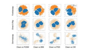
56. Detection of Medical Image Attacks
Adversarial detection experiments
on 2-class datasets
● KD
● LID
● Qfeat-quantized deep features
● Dfeat- Deep features
● All detection features are extracted
in mini-batches of size 100
● The detection features are then
normalized to [0,1].
● Logistic regression classifier as the
detector for KD and LID.
● Random forests classifier as the
detector for the deep features.
● SVM classifier for quantized deep

57. Detection of adversarial Attacks

58. Detection Results:
● KD-based detectors, achieve an AUC of above 99% against all attacks
across all three datasets.
● Deep features alone can deliver very robust detection performance
against all attacks above 98%.
● Quantized deep features also achieve good detection performance.
● This indicates that the adversarial features may be fundamentally
different from that of normal features.

59. Why are Adversarial Attacks on Medical Images Easy
to Detect?
● Adversarial features are almost linearly separable
● Compared to natural images, adversarial perturbations tend to
cause more significant distortions on medical images .
● Deep representations of natural images cover a large area of the
representation map
● Deep representations of medical images are very simple and cover a
small region of the representation map

61. Conclusion
● Adversarial attacks on medical images are much easier to generate.
● Adversarial examples are also much easier to detect.
● Can also work with UNSEEN attacks adversarial attacks tend to
attack a widespread area outside the pathological regions

62. Preserving Privacy in Convolutional Neural
Network: An -tuple Differential Privacy Approach
𝛜
paper-4

63. Introduction:
Convolutional Neural Network
● Features extraction,
● Data predictions,
● Data classification,
● Computer visioning
CNNs made available over cloud
system or networks for clients who
want to train their data but do not
have the computational resources
to do so.
Model Inversion are attacks that
expose sensitive information using
an ML system.
CNN model does memorize random
data during learning phase-
(privacy violation)

64. Introduction:
Differential privacy :
● This technique makes use of Laplace mechanism, relies on privacy
budget parameter 𝜖 to generate noise used to enact privacy,
● Degrades accuracy.
● Neurons within CNN model do not have equal impact factor.
● Differential privacy initially estimates the impact factor of each
neuron in the layers of our model and on that basis generate a tuple
of for distinct neurons.
𝜖
● The -tuple is then used to preserve privacy of our CNN model
𝜖

65. Background
● CNN: It is based on the convolution of images and extraction features
based on filters that are learned by the network during training phase
● Includes: convolution layer, activation layer, pooling layer, and fully-
connected layer

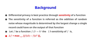
66. Background
Differential Privacy (DF) :
● Differential privacy (DF) is a concept that reduces the likelihood of
identifying a record within a large database
● DF basically relies on exponential or Laplace mechanism to perturb
data.
● Pr[ℛ(𝐷1) ]
∈ ≤
𝑆 𝑒𝜖
Pr[ℛ(𝐷2) ]
∈ 𝑆 : level of privacy budget
𝜖
● 𝜖 is inversely proportional to privacy protection

67. Background
● Differential privacy is best practice through sensitivity of a function
● The sensitivity of a function is referred as the addition of random
noise whose magnitude is determined by the largest change a single
record could have on the output of that function
● Let be a function : ℝ
𝑓 𝑓 𝐷 → 𝑑
the 1-sensitivity of is,
𝐿 𝑓
● ∆𝑓 = max , ′
𝑑 𝑑 ‖ ( ) ( ′ )‖
𝑓 𝑑 − 𝑓 𝑑 1

68. Proposed method
𝜖-tuple differential privacy approach for preserving privacy in CNN.
● We achieve by combining a differential privacy (DP) approach and
neuron’s impact factor estimator (IFE)
Neuron Impact Factor Estimator(IFE)
● IFE is to avoid excess noise injection into the CNN network which
degrades classification accuracy.

70. 𝜖-tuple Fabrication and Perturbation process
● Impact factor estimator ,
where is total number of
𝑞
neuron in the hidden layer l
𝜔
● A tuple of impact factor
estimate along with an ϵ
bound are used to
𝐸
fabricate 𝜖 u le
𝑡 𝑝 .

71. 𝜖-tuple Fabrication and Perturbation process
● We compute our perturbation process by setting the sensitive
maximum training data tuple ,
𝑋
● Perturb loss function

72. Experimental Results
Experiments were conducted in 2 phases
1. pre-training which captures the neurons impact factor
2. Training which classifies the dataset.
Datasets:
3. MNIST dataset which consist of 60,000 training handwritten digits
examples
4. Emotion recognition dataset with 4,178 training samples were used

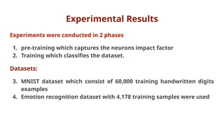
73. Emotion Recognition Dataset
● Emotion dataset has 7 classes (i.e. anger, disgust, fear, happy, sad,
surprise, neutral)
● In the non-private model 83.7% test accuracy was reached.
● We introduce moderate noise into CNN model through our bound
𝜖
E as: E = [0.5 5], 82.8% testing prediction accuracy was observed.
∶
● We increase the noise by setting E = [0.1 1], the accuracy was at
∶
81.5%.
● The results indicate a close accuracy between private and the non-
private model.

74. MNIST Dataset
● MNIST is a well-known dataset with training accuracy of
99.7% .
● We set our bound E to: E = [0.5 5] for moderate noise,
𝜖 ∶
and our model achieved an accuracy of 98.6%,
● When we introduced much noise as E = [0.1 1], our CNN
∶
model recorded an accuracy of 98.1%.

75. Conclusion
● This approach leverage on neuron impact factor estimation to
determine quantity of Laplace noise to be injected into distinct
neuron input in the network.
● Extensive experiment were carried out on two large datasets.
● The result shows a big reduction in significant accuracy disparity
between non-privacy preserving and privacy preserving CNN model.