The document is a course sampler for a short course on engineering probability and visualization techniques using MATLAB, led by Dr. Ralph E. Morganstern. It covers fundamental probability concepts, including sample space, event space, and various representations such as matrix and tree diagrams, along with the application of DeMorgan's laws and counting principles. The Applied Technology Institute offers tailored training programs aimed at enhancing technical professionals' skills in a competitive marketplace.

1. Course Sampler From ATI Professional Development Short Course
Fundamentals of Engineering Probability
Visualization Techniques & MatLab Case Studies
Instructor:
Dr. Ralph E. Morganstern
ATI Course Schedule: http://www.ATIcourses.com/schedule.htm
ATI's Engineering Probability: http://www.aticourses.com/Fundamentals_of_Engineering_Probability.htm

2. www.ATIcourses.com
Boost Your Skills 349 Berkshire Drive
Riva, Maryland 21140
with On-Site Courses Telephone 1-888-501-2100 / (410) 965-8805
Tailored to Your Needs
Fax (410) 956-5785
Email: ATI@ATIcourses.com
The Applied Technology Institute specializes in training programs for technical professionals. Our courses keep you
current in the state-of-the-art technology that is essential to keep your company on the cutting edge in today’s highly
competitive marketplace. Since 1984, ATI has earned the trust of training departments nationwide, and has presented
on-site training at the major Navy, Air Force and NASA centers, and for a large number of contractors. Our training
increases effectiveness and productivity. Learn from the proven best.
For a Free On-Site Quote Visit Us At: http://www.ATIcourses.com/free_onsite_quote.asp
For Our Current Public Course Schedule Go To: http://www.ATIcourses.com/schedule.htm

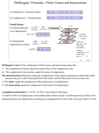
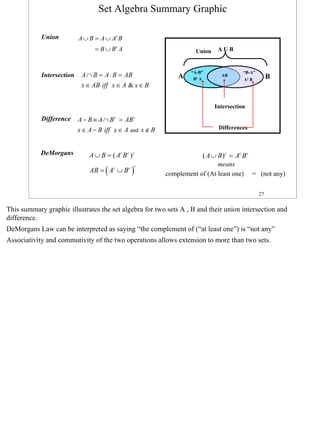
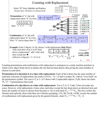
3. Fundamental Probability Concepts
• Probabilistic Interpretation of Random Experiments (P)
– Outcomes: sample space
– Events: collection of outcomes (set theoretic)
– Probability Measure: assign number “probability” P ε [0,1] to event
• Dfn#1-Sample Space (S): Fine-grained enumeration (atomic - parameters)
– List all possible outcomes of a random experiment
– ME - Mutually exclusive - Disjoint “atomic”
– CE - Collectively exhaustive - Covers all outcomes
• Dfn#2- Event Space (E): Coarse-grained enumeration (re-group into sets)
– ME & CE List of Events
S (all outcomes)
Atomic Outcomes
Events: A,B,C ME but not CE A D
(Disjoint by dfn)
Events: A,B,C ,D both ME & CE
C
B
14 INDEX
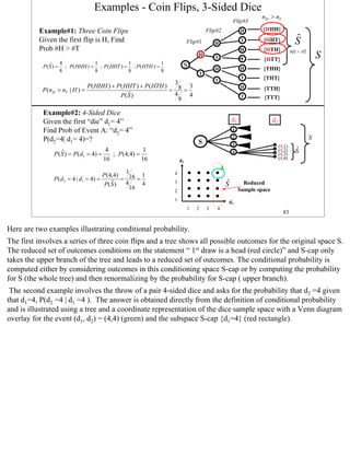
Discrete parameters uniquely define the coordinates of the Sample Space (S) and the collection of all
parameter coordinate values defines all the atomic outcomes. As such atomic outcomes are mutually
exclusive (ME) and collectively exhaustive (CE) and constitute a fundamental representation of the Sample
Space S.
By taking ranges of the parameters such as A, B, C, and D, one can define a more useful Event Space which
should consist of ME and CE events which cover all outcomes in S without overlap as shown in the figure.
14

4. Fair Dice Event Space Representations
d2
• Coordinate Representation: 6
– Pair 6-sided dice 5
A: d1=3, d2 =arb.
4
– S={(d1,d2): d1,d2 = 1,2,…,6} 3
2 C: d1=d2
– 36 Outcomes Ordered pairs 1
d1
1 2 3 4 5 6
B: d1+d =7
• Matrix Representation: 1  [1 2 3 4 5 6]  (1,1) (1,2) (1,3) (1,4) (1,5) (1,2 ) 
6
  (2,1) (2,2) (2,3) (2,4) (2,5) (2,6)
– Cartesian Product: 2  
3
 
= (3,1)

(3,2) (3,3) (3,4) (3,5) (3,6)

– {d1} x {d2} = d1 d2T 4 (4,1) (4,2) (4,3) (4,4) (4,5) (4,6)
  (5,1) (5,2) (5,3) (5,4) (5,5) (5,6)
5  
  (6,1)
 (6,2) (6,3) (6,4) (6,5) (6,6) 
6
• Tree Representation: d2
d1 (1,1)
(1,2)
1 (1,3) 36 Outcomes
(1,4) Ordered Pairs
2 (1,5)
3 (1,6)
• Polynomial Generator for Sum Start
4
2 Dice 5 (6,1)
(6,2)
( x1 + x 2 + x3 + x 4 + x5 + x 6 ) 2 = 1x 2 + 2 x3 + 3 x 4 + 4 x5 + 5 x 6 + 6 x 7 6 (6,3)
(6,4)
Exponents represent + 5 x8 + 4 x9 + 3 x10 + 2 x11 + 1x12 (6,5)
(6,6)
6-sided die face numbers Exponents represent pair sums
Coefficients represent #ways 16
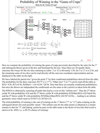
It is helpful to have simple visual representations of Sample and Event Spaces
For a pair of 6-sided dice, coordinate, matrix, and tree representations are all useful representations. Also
the polynomial generator for the sum of a pair of 6-sided dice immediately gives probabilities for each sum.
Squaring the polynomial (x1+x2+x3+x4+x5 +x6)2 yields a generator polynomial whose exponents represent
all possible sums for a pair of 6-sided dice S={2,3,4,5,6,7,8,9,10,11,12}and whose coefficients C=
{1,2,3,4,5,6,5,4,3,2,1} represent the number of ways each sum can occur. Dividing by the coefficients C by
the total #outcomes 62 = 36 yields the probability “distribution” for the pair of dice.
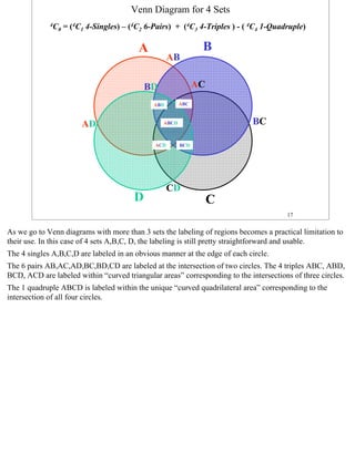
Venn diagrams for two or three events are useful; for example, the coordinate representation in the top
figure can be used to visualize the following events
A: {d1 = 3 and d2 = arbitrary, B= {d1 + d2 = 7}, and C= {d1 = d2}
Once we display these two events on the coordinate diagram their intersection properties are obvious, viz.,
both A & B and A & C intersect, albeit at different points, while B & C do not intersect (no point
corresponding to sum=7 and equal dice values). More than three intersecting sets, become problematic for
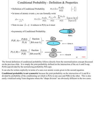
Venn diagrams as the advantage of visualization is muddled somewhat by the increasing number of
overlapping regions in theses cases (see next two slides).
16

5. Venn Diagram for 4 Sets
4C = (4C1 4-Singles) – (4C2 6-Pairs) + (4C3 4-Triples ) - ( 4C4 1-Quadruple)
0
A B
AB
BD AC
ABD ABC
AD ABCD BC
ACD BCD
CD
D C
17
As we go to Venn diagrams with more than 3 sets the labeling of regions becomes a practical limitation to
their use. In this case of 4 sets A,B,C, D, the labeling is still pretty straightforward and usable.
The 4 singles A,B,C,D are labeled in an obvious manner at the edge of each circle.
The 6 pairs AB,AC,AD,BC,BD,CD are labeled at the intersection of two circles. The 4 triples ABC, ABD,
BCD, ACD are labeled within “curved triangular areas” corresponding to the intersections of three circles.
The 1 quadruple ABCD is labeled within the unique “curved quadrilateral area” corresponding to the
intersection of all four circles.
17

6. Trivial Computation of Probabilities of Events
sum = d1 + d2
d2
Ex#1 Pair of Dice E1
S={(d1,d2): d1,d2 = 1,2,…,6} 6
12
5 11 E2
10
E1={(d1,d2): d1+d2 ¥ 10} 4 9
8
P(E1)=6/36=1/6 3 7
6
2 5
E2={(d1,d2): d1+ d2 = 7} 4
P(E2)=6/36=1/6 1 3
2 d1
1 2 3 4 5 6
Ex#2 Two Spins on Calibrated Wheel
S={(s1,s2): s1,s2 ε [0,1]} s2
E1={(s1,s2): s1+s2 ¥ 1.5}--> P(E1) = ----- =.52/2=1/8 1
1
E1
0.5 E3
E2={(s1,s2): s2 § .25} --> P(E2)=1(.25)/1=.25
E2
0 s1
E3={(s1,s2): s1= .85; s2= .35}--> P(E3)=0/1=0 0 0.5 1
20
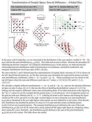
For equally likely atomic events the probability of any outcome Event is easily computed as the (#atomic
outcomes in Event)/(total # outcomes). For a pair of dice, the total # of outcomes is 6*6=36 and hence
simple counting of the # points in E /36 yields P(E), etc.
Two spins on a calibrated wheel [0, 1) can be represented by the unit square in the (s1 , s2)-plane and an
analogous calculation can be performed to obtain the probability for the event E by dividing the area
covered by the event by the area of the event space (“1”): P(E)= area(E)/ 1.
20

7. DeMorgans’ Formulas - Finite Unions and Intersections
i) Compl(Union) = Intersec(Compls): ( E1 ∪ E2 ∪
c
∪ En ) c = E1 ∩ E2 ∩
c
∩ En
c
c c c
ii) Compl(Intersec) = Union(Compls): ( E1 ∩ E2 ∩ ∩ En ) c = E1 ∪ E2 ∪ ∪ En
Useful Forms:
A∪ B
i’) Union expressed ( A ∪ B) c = Ac B c
Visualization
Compl(Union) Intersec(Compl) ( A ∪ B)c
as an Intersection
(( A ∪ B) )
c c
= A ∪ B = ( Ac B c ) c A Ac Intersect
grey areas
B Bc Ac & B c
ii’) Intersection ( AB) c = Ac ∪ B c Ac B c Yields one
Union(Compl) grey area Ac B c
expressed as a Union Compl(Intersec)
with A and
B excluded
(( AB) )
c c
(
= AB = Ac ∪ B c )c
Taking its
complement ( Ac B c )c
yields white
area, i.e., A ∪ B
24 INDEX
DeMorgan’s Laws for the complement of finite unions and intersections states that
i) The complement of unions equals the intersections of the complements, and
ii) The complement of intersections equals the union of complements
The alternate forms obtained by taking the complements of the original equations are often more useful
because they give a direct decomposition of the union and the intersection of two or more sets
i’) The union equals the complement of the (intersection of complements)
ii’) The intersection equals the complement of the (union of complements)
A graphical construction of A U B = (Ac Bc)c is also shown in the figure..
Ac and Bc are the two shaded areas in the middle planes which exclude A and B respectively (white) ovals
Intersecting these two shaded areas and taking the complement leaves the white oval areas which is A U B
24

8. Set Algebra Summary Graphic
Union A ∪ B = A ∪ Ac B
= B ∪ Bc A Union AUB
“A-B” “B-A”
Intersection A ∩ B = A ⋅ B = AB A Bc A
AB B
Ac B
x ∈ AB iff x ∈ A & x ∈ B
Intersection
Difference A − B ≡ A ∩ B c = AB c
x ∈ A − B iff x ∈ A and x ∉ B Differences
DeMorgans A ∪ B = ( Ac B c )c ( A ∪ B )c = Ac B c
means
( )
c
AB = Ac ∪ B c complement of (At least one) = (not any)
27
This summary graphic illustrates the set algebra for two sets A , B and their union intersection and
difference.
DeMorgans Law can be interpreted as saying “the complement of (“at least one”) is “not any”
Associativity and commutivity of the two operations allows extension to more than two sets.
27

9. Basic Counting Principles
Principle #0: Take Case n=3-4; generalize to n Binomial Expansion: (a+b)3 (a+b)n
Repetitions Allowed
Principle #1: Product Rule for Sub-experiments: 6- Bins
= 263 ⋅103
m Num Suit
Licenses
⋅ nm = ∏ nk
26 26 26 10 10 10
n = n1 ⋅ n2
H
1 D
S
C
H
5
16- Bins
k =1 Start 2 D
Binary
S
2
216 = 65,536
C
H
13 D
2 2 2 2 ... 2
Generate “tree” of outcomes
S
C Digits
#ways: 13 * 4 = 52
No Repetitions
Principle #2: Perm n distinguish-obj take k k=n Arrange 11 Travel 5 Cooking 4 Garden
All Books
n! “Fill k-bins” 11! 5! 4!
n
Pk = (n) k = 3! Permute Groups
(n − k )! k<n 11 Travel Books
in 5 bins 11| 10| 9 |8 |7
Principle #3:Perm n-obj take n with r - Arrange 4!
groups of indistinguishable objects Letters
“TOOL” = 12
2!⋅1!⋅1!
hable
 # Distinguis n! 10!
 Sequences  = n !⋅n !⋅ ⋅ n !
  r − groups {4”r”, 3”s”, 2”o”, 1 “t”}
4!⋅3!⋅2!⋅1!
= 12,600
  1 2 r
Principle #4: Combination of n-objects take k Committee of 4 22! 22!
C4 =
22
= = 7315
from 22 people (22 − 4)!4! 18!4!
n n!
n
Ck =   =
 k  k ! ( n − k )! k ≤ n Order not
  Committee of 3 {2M, 1F} 6⋅5
important!
from {6M, 3F}
6
C2 ⋅3 C1 = ⋅ 3 = 45
2!
= Principle #3 with {taken , not taken} not counted 28 INDEX
Outcomes must be distinguished by labels. They are characterized by either i) distinct orderings or ii)
distinct groupings. A grouping consists of objects with distinct labels; changing order within a group is not
a new group, but is a new permutation. The four basic counting principles for groups of distinguishable
objects are summarized and examples of each are displayed in the table.
Principle#0: This is practical advice to solve a problem with n= 2,3,4 objects first and then generalize the
“solution pattern” to general n.
Principle#1: This product rule is best understood in terms of the multiplicative nature of outcomes as we
“branch out” on a tree. For a a single draw from a deck of cards there are 13 “number” branches and, in
turn, each of these has 4 “suit” branches yielding 13*4 =52 distinguishable cards or outcomes.
Principle#2: Permutation (ordering) of n objects take k at a time is best understood by setting up “k-
containers” putting one of “n” in the first, one of “n-1” , ... and finally one of “n-k+1” in the kth container.
The total #ways is obtained by the product rule as n*(n-1)*...*(n-k+1) = n!/(n-k)!
Principle#3: Permutation of all ”n” objects consisting of “r “ groups of indistinguishable objects {3 t , 4
s 5 u}. If all objects were distinguishable then the result would be n! permutations; however permutations
within the r groups does not create new outcomes and therefore we divide by factorials of the numbers in
each group to obtain n!/(n1! n2! ... nr!)
Principle#4: Combination of n objects take k is related to Principles#2, #3. There are n! permutations;
ignoring permutations within r= 2 groups {“taken” , “not taken”} yields n!/(n! (n-k)!)
28

10. Counting with Replacement
Refills Drop Down
Select “B” from Alphabet and Replace A
A
B
B ... Y
Y
Z
Z
Always have 26 letters to choose from A
A
B
B
Y
Y
Z
Z
23 =8 distinct 4 distinct
Permutation of “n” obj with (# drws)
orderings groupings
replacement taken “k” at a time
n
Pk = # replaceable
objects = nk A {AAA} 3 “A”
B {AAB} 2 “A”& 1”B”
A
n n n n n…n A {ABA} 2 “A”& 1”B”
A B B {ABB} 2 “B”& 1”A”
Bin# 1 2 3 …k S A A {BAA} 2 “A”& 1”B”
B
n=2 , k=3 B B {BAB} 2 “B”& 1”A”
A {BBA} 2 “B”& 1”A”
B {BBB} 3 “B”
Combination of “n” obj with
replacement taken “k” at a time
effective # objects
 n + k − 1  n + k − 1
n
Ck =
/ n + (k-1)
= n + k −1
Ck =  = 
Note: “k” can be larger than “n”
(draw k)  k   n −1 
Example: From 2 objects {A, B} choose 3 with replacement (Only Way!)
After each draw of an A or B “drop 4 Outcomes
down a replacement” add 1 after each A B A/B A/B
{AAA},{BBB}
draw except last 4! {ABB},{AAB}
(effective # objects) = 2 +(3-1)=4
2
C3 = 2+3−1C3 = 4C3 =
/ =4
3! 1!
41 INDEX
Counting permutations and combinations with replacement is analogous to a candy machine purchase in
which a new object drops down to replace the one that has been drawn, thus giving the same number of
choices in each draw.
Permutation of n obj taken k at a time with replacement: Each of the k draws has the same number of
outcomes n because of replacement, the result is n*n*n... *n = nk and is written nPk with an “over-slash” on
the permutation symbol. The case n=2, k=3 of 3 draws with 2 replaceable objects {A,B} shows the slash-
2
P3 =23 = 8 permutations that result.
Combination of n obj taken k at a time with replacement: For n=2, k=3, 2 take 3 does not make any
sense. However, with replacement, it does since each draw except the last drops down an identical item and
hence the number of items to choose from becomes n +(k-1) and slash-nCk = n+(k-1)Ck. The tree verifies this
formula and explicitly shows that there are 4 distinct groupings {3A, 3B, 2A1B, 1A2B} exactly the number
of combinations with replacement given by the general formula slash-2C3 = 2+(3-1)C3 = 4C3 =4
41

11. II) Fundamentals of Probability
1. Axioms
2. Formulations: Classical, Frequentist, Bayesian, Ad Hoc
3. Adding Probabilities: Inclusion / Exclusion, CE & ME
4. Application of Venn Diagrams & Trees
5. Conditional Probability & Bayes’ “Inverse Probability”
6. Independent versus Disjoint Events
7. System Reliability Analysis
47
As a theory, Probability is based on a small set of axioms which set forth fundamental properties of
construction.
In practice, probability may be formulated theoretically, experimentally, or subjectively, but must always
obey the basic Axioms.
Evaluating probabilities for events, is naturally developed in terms of their unions and intersections using
Venn Diagrams, Trees and Inclusion/Exclusion techniques.
Conditional probabilities, their inverses (Bayes’ theorem), and the dependence between two or more events
flow naturally from the basic axioms of probability.
System reliability analysis utilizes all these fundamental concepts
47

12. Inclusion / Exclusion Ideas
ME Events A,B - Disjoint AB= φ A B P(A∩B) = P(A) + P(B) No intersections
”Add Prob”
No intersections
Intersect: “CE, not ME” “Recast” as Disjoint Union “CE & ME”
Not Disjoint AB∫φ
A A B-A
B ∫
AB
P(A∩B) = P(A) + P(B-A) = P(A) + P(BAc)
Intersection “AB” Counted Twice!! P(A∩B) ∫ P(A) + P(B)
B = B ⋅ S = B ⋅ ( A ∪ Ac ) = BA ∪ BAc
Subtract “P(AB)” from sum; count only once
A
BAC B
P ( A ∪ B ) = P ( A) + P ( B ) − P ( AB ) AB
P( BAc ) = P( B) − P( AB)
Generalization by Induction: let D = B ∪ C
P ( A ∪ B ∪ C ) = P ( A ∪ D ) = P ( A) + P ( D) − P ( AD ) = P ( A) + P ( B ∪ C ) − P( A ⋅ ( B ∪ C ))
= P ( A) + {P ( B ) + P (C ) − P ( BC )} − {P ( AB ) + P ( AC ) − P ( ABAC )}
Inclusion /
P ( A ∪ B ∪ C ) = P ( A) + P ( B ) + P (C ) − P ( AB ) − P ( AC ) − P ( BC ) + P ( ABC ) Exclusion
add singles subtract pairs add triples
54 INDEX
It is important to realize that although probabilities are simply numbers that add, the probability of the
union of two events P(A U B) is not equal to the sum of individual probabilities for the two events P(A) +
P(B).
This is because points in this overlap region AB are counted twice; to correct for this one needs to subtract
out “once” the double counted points in the overlap yielding P(A U B) = P(A) + P(B)-P(AB).
Only in the case of non-intersection AB = φ does the simple sum of probabilities hold.
The generalization for a union of three or more sets alternates inclusion and exclusion; for A,B,C the
probability P(AUBUC) adds the singles, subtracts the doubles and adds the triple as shown.
54

13. Venn Diagram Application: Inclusion/Exclusion
Given following information find how many club
members play at least one sport T or S or B T (36) TS (22) S (28)
Club: 36 T , 28 S, 18 B
TSB
(4)
SB (9)
Let N= Total # members (unknown) TB (12)
36 28 18 B (18)
Write Probabilities as P(T) = ; P(S) = ; P(B) = ; etc.
N N N CLUB
Method 1: Subs into Formula for Union
P ( T ∪ S ∪ B) = P (T ) + P( S ) + P( B ) − P (TS ) − P(TB ) − P ( BS ) + P (TBS )
36 28 18 22 12 9 4 TS (22)
= + + − − − + T (36) STc (6)
N N N N N N N
43 18 1
= Thus 43 of “N” Club Members play 6 TSB
N at least one sport. (N is irrelevant) (4) 5
8 SB (9)
Method 2: Disjoint Union - Graphical TB (12) 1
T ∪ S ∪ B = T ∪ ST ∪ BT Sc c c
BTcSc (1)
CLUB
P(T ∪ S ∪ B) = P(T ) + P( ST c ) + P( BT c S c )
36 6 1 43
= + + =
N N N N
68 INDEX
This example illustrates the ease by which a Venn diagram can display the probabilities associated with the
various intersections of 3 sets T, S, and B.
The number of elements in each of the 7 distinct regions is easily read off the figure; they are required to
establish the total number in their union T U S U B via the inclusion/exclusion formula.
Another method of finding P(T U S U B ) is to decompose the union T U S U B into a union of disjoint sets
T* U S* U B* for which the probability is additive, i.e., P(T* U S* U B* ) = P(T*) + P(U*) + P(B*).
68

14. Matching Problem – 1
“N” men throw hats onto floor; Each man in turn randomly draws a hat
a) No Matches - Find Probability None draw own hat.
Let Event Ei = ith man chooses his own hat ; compute: P(0 − matches) = 1 − P( E1 ∪ E2 ∪ ∪ EN )
1|2|3|… | k | k+1 | … |N Hats
i1 |i2 | i3 | … | in in+1 | in+2 | in+3 | … | iN Men
Probability that
M1 & M2 &...&Mn irrespective of what
n “Ei s” choose own hats (N-n) Does not Matter
draw own hats other men draw
(Matched or Not Matched )
Total # of“n-tuple” N # perms ( N − n)!
  P( Ei1 Ei2 Ein ) = =
selections from N n Total# perms N!
 
 N  ( N − n)! N! ( N − n)! 1
Sum Joint Probabilities
∑ P( Ei1 Ei2 Ein ) =   ⋅ =
n !( N − n)! N !
=
over all “n-tuples” n −tuples
All n-tuples Eq. Likely
n N! n!
 
P (0 − Matches ) = 1 − P ( E1 ∪ E2 ∪ E3 ) = 1 −  ∑ P ( Ei1 ) − ∑ P ( Ei1 Ei2 ) + ∑ P( Ei1 Ei2 Ei3 ) = 1 − {1 − 2! + 3!} =
1 1 1
3
1− tuples pairs triples 
P(0 − matches) = 1 − P( E1 ∪ E2 ∪ ∪ EN ) = 1
−
1
+
1
−
2! 3! 4! 5!
1
+ + ( −1)
N 1
N!
 e−1
N →∞
→
b) k- Matches
Poisson with success rate λ=1/N & “time
 k! ⋅ e−1
→1
1 1 1 N −k 1 
 − + + + ( −1) 
( N − k )! 
P(k matches) =  2! 3! 4!
N→∞ intvl” t = N samples; a=λ *t =(1/N)*N =1
k!
69 INDEX
Here is an example that requires the inclusion/exclusion expansion for a large number of intersecting sets.
Since it becomes increasingly difficult to use Venn diagrams for a large number of intersecting sets, we
must use the set theoretic expansion to compute the probability. We shall spend some time on this problem
as it is very rich in probability concepts.
The problem statement is simple enough: “N men throw their hats onto the floor; each man in turn
randomly draws a hat. “
a) What is the probability that no man draws his own hat?
b) What is the probability of exactly k-matches?
Key ideas: define Event Ei = ith man selects his own hat
then take union of N sets E1 U E2 U ... U EN and
P(no-matches)=1- P(E1 U E2 U ... U EN)
The expansion of the P(E1 U E2 U ... U EN) involves addition and subtraction of P(singles), P(pairs),
P(triples), etc. ( The events Ei are CE but not ME so you cannot simply sum up the P(Ei ) for k singles to
obtain an answer to part b)) .
This slide shows a key part of the proof which establishes the very simple result that the sum over singles,
P(singles) = 1/(1!); sum over pairs is P(pairs)= 1/(2!) ; sum over triples is P(triples)=1/(3!); sum over 4-
tuples, P(4-tuples) = 1/(4!); ... sum over N-tuples, P(N-tuple) = 1/(N!).
Limit as N large approaches a Poisson Distribution with success rate for each draw λ=1/N and data length
t =N i.e., parameter a =λ t =1
69

15. Man Hat Problem n =3 Tree/Table Counting
M#1 M#2 M#3 M.E. Match
Tree#1 Drw#1
Drw#2 Drw#3 Outcomes Outcomes
M#1 M#2 M#3 #Matches
E2 1
2 3 E3 {E1 E2 E3 } triple 1 2 3 3
1/2 Br#1
1
E1 1/2 3 2 c
{E1 E2 E3 }
c
single 1 3 2 1
1/3 1 1/2
1
1
3 E3 {E1c E2 c E3 } single 2 1 3 1
E1C Br#2
Start 1/3 2 1/2 1
1
c c
{E1 E2 E3 }
c
No-match 2 3 1 0
3
1/3 1/2
3 1
1
2 c c
{E1 E2 E3 }
c
No-match 3 1 2 0 Br#3
E1C
1/2
2 E2
1
1 c
{E1 E2 E3 }
c
single 3 2 1 1
P(Ei) = 1/3 2/6 2/6
From Table: From Tree: Connection: Matches & Events
Prob[0-matches]=2/6 Prob[0-matches]=1-Pr[E1 U E2 U E3]
Prob[1-matches]=3/6 Prob[Sgls]=P[E1]=P[E2]=P[E3]=1/3
=1-{Sum[Sngls]-Sum[Dbls]+Sum[Trpls]}
Prob[2-matches]=0/6=0 Prob[Dbls] = P[E1E2]=(1/3)(1/2)=1/6 =1-{3(1/3) -3(1/6)+1(1/6)}=2/6
Prob[3-matches]=1/6 Prob[Trpls] = P[E1E2E3]=(1/3)(1/2)=1/6
Alternate Trees Yield: P[E1E3]= P[E2E3]=1/6
75
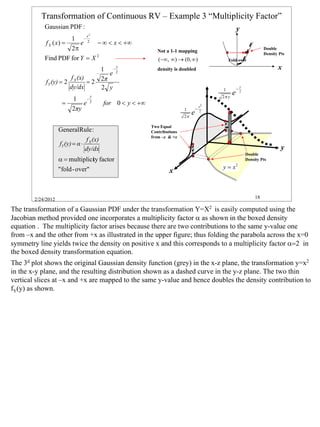
This slide shows the complete the tree and associated table for the Man - Hat problem in which n=3 men
throw their hats in the center of a room and then randomly select a hat. The drawing order is fixed as
Man#1, Man#2, Man #3, and the 1st column of nodes labeled as circled 1, 2, 3 shows the event E1 in which
the Man#1draws his own hat, and the complementary event E1c i.e., Man#1 does not draw his own hat . The
2nd column of nodes corresponds to the remaining two hats in each branch shows the event E2 in which the
Man#2 draws his own hat; note that E2 has two contributions of 1/6 summing to 1/3. Similarly, the 3rd draw
results in the event E3 in two positions shown again summing to 1/3.
The tree yields ME & CE outcomes expressed as composite states such as {E1E2E3}, {E1E2cE3c, etc., or
equivalently in terms of the number of matches in the next column. The nodal sequence in the tree can be
translated into the table on the right which is analogous to the table we used on the previous slide. The
number of matches can be counted directly from the table as shown.
The lower half of the slide compares the “ # of matches” events with the “compound events” formed from
the “Ei”s{ no-matches, singles, pairs, and triples }. The connection between these two types of events is
based on the common event “no-matches,” i.e., the inclusion/exclusion expansion of the expression [1-
P(E1U E2U E3) ] in terms of singles doubles and triples yields P(0-matches).
75

16. Conditional Probability - Definition & Properties
ˆ
P ( AS )  2
• Definition of Conditional Probability ˆ
P( A | S ) ≡ = 
ˆ
P( S )  3
• In terms of atomic events si we can formally write
ˆ ˆ
P( ∪ si S ) ∑ P( s S )
ˆ
i
(# pts in Sˆ & A)
A = ∪ si ˆ ) = P ( A S ) = si ∈ A =
si ∈ A
=
si ∈ A
P( A | S
ˆ
P( S ) ˆ
P( S ) ˆ
P( S ) (# pts in Sˆ )
ˆ
• Note in case S = S it reduces to P(A) as it must
A B
•Asymmetry of Conditional Probability BA
P(BA)
P ( BA)  fraction  BA
P ( B | A) = = =
P ( A)  BA over A 
  A Given A
Not
Symmetrical!
P( BA)  fraction  BA
P( A | B) = = =
P( B)  BA over B 
  Given B
B
82 INDEX
The formal definition of conditional probability follows directly from the renormalization concept discussed
on the previous slide. It is simply the joint probability defined on the intersection of the set A and S-cap,
P(AS-cap) divided by the normalizing probability P(S-cap).
It can also be written explicitly in terms of a sum over atomic events given in the second equation.
Conditional probability is not symmetric because the joint probability on the intersection of A and B is
divided by probability of the conditioning set which is P(A) in one case and P(B) in the other. This is also
easily visualized using Venn diagrams where the “shape division” are obviously different in the two cases.
82

17. Examples - Coin Flips, 3-Sided Dice
nH > nT
Flip#3
Example#1: Three Coin Flips Flip#2 H {HHH}
Given the first flip is H, Find Flip#1 H
T {HHT} ˆ
S
Prob #H > #T H {HTH}
H
T T {HTT}
#H > #T
S
4 1 1 1
ˆ
P ( S ) = ; P( HHH ) = ; P ( HHT ) = ; P( HTH ) = S H H {THH}
8 8 8 8
T
T
T {THT}
3
P ( HHH ) + P ( HHT ) + P ( HTH ) 3
= 8=
H {TTH}
P (nH > nT | H ) =
ˆ)
P( S 4 4 T
8 {TTT}
Example#2: 4-Sided Dice
Given the first “die” d1= 4” d1 d2
Find Prob of Event A: “d2= 4” 1
P(d2=4| d1= 4)=? 2 S
S 3 (4,1)
ˆ 4 1 4 (4,2) ˆ
S
P ( S ) = P( d1 = 4) = ; P( 4,4) = (4,3)
16 16 d2 (4,4)
A
1 4
P(4,4) 1
P (d 2 = 4 | d1 = 4) = = 16 =
ˆ
P( S ) 4 4 3 ˆ
S Reduced
16 2 Sample space
1 d1
1 2 3 4
83
Here are two examples illustrating conditional probability.
The first involves a series of three coin flips and a tree shows all possible outcomes for the original space S.
The reduced set of outcomes conditions on the statement “ 1st draw is a head (red circle)” and S-cap only
takes the upper branch of the tree and leads to a reduced set of outcomes. The conditional probability is
computed either by considering outcomes in this conditioning space S-cap or by computing the probability
for S (the whole tree) and then renormalizing by the probability for S-cap ( upper branch).
The second example involves the throw of a pair 4-sided dice and asks for the probability that d2 =4 given
that d1=4, P(d2 =4 | d1 =4 ). The answer is obtained directly from the definition of conditional probability
and is illustrated using a tree and a coordinate representation of the dice sample space with a Venn diagram
overlay for the event (d1, d2) = (4,4) (green) and the subspace S-cap {d1=4} (red rectangle).
83

18. Probability of Winning in the “Game of Craps”
Rules for the “Game of Craps”
First Throw - dice sum=(d1+d2) Subsequent Throws - dice sum=(d1+d2)
2, 3, 12 - “Lose” (L) “Point” - “Win” (W)
7, 11 - “Win” (W) 7 “Lose” (L)
Other (O) - first time defines your “Point” = “5” say Other (O) “Throw Again”
Thr#1
2 L Thr#2 Thr#3 Thr#4
4 S=d1+d2 #Ways #Prob
3 L
36 5 2, 12 1 1/36
4 W 4
6
5 Point L 3, 11 2 2/36
36 7
36 5 W
6
26 4 P
Start
O 6 o 4, 10 3 3/36
7 W 7 L 36
36 36 5 W i
8 26 6 n 5, 9 4 4/36
O
9 7 L t
36 36 s 6, 8 5 5/36
10 26 O
11 7 6 6/36
W 36
12 L
 
4  1  2
2 3
4 4  26  4  26  4  26 
P (W | 5) = +  +   +   + =  =
36 36  36  36  36  36  36  36  1 − 26  5
 
 36 
P(W ) = P(7) + P(11) + ∑ P(W | Point )P(Point )
Points
6 2  
= + + 2  P(W | 4) P (4) + P(W | 5) P (5) + P (W | 6) P(6) = .4929
36 36  1/ 3
 3 / 36 2/5 4 / 36 5 / 11 5 / 36 

85 INDEX
Here we compute the probability of winning the game of craps previously described by the rules for the 1st
and subsequent throws given in the box and illustrated by the tree. Since there are 36 equally likely
outcomes the #ways for the two dice summing to either 2 or 12 is obviously 1/36, for 3 or 11 it is 2/36, and
the remaining sums of two dice can be read directly off the sum axis coordinate representation and are
displayed in the table on the right.
We have labeled the partial tree “given the point 5” by their conditional probabilities derived from the table.
The probability for the three outcomes W(“5”), L (“7”), “Other (not “5 or 7”) can be read off the table as
P(5)= 4/36, P(7)=6/36, P(Other)= 1-(4+6)/36 =26/36. Note that these are actually conditional probabilities;
but since the throws are independent the conditionals are the same as the a prioris as taken from the table.
The P(W|5) is obtained by summing all paths that lead to a win on this “infinite tree”. Thus the 2nd throw
yields W with probability 4/36 and the 3rd throw yields W with probability P(5|Other)P(5)=(26/36)(4/36),
and the 4th throw yields W with probability P(5|Other,Other)P(5)=(26/36)2 (4/36), ... leading to an infinite
geometric series which sums to (4/36)*1/(1-26/36)=2/5.
The total probability of winning is the sum of winning on the 1st throw (“7” or “11”) plus winning on the
subsequent throws for each possible “point.” The infinite sum for the other points is obtained in a similar
manner to that for “5” and (taking points by pairs in the table leads to the factor of two) the final result is
shown to be .4929, i.e., a 49.3% chance of winning!
85

19. Visualization of Joint, Conditional, & Total Probability
Binary Comm Signal - 2 Levels {0,1}
Binary Decision - {R0, R1}={(“0” rcvd , “1” rcvd} x = 0,1
Joint Probability
(Symmetric) 0 1 sent
P(0,R0) = P(R0,0) ovly
R1
“0” sent & R0 (“0” rcvd ) & y =R0 ,R1 R0 rcvd
R0 (“0” rcvd ) “0” sent
Conditional Probability
0R1
(Non-Symmetric) R0 ,R1 1R1
Joint
P(0|R0) ∫ P(R0|0) 0R0
1R0
“0” sent given R0 (“0” rcvd ) x = 0 ,1
P(0) = P(0, R0 ) + P(0, R1 ) P(R0 ) = P(R0 ,0) + P(R0 ,1)
R0 (“0” rcvd ) given “0” sent
Total Probability P(0) Total Probability P(R0)
sum up joint on R0,R1 sum across joint on 0,1
Conditional Probability P( R0 ,0) P( R0 ,0)
P ( R0 | 0) ≡ =
Requires Total Probability P ( 0) P( R0 ,0) + P( R0 ,1) Re-normalize
Joint Probability
P(0), P(R0), etc. P( R0 ,0) P ( R0 ,0)
P (0 | R0 ) ≡ =
P ( R0 ) P ( R0 ,0) + P ( R0 ,1)
88 INDEX
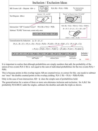
Another way to visualize the communication channel is in terms of an overlay of a Signal Plane divided
(equally) into “0”s and “1”s and a Detection Plane which characterizes how the “0”s and “1”s are detected
and is structured as shown so that when we overlay the two planes we obtain an Outcome Plane with four
distinct regions whose areas represent probabilities of the four product (joint) states { 0R0, 0R1, 1R0, 1R1}
(similar to the tree outputs).
In this representation the total probability of a “0” P(0) can be thought of as decomposed into two parts
summed vertically over the “0”-half of the bottom plane shown by the break arrow P(0) = P(0,R0) + P(0,R1)
[Note: summing on the “1”-half of the bottom plane yields P(1) = P(1,R0) + P(1,R1).]
Similarly the total probability P(R0) can be thought of as decomposed into two parts summed horizontally
over the “R0”-portion of the bottom plane shown by the break arrow P(R0) = P(R0,0) + P(R0,1); similarly
we have P(R1) = P(R1,0) + P(R1,1).
The Total Probability of a given state is obtained by performing such sums over all joint states.
88

20. Log-Odds Ratio - Add & Subtract Measurement Information
Note:
Revisit Binary Comm Channel P( R0 | 0) = .95 P ( R1 | 1) = .90 P(0)=.5
E = “1”
P( R1 | 0) = .05 P ( R0 | 1) = .10 P(1)=.5
Ec = “0”
Relation between  P (1 | R1 )  P (1 | R1 ) e L1
L1 ≡ ln 1 − P(1 | R )  ⇒ e = 1 − P(1 | R ) ⇒

L1
P(1 | R1 ) =
L1 and P(1|R1)  1  1 1 + e L1
 P(1 | R1 )   P (1)   P ( R1 | 1)   P(1)   P( R1 | 1) 
L1 ≡ ln 1 − P(1 | R )  = ln 1 − P(1)  + ln 1 − P( R | 1)  = ln P(0)  + ln P ( R | 0) 
        
 1     1     1 
≡ L0 ≡ ∆L1
 P( R1 | 1) 
Additive Meas Updates for L Lnew = Lold + ∆LR1  P (1) 
 P(0)  ; ∆LR1 = ln P( R | 0) 
Lold = ln   
   1 
Updates
Meas#1: R1 Meas#2: R0 Alternate Meas#2: R1
 .5   P( R0 | 1)   .10   P( R1 |1) 
Lold = ln  = 0 ∆LR0 = ln  .90 
 .5   P( R | 0)  = ln .95 
  
∆LR1 = ln   = ln  
 0   P( R1 | 0)   .05 
 .9  = −2.25129
∆LR1 = ln  = +2.8903
 .05  Lnew = Lold + ∆LR0 Lnew = Lold + ∆LR1
= 2.8903
= 2.8903 + (−2.25129) = .63901 = 2.8903 + 2.8903 = 5.7806
Lnew = 0 + 2.8903
e 2.8903 e.63901 e 5.7806
P(1 | R1 ) = = .947 P(1 | R1 R0 ) = = .655 P (1 | R1 R0 ) = = .997
1 + e 2.8903 1 + e.63901 1 + e 5.7806
96 INDEX
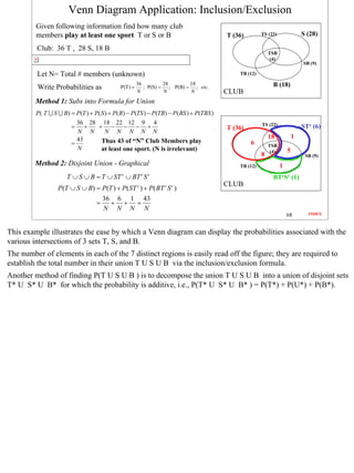
Revisiting the binary communication channel we now compute updates using the log odds ratio which are
additive updates. The update equation simply starts from the initial log odds ratio which is
Lold=ln[P(1)/P(1c)] =ln(.5/.5)=0 for the communication channel. There are two measurement types R1 and
R0 and each adds an increment ∆L determined by its measurement statistics, viz.,
R1: ∆LR1 =ln[(P(R1|1)/P(R1|1c)]=ln(.90/.05) = +2.8903 (positive “confirming”)
R0: ∆LR0 = ln[(P(R0|1)/P(R0|1c)]=ln(.10/.95)= -2.25129. (negative “refuting”)
The table illustrates how easy it is to accumulate the results of two measurements R1 followed by R0 by just
adding the two ∆Ls to obtain
Lnew= 0+2.8903-2.25129=.63901,
or alternately R1 followed by R1 to obtain
Lnew=0+2.8903+2.8903=5.7806.
These log odds ratios are converted to actual probabilities by computing P= eLnew / (1+ eLnew ) yielding .655
and .997 for the above two cases.
If we want to find the number of R1 measurements needed to give .99999 probability of “1” we need only
convert .99999 to an L =ln[(.99999)/(1-.99999)] =11.51 and divide the result by 2.8903 to find 3.98 so that
4 R1 measurements are sufficient.
96

21. Discrete Random Variables (RV) –Key Concepts
• Discrete RVs: A series of measurements of random events
• Characteristics: “Moments:” Mean and Std Deviation
• Prob Mass Fcn: (PMF), Joint, Marginal, Conditional PMFs
• Cumulative Distr Fcn: (CDF) i) Btwn 0 and 1, ii) Non-decreasing
• Independence of two RVs
• Transformations - Derived RVs
• Expected Values (for given PMF)
• Relationships Btwn two RVs: Correlations
• Common PMFs Table
• Applications of Common PMFs
• Sums & Convolution: Polynomial Multiplication
• Generating Function: Concept & Examples
122 INDEX
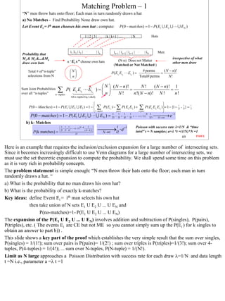
This slide gives a glossary of some of the key concepts involving random variables (RVs) which we shall
discuss in detail in this section. Physical phenomena are always subject to some random components so
that RVs must appear in any realistic model and hence their statistical properties provide a framework for
analysis of multiple experiments using the same model. These concepts provide the rich environment that
allows analysis of complex random systems with several RVs by defining the distributions associated with
their sums and transformations of these distributions inherent in the mathematical equations that are used to
model the system.
At any instant, a RV takes on a single random value and represents one sample from the underlying RV
distribution defined by its probability mass function (PMF). Often we need to know the probability for some
range of values of a RV and this is found by summing the individual probability values of the PMF; thus a
cumulative distribution function (CDF) is defined to handle such sums. The CDF formally characterizes the
discrete RV in terms of a quasi-continuous function that ranges between [0,1] and which has a unique
inverse.
Distributions can also be characterized by single numbers rather than PMFs or CDFs and this leads to
concepts of mean values, standard deviations, correlations between pairs of RVs and expected values.
There are a number of fundamental PMFs used to describe physical phenomena and these common PMFs
will be compared and illustrated through examples. Finally, the relationship between the sum of two RVs
and the concept of convolution and the generating function for RVs will be discussed.
122

22. Transformation of Sample Space: Sum & Difference - 4-Sided Dice
Fair 4-sided dice thrown twice: RVs: Sum= “S” & Absolute Difference “D”
Uniform PMF pD1D2 (d1,d2) = 1/16 Find New PMF pDS(d,s) = ?
Labels: D/S=3/5
d pS(6)
Collapse on s-
d2 S=d1+d2 Rotated to D, S “missing”
axis
points
D=|d2-d1| Coordinates 4
3/5 2/6 1/7 0/8
4 3
2/16 Collapse on
d-axis pD(3)
2/4 1/5 0/6 1/7 2/16 2/16
d2
2
3 D 2/16 2/16 2/16
Collapse on
1
4
1/3 d-axis pD(1)
0/4 1/5 2/6
2 Fold over
s
1/16 1/16 1/16 1/16
3
0
3/
5
0/2 1/3 2/4 3/5 D/S=3/5
S-Axis
2
2/
0 1 2 3 4 5 6 7 8
2/
1
6
4
1
1/
1/
d1
7
1/
5
3
0/
d
0/
8
6
0/
1 2 3 4
0/
S
2
4
pSD ( s, d ) 4
1/
7
1/
1/
5
3
1
pD1D2(d1,d2) d
2/
2/
3
6
4
2
2
3/
2
4
5
3
1
3
D
/S
1/16
=3
0
/5
2
4
d1
2/16
2/16 2/16
1 Absolute Difference Doubles 1/ 2/ 2/ 2/
6 1 1/16
0 6 1 6 1 6 1
Values above S-Axis 1 2/16
2/16
2 1/
6 1
2/
6 1
2/
6 1
3 1/16
1 4 2/ 2/16
2 5 1/
6 1 6 1
3 6 1/16
4
7 1/
6 1
8 1/16
d
1
s 125 INDEX
In the game with 4-sided dice, we are interested in the distribution of the sum random variable S = D1 + D2 ,
pS(s) and not the joint distribution pD1,D2(d1d2). This slide and several to follow illustrate the procedure for
obtaining the desired “marginal” (or collapsed ) distribution pS(s). In the process, we shall develop the
relationship between distributions under transformation of coordinates, and define conditional, and
marginal, distributions involving a pair of RVs {D1,D2}.
We start with the 2- and 3-dimensional dice representations of equally likely outcomes of 1/16 as shown on
the left. Recall that the points (d1, d2) for dice outcomes may alternately be expressed by points (s,d) their
sum and difference coordinates, where s = d1+ d2 and d = d2 - d1 . These coordinate axes are shown in the
top left figure where the sum and difference each take on 7 values: s={2,3,4,5,6,7,8} and d={-3,-2,-
1,0,1,2,3}
We consider a slightly different transformation s = d1+ d2 and |d| = |d2 - d1| and now the absolute difference
|d| takes on only 4 values {0,1,2,3}; this has the effect of doubling the probability values of {1,2,3} by
folding over the negative difference values onto and doubling them. If we label each point in this figure by
the “|d |/ s” values we see for example that the points (d1d2) =(1,4) and (d1d2) =(4,1) at opposite corners of
the grid are both now labeled with |d| / s = 3 / 5 . Labeling all points in this manner and rotating the figure
clockwise 90o so D is up and S is to the right (central figure) we have found the new joint distribution
pSD(s,|d|) as illustrated in the two right figures where points are now labeled by (s,|d|) values. Note that the
new distribution has doubled the positive d values to 2/16 each and that certain coordinate points
(s,|d|)=(3,0) are not occupied (green). The marginal distribution pS(s) defined as the sum of the joint
distribution pSD(s,|d|) over all |d| values and is easily picked off the upper right figure by collapsing values
down along the s-axis. Similarly, the distribution pD(|d|) defined as the sum of the joint distribution
pSD(s,|d|) over all s-values. The table shows the results.
125

23. Common PMFs and Properties -1
RV Name PMF Mean Variance
E[ X ] = ∑ x⋅ p
x = 0 ,1
X ( x) var( X ) = E[ X 2 ] − E[ X ]2
 p X = 1 (success)
Bernoulli p X ( x) = 
1 − p = q X = 0 (failure) E [ X 2 ] = 0 2 ⋅ (1 − p ) + 12 ⋅ p
1-Trial
E [ X ] = 0 ⋅ (1 − p ) + 1 ⋅ p = p
X=x succ.
= p var( X ) = p − p 2 = p (1 − p )
“0” or “1” x “Atomic” RV
successes = pq
0 1
p X (x)
Binomial  n
p X ( x) =   p x q n − x
 
 x
n
n
n - Trials E[ X ] = ∑ x  p x q n − x
6/16
5/16
  var( X ) = npq
x = 0,1, n x=0  x 
X=x Succ. 4/16
3/16
= np
How many Independent 2/1
6
1/16
succ “x” in Bernoulli Trials 0 x
“n” trials ? 0 12 3 4
p X (x)
Geometric p X ( x) =  pq
x −1
x = 1,2, ∞
d ∞ x
 1/2
E[ X ] = ∑ x ⋅ pq x −1 = p ∑q var( X ) =
q
X=x Trials  0 (otherwise) 7/16 dq x =1
6/16
x =1 p2
1- Success 5/16 d  1  +p 1
=p  = =
dq  1 − q  (1 − q) 2 p
4/16
How many One Sequence 3/16  
trials “x” 2/16
1/16 As p decr. Expected num. trials
for “1” succ 0 x “x” for 1-succ must incr.
0 1 2 3 4 5 ... ∞
 x − 1 r x − r
Negative  x − 1 r −1 x − r E[ X ] = ∑ x ⋅ 
 r − 1 p q
 q
 r − 1 p q ⋅ p
p X ( x) =     var( X ) = r ⋅
Binomial  
x=r
p2
succ. on
Geom RV = Neg Binom r
next trial =
X=x Trials ( r −1) succ. in ( x −1) trials
for r=1 succ. p
x = r , (r + 1), ( r + 2), ∞ As p decr. Expected num. trials
r- Successes
Many Sequences “x” for r-succ must incr.
137 INDEX
This table and one to follow compare some common probability distributions and explore their
fundamental properties and how they relate to one another. A brief description is given under the “RV
Name” column followed by the PMF formula and figure in col#2; formulas for the mean and variance are
shown in the last two columns.
The Bernoulli RV X answers the question “what is the result of a single Bernoulli trial?” It takes on
only two values, namely “1”=Success with probability p and “0”=Fail with probability q=1-p.
The Binomial RV “X” answers the question “how many successes X in n Bernoulli trials?” It takes on
values corresponding to the number of successes “X” in “n” independent Bernoulli trials; the sum RV
X=X1+ X2+ ...+Xn of n Bernoulli RVs has nCx tree paths for X=x successes yielding a pmf nCx px qn-x as
shown.
The Geometric RV X answers the question “how many Bernoulli trials X for 1 success?” It takes on
values from 1 to infinity and is the sum of n-1 failed Bernoulli trials followed by one successful trial; the
sum RV X=X1+ X2+ ...+Xn of n Bernoulli RVs has only one tree path with X= x trials yielding 1-success
and so has a pmf qx-1 p1 as shown.
The Negative Binomial RV X answers the question “how many Bernoulli trials X for r- successes?” It
takes on values from r to infinity and is the sum of n Geometric random variables; the sum RV X=G1+
G2+ ...+Gr of “r” Geometric RVs with probability pr-1 qx-r p1 and has x-1Cr-1 tree paths for X=x-1 trials
yielding (r-1)-successes followed by one final success and so has a pmf x-1Cr-1 pr-1 qx-r p1 with x = r, r+1,
... inf, as shown
137

24. Bernoulli/Binomial Tree Structures
RV Name PMF
 p X = 1 (success)
Bernoulli p X ( x) =  (q+p) x Prob
1-Trial 1 − p = q X = 0 (failure)
F
q 0 q
X=x succ. START
p
1 p
“0” or “1” x “Atomic” RV S
successes 0 1
Prob
Binomial  2 p X (x) x
p X ( x) =   p x q 2 − x
2 - Trials  x (q+p)2 F {FF} 0 q2 2C
1/2 q 0
x = 0,1, 2
X=x Succ. q
F
S {FS} 1 qp
p 2C
1/4
How many Independent START
q F {SF} 1 pq
1
succ “x” in Bernoulli Trials x
p S
{SS} 2 p2 2C
“2” trials ? p
S
2
0 1 2
(q+p)2 = q2 + 2pq + p2
= 2C0 p0 q2 + 2C1 p1 q1 + 2C2 p2 q0
138 INDEX
The RVs of the last slide are grouped in pairs {Bernoulli,Binomial} and {Geometric, Negative Binomial}
for a reason. The sum of many independent Bernoulli trials generates a Binomial distribution and similarly
the a sum of many independent Geometric trials generates the Negative Binomial distribution. This slide
and the next give a graphical construction of these trees for these two groups of paired distributions by
repeatedly applying the basic tree structure of the underlying Bernoulli or Geometric tree structure as
appropriate.
In the first panel we show the PMF properties for Bernoulli on the left and on the right we display
Bernoulli tree structure where the upper branch q=Pr{Fail] goes to the state X= 0 and the lower branch p =
Pr[Success] goes to the state X= 1.
In the second panel we show the PMF properties for a simple n=2 trial Binomial. The corresponding tree
structure for this Binomial is obtained by appending a second Bernoulli tree to each output node of the first
trial, thus yielding the 4 output states {{FF}, {FS}, {SF}, {SS}}. We see that there is 2C0 tree paths leading
to {FF} p0q2 , 2C1 tree paths leading to{FS} p1q1 , and 2C2 tree paths leading to {SS} p2q0 , which is
precisely as expected from the Binomial PMF for n=2.
This can be continued for n=3, 4, ... by repeatedly appending a Bernoulli tree to each new node. Further we
see that this structure for n=2 is represented algebraically by (q+p)2 inasmuch as the direct expansion gives
1=q2 + 2q1p1 +p2 ; expanding an expression corresponding to n Bernoulli trials (q+p)n obviously yields the
appropriate Binomial expansion for general exponent n.
Thus the Binomial is represented by the repetitive tree structure or by the repeated multiplication of the
algebraic structure 1=(q+p) by itself n-times to obtain 1n=(q+p)n .
138

25. Geometric/NegBinomial Tree Structures
RV Name PMF
p X (x)
Geometric
 pq x −1 x = 1,2, 1/2
[(1-q)-1 p]
X=x Trials p X ( x) =  7/16
q
F
 0 (otherwise) 6/16
p
1- Success 5/16 F S
4/16 q
How many 3/16 START p
trials “x” for One Infinite 2/16 S
“1” succ Sequence 1/16
p
0 x
0 1 2 3 4 5 ... S
Negative  x − 1 2−1 x − 2 F
Binomial p X ( x) =  p q ⋅ p [(1-q)-1 p ]2 q
 2 − 1 succ. on q F
X=x Trials (2 −1)succ. in ( x −1) trials
next trial S p
S
2- Successes
x = 2,3, 4, ∞ q
F p
p
F S
S
p X (x) START
q
p q
F
1/4 S q F
p S p
3/16 S
S p
Many Infinite
1/8
Sequences S
1/16 F
q
0 x S
q F
0 1 2 3 4 5 ... p
S
p2 (1-q)-2 = p {1+(-2)1-3(-q)1 +[(-2)(-3)/2] 1-4(-q)2 +[(-2)(-3)(-4)/(2)(3)] 1-5(-q)3 + ...} p p
...} S
={ 1C p
1 + 2C
1 pq1 + 3C
1 p1 q2 + 4C1 p1 q3 + p
139 INDEX
This slide first gives a graphical construction of a Geometric tree from an infinite number of Bernoulli
trials and then shows how the Negative Binomial tree is the result of appending a Geometric tree to
itself in a manner similar to that of the last slide. In the first panel we repeat the PMF properties for
Geometric RV. On the right side of this panel we display Geometric tree structure whose branches end
in a single success. This tree has a Bernoulli trial appended to each failure node and is constructed from
an infinite number of Bernoulli trials. The 1st Bernoulli trial yields X=1 with p=Pr[Success] and this
ends the lower branch; its upper branch yields X=0 with q=Pr{Fail]; this failure node spawns a 2nd
Bernoulli trial which again leads to X=1 or X=0; this process continues indefinitely. It accurately
describes the probabilities for a single success in 1, 2, 3,... inf number of trials and is algebraically
represented by the expression 1=[(1-q)-1 p] which expands to [1 + q1 + q2 + q3 +....]*p corresponding to
exactly 0, 1, 2, 3,... “failures before a single success”
In the second panel we show the PMF properties for an r=2 Negative Binomial; on the right we display
the Negative Binomial tree structure obtained by applying the basic Geometric tree to each node
(infinite number) corresponding to a 1st success. This leads to a doubly infinite tree structure for the r=2
Negative Binomial which gives the number of trials X =x required for r=2 successes. We can verify the
first few terms in the Negative binomial expansion given under PMF in the lower panel using the tree.
This process may be extended to r=3, 4, ... successes by repeatedly applying the Geometric tree to each
success node. For n=2, direct expansion of the algebraic identity 12=[(1-q)-1 p]2 yields { 1C1 p + 2C1 pq1
+ 3C1 p1 q2 + 4C1 p1 q3 + ...}p in agreement with the n=2 Negative Binomial terms in the table. In an
analogous fashion expansion of 1r=[(1-q)-1 p]r yields results for the r-success Negative Binomial. Note
that the “Negative” modifier to Binomial is a natural designation in view of the (1-q)-1 term in the
algebraic structure.
139

26. Bernoulli, Geometric, Binomial & Negative Binomial PMFs
• Bernoulli RV as Probability “Indicator” for Outcomes of a Series of
Experiments representing a two different Event types, namely,
E1: “Success in 1 trial” X = Bernoulli RV Binomial b(k;n,p)
n = # trials , k = # successes
E2: “ N1 is #Trials for 1stsuccess“ N1 = Geometric RV K=# Succ
for n- trials
n  n
K = ∑ Xi p K (k ) =   p k q n − k
k
i =1  
n
K = ∑ Xi
Bernoulli Bernoulli Process Sum n Indep. i =1
Single RV , Two Outcomes 1 Bernoulli trial for Bernoulli RVs “X” E ( K ) = µ K = np
Event E1 var( K ) = σ K = npq
2
 p X = 1 (success)
p X ( x) =  p X ( x) = p
1 − p = q X = 0 (failure)
Neg. Binomial bn(nr;r,p)
Sum r Indep.
1 = # trials , 0,1 = # successes Geometric RVs
Geometric Process nr = #trials for r successes
”N1”
E ( X ) = µ X = p ; var( X ) = σ X = 0
2
n1 Bernoulli trials for  n − 1
pNr (nr ) =  r  p r q nr − r
Event E2  r −1 
r
pN1 (n1 ) = p1q n1 −1 N r = ∑ ( N1 )i r
i =1 N r = ∑ ( N1 )i
i =1
1
E[ N r ] = µ N r = rE[ N1 ] = r
Nr =# Trials p
for r-Succ. q
var( N r ) = σ N r 2 = r var( N1 ) = r
p2
140
The Bernoulli RV “X” is the basic building block for other RVs ( “atomic” RV ) and has a PMF
distribution with only two outcomes X=1 with probability p and X=0 with probability q=1-p . We have seen
that n such Bernoulli variables when added yield a Binomial PMF {b(x;n,p), x=0,1,2,...,n} which gives the
“#successes “x” for “n” trials.
We have also seen that this Binomial PMF can be understood by repeatedly appending the Bernoulli tree
graph to each of its nodes (repeated independent trials) thereby constructing a tree with 2n outcomes
corresponding to the n Bernoulli trials, each with two possible outcomes.
Alternately, the Geometric PMF can be constructed by repeatedly appending a Bernoulli tree graph, but this
time only to the failure node, an infinite number of times, thereby constructing a tree with an infinite
number of outcomes all of which correspond to “x-1” failures and exactly 1 success for x=1,2, ...., inf.
Just as the Bernoulli tree graph is a building block for the Binomial tree graph, the infinite Geometric PMF
tree graph is a building block for the Negative Binomial. The Negative Binomial tree graph for r=2
successes is constructed by appending a Geometric tree graph to itself, but this time only to the success
nodes, resulting in a doubly infinite tree graph corresponding to exactly “x-1” failures and exactly 2
successes for x= 2,3 ...., inf. Repeating this process r-times yields the r-fold infinite tree graph
corresponding to exactly “x-1” failures and exactly r successes for x= r,r+1, ...., inf.
The mathematical transformations relating Bernoulli, Binomial,Geometric and Negative Binomial are
shown in this slide.
140

27. Common PMFs and Properties-2
RV Name PMF Mean Variance
E[ X ] = ∑ x⋅ p
x = 0 ,1
X ( x) var( X ) = E[ X 2 ] − E[ X ]2
 "m-marked" "(N-m) = unmarked"
x from (n-x) from
Hyper-  m ( N − n) m ( N − m)
 m  N − m E[ X ] = n ⋅ = n ⋅ p var( X ) = n ⋅ ( N − 1) ⋅ N ⋅ N
geometric   x   N
    n−x  ; x ≤ x ≤ x
X=x -succ pX ( x) =  where p = m / N is the
 N
min max
( N − n)
N= fixed pop    "initial" probability of var( X ) = ⋅n⋅ p⋅q
  n ( N − 1)
m= tagged  0 ; Otherwise drawing a marked item

n=test sampl m ∈ [1, N ] ; n ∈ [1, N ] ; ( N − m − n) ≤ x ≤ min(m, n)
w/o rplcemt PMF Derives from  N   m + ( N − m)   m   N − m   m   N − m   m N − m  m  N − m 
Binomial Identity  =  =    +   + +   + +   
n  n   0   n   1   n −1   x  n − x   n  0 
n≤m≤ N
Poisson  ( a x / x !)
 x = 0,1, 2, ∞
Trials p X ( x) =  ea
E[ X ] = a var( X ) = a
0 Otherwise
X=x Succ 
Limit of Binomial
a = lim(n ⋅ p) = λ ⋅ t = (aver. arrival rate)*time
n →∞
p →0
Zeta(Zipf) 
 ( )
 1 xs
p X ( x; s ) =  ζ ( s) =
"ζ − term "
x = 1, 2, ; s >1 (
∞
E[ X ; s ] = ζ 1s ) ⋅ ∑ x⋅ 1s
x
(
∞
Var ( X ; s ) = ζ 1s ) ⋅ ∑ x2 ⋅ 1s − E[ X ; s]2
x =1
x
n - Trials ζ (s) x =1
X=x Succ.


 0 Otherwise (
∞
= ζ 1s ) ⋅ ∑ 


1 

 = ζζ( s( −1)
s)
= ζ ζ( s(−)2) −
s ( ζ (s) )
ζ ( s −1) 2
 x s −1 
−1 x =1
 
( )
∞ ∞
ζ (1.5) ζ (2.5) 2
∑
x =1
= 1 ⇒ C =  ∑  1s   = ζ 1s )
C 
 
 
 xs 
 
 
 x =1  x  
(
E[ X ; s = 3.5] = ζζ( s( −1) = 1.191
Var ( X ; s = 3.5) = ζ (3.5) − ζ (3.5)
s)
= .856
Riemann Zeta Fcn ζ (s)
141 INDEX
This second part of the Common PMFs table shows the Hyper-geometric, Poisson and Riemman Zeta (or
Zipf ) PMFs
The Hyper-geometric RV “X” answers the question “how many successes (defectives) X are obtained
with n test samples (trials without replacement) from a production run (sample space) that contains m
defective and N-m working items?” X takes on values corresponding to the number of successes
(defectives) “X” in “n” dependent Bernoulli trials; the distribution is best understood in terms of the
Binomial identity NCn = mC0 N-m Cn + ...+ mCx N-m Cn-x +... + mCm N-m Cn-m which when divided by NCn
yields the distribution mCx N-m Cn-x where X takes on values x=[xmin, xmax] where xmin=N-n-m and xmax=
min(n,m).as allowed by the combinations w/o replacement
The Poisson RV “X” answers the question “how many successes X in n Bernoulli trials with n very
large?” We shall discuss this in more detail in the second part of the course where we pair it with a
continuous distribution. For now it is sufficient to know that it represents a limiting behavior of the
Binomial PMF in the limit that n-> inf and its terms represent single terms in the expansion of ea where a
=λ∗ t is called the Poisson parameter, where λ is a “rate” and t is a time interval for the data run. The PMF
is therefore the ratio of the single term in the expansion to ea over ea which is
pX(x)={ ax/ x!} / ea for x=0,1,2,3,... The Poisson RV has many applications in physics and engineering.
The Riemman Zeta RV “X” has applications to Language processing and prime number theory and its
properties are given in the table. Note that the exponent must satisfy α >0 in order to avoid the harmonic
series which will does not converge and therefore cannot satisfy the sum to unity condition on the PMF.
141

28. Chapter 5 – Continuous RVs
Probability Density Function (PDF)
f X (x)
Event E = {x : a ≤ x ≤ b}
:
b
Pr[ x ∈ E ] = ∫ f X ( x)dx = ∫ f X ( x)dx Pr[a ≤ x ≤ b]
E a a x
2.0 b
Pr[ x = 2.0] = ∫f
x = 2.0
X ( x)dx = 0 Prob at a point = 0 Except for δ-fcn at a point
αδ ( x − x0 ) uniform
Mixed Continuous & Discrete Outcomes – Dirac δ-fcn f X (x) β
(b − a )
β
f X ( x) = αδ ( x − x0 ) +
(b − a )
b x0 + ε
x
∫ αδ ( x − x )dx = ∫ ε αδ ( x − x )dx =α
a
0
x0 −
0
a x0 b
Sampled Continuous Fcn g(x) f X (x) α k δ ( x − xk )
n
g (x)
f X ( x ) = ∑ α k δ ( x − xk )
k =0
b
α k = ∫ g ( x)δ ( x − xk ) =g ( xk )
a x0 x1 xk xn x
2/24/2012 3
In Discrete Probability a RV is characterized by its probability mass function (PMF) pX(x) which
specifies the amount of probability associated with each point in the discrete sample space. Continuous
probability generalizes this concept to a probability density function (PDF) fX(x) defined over a
continuous sample space. Just as the sum of pX(x) over the whole sample space must be unity, the
integral of fX(x) over the whole sample space must also be unity. An event E is defined by a sum or
integral over a portion of the sample space as shown by the shaded area in the upper figure between x=a
and x=b.
The middle panel gives an example of a mixed distribution containing continuous uniform distribution
β/(b-a) and a Dirac δ-function at the point x0 α∗ δ(x-x0) corresponding to a discrete contribution at that
point. The uniform distribution is shown as a continuous horizontal line at “height” y = β between a and
b and the Dirac δ-function is shown with an arrow corresponding to a probability mass “α” accumulated
at a single point x=x0.. The integral over the continuous part gives (b-a)* β/(b-a) = β and the integral of
the Dirac δ-function α∗ δ(x-x0) over any interval containing x0 yields α. Thus, in order for this
expression to be a valid probability density function, we require the sum of the two contributions be
unity: α+ β =1 .
Consider the continuous curve fX(x) = g(x) in the bottom panel and take the sum of products αk*δ(x-xk).
Is this a valid discrete “PMF”? In order for this to be so the sum of the contributions αk must be unity.
Does it represent a digital sampling of g(x)? No, in order to actually write down an appropriate
“sampled” version of g(x), we need to develop a “sampling” transformation Yk=Yk(X) for k=0,1,2,...,n so
as to transform the original continuous fX(x) to a discrete fY(yk) (See slide#26 )
3

29. Cumulative Distribution Function (CDF)
x
FX ( x) = Pr[ X ≤ x] = ∫ f X ( x ') dx ' Probability Density PDF
x '=−∞
integrates to yield CDF
fX(x) fX(x) PDF
Bdy Values : FX (−∞) = 0 ; FX (+∞) = 1 PDF
1 1
¼ δ(x-1)
1/2
Monotone Non - decr. : FX (b) ≥ FX (a ) ; if b ≥ a 0 x x
0
0 1/2 1 3/2 0 1/2 1 3/2
Prob Interpretation : Pr[a ≤ x ≤ b] = FX (b) − FX (a)
FX(x) CDF FX(x) CDF
Density PDF : d
dx FX ( x) = f X ( x)
1 1
¼
1/2 1/2
or, dFX ( x) = FX ( x + dx) − FX ( x) = f X ( x)dx
0 x 0 x
0 1/2 1 3/2 0 1/2 1 3/2
2/24/2012 7
The cumulative distribution function (CDF) for a continuous probability density function fX(x) is defined
in a manner similar to that for discrete distributions pX(x) except that the cumulative sum over a discrete
set is replaced by an integral over all X less than or equal to a value x. This integral yields a function of
“x” FX(x) = Pr[X<=x] which has the following important properties
(i)FX(x) always starts at 0 and ends at 1
(ii)FX(x) is continuous,
(iii)FX(x) is non-decreasing,
(iv)FX(x) is invertible; i.e., FX -1 (x) exists, and
(v)The density fX(x)=d/dx{FX(x)} (since exact differential d FX(x) = FX(x+dx) - FX(x) = fX(x)dx )
It is important to note all five properties of FX(x) as they have important consequences.
The figure shows the relationship between the density fX(x) and the cumulative distribution FX(x) for two
cases (i) two regions of constant density (two “boxes”) and (ii) one region of constant density plus a delta
function (one “box” and an arrow “spike”) .
In case (i) FX(x) ramps from a value of 0 to ½ in the region [0, ½ ] from the 1st constant density box, then
remains constant at ½ over the region [ ½ , 1] and finally ramps from ½ to 1 from the 2nd constant
density box. Note that the slopes of the two ramps are both “1” in this case and that the total area under
the density curves 1* [1/2-0] + 1* [3/2-1] = 1.
In case (ii) FX(x) ramps from a value of 0 to ½ in the region [0, 1] by virtue of the constant “½” density
box, then jumps by “1/4” because of the delta function, and finally continues its ramp from the value ¾ to
1. Note that this is simply the superposition of a constant density of “ ½“ plus a delta function ¼∗ δ(x-
1), and again the total area under the density curves ½ * [3/2-0] + ¼ = 1
7

30. Transformations of Continuous RVs
• Transformation of Densities PDFs in 1 dimension
• Transformation of Joint Densities PDFs in 2 or more dimensions
• Two Methods:
1) CDF Method:
Step#1) First find CDF FX(x) by integrating fX(x)
Step#2) Invert y=g(x) transformation y = g(x) ⇒ x = g −1 ( y )
& use it to write FY ( y ) = Pr[Y ≤ y ] in terms of the known FX(x)
(Note y= g(x) may not be “one-to-one” “multiplicity”)
y '= y
Step#3) Differentiate wrt y: d d
fY ( y ) =
dy
FY ( y ) =
dy ∫f
y '= −∞
Y ( y ' )dy '
2) Jacobian Method: Transform PDF fY(y) using derivatives f X ( x)
fY ( y ) =
Express everything in terms of variable y dy dx
fY ( y )dy = f X ( x)dx ; y = g ( x) f X ( x = g −1 ( y ))
=
g ' ( x = g −1 ( y ))
Note absolute value
2/24/2012 14
It is very important to understand how probability densities change under a transformation of coordinates
y=g(x). We have seen several examples of such coordinate transformations for discrete variables,
namely,
(i) Dice: Transform from individual dice coordinates (d1, d2) to the sum and difference coordinates (s, d)
corresponding to a 90 degree rotation of coordinates, and
(ii) Dice: Transform from individual dice coordinates (d1, d2) to the minimum and maximum coordinates
(z, w) corresponding to corner shaped surfaces of constant minimum or maximum values.
There are two methods for transforming the densities of RVs, namely (i) the CDF-method and (ii) the
Jacobian Method. While they are both quite useful for 1-dimensional PDFs fX(x), the Jacobian method is
best for transforming joint RVs .
The CDF method involves three distinct steps as indicated on the slide, namely (i) compute CDF FX(x),
(ii) Relate FY(y) = Pr[Y<=y] to FX(x) and then invert the transformation x = g-1(y) and substitute to find
FY(y) with a redefined y domain, and (iii) differentiate wrt “y” to obtain the transformed probability
density for the RV Y: fY(y). Note that if the function is multi-valued and therefore not invertible, it must
be broken up into intervals for which it is invertible and appropriate “fold-over” multiplicities must be
accounted for.
The Jacobian Method uses derivatives of the transformation to transfer densities from the original set of
RVs to the new one; the Jacobian accounts for linear, areal, and volume changes between the coordinates.
In one dimension the Jacobian is simply a derivative and is obtained by transferring the probability in the
interval x to x+dx: fX(x)dx to the probability in the interval y to y+dy: fY(y)dy Equating the two
expressions yields fY(y) =fX(x) / |dy/dx| = fX(g-1(y) ) / |dy/dx|. Note that the absolute value is necessary
since fY(y) must always be greater than or equal to zero.
14

31. Method#1
Transformation of Continuous RV - CDF Method
Resistance X = R Step#1 Compute FX(x) CDF= FX(x)
PDF = fX(x)
1/ 200 900 ≤ r ≤ 1100
f R (r ) =  1
 0 Otherwise
1/200
r '=r  0 r < 900

FR (r ) = Pr[ R ≤ r ] = ∫ f R (r ')dr ' = (r − 900) / 200 900 ≤ r ≤ 1100
0
r '=−∞  1 r > 1100 900 1100 x

Conductance Y = 1/R Step#2 Transform to FY(y)
PDF = fY(y)
FY ( y) = Pr[Y ≤ y] = Pr[ R ≥ 1/ y] = 1 − Pr[ R ≤ 1/ y]
6050
 1− 0 = 1 1/ y < 900 CDF= FY(y)
 1
 ( − 900)
 y 1
= 1 − FR (1/ y) = 1 − 900 ≤ 1/ y ≤ 1100
 200
 1 −1 = 0 1/ y > 1100 4050


Step#3 Differentiate FY(y)  0 y<
1
 1100
 1 0
d  1 1
fY ( y ) = FY ( y ) =  ≤ y≤ 1/1100 1/900 y
dy  200 y 2 1100 900
 0 1
y>

 900
2/24/2012 15
The Resistance X=R of a circuit has a uniform probability density function fR(r)=1/200 between 900 and
1100 ohms as shown in the top panel; the corresponding CDF FR(r) is the ramp function starting at “0”
for R<=900 and reaching “1” at R=1100 and beyond as shown. The detailed analytic function is given in
the slide and represents the result of Step#1 in the CDF-Method.
The problem is to find the PDF for the conductance Y=1/X = 1/R. We first down the definition for FY(y)
for a given value Y=y and then re-express it as a function of R =1/Y
FY(y) =Pr[Y<=y] = Pr[R>=(1/y)] = 1-Pr[R<=(1/y)]
= 1 – FR(1/y )
This last expression is now evaluated in the lower panel of the slide by substituting r=1/y into the
expression for FR(1/y ) of the upper panel. Note the resulting expression has been written down by direct
substitution and the intervals have been left in terms of 1/y. (This constitutes step#2 of the method).
Finally, differentiating FY(y) wrt “y” we find (step#3) the desired PDF fY(y); we have also “flipped” the
“1/y” interval specifications and reordered the resulting “y” intervals in the customary increasing order.
As seen in this example, the CDF method requires careful attention to the definition of the FY(y) defined
in terms of cumulative probability of the variable Y. Since Y=1/R, this leads to FY(y) = 1-
FR(1/y ) and a reverse ordering of the inequalities for the intervals.
15

32. Transformation of Continuous RV - Derivative (Jacobian) Method
Method#2
PDF
1 / 200 900 ≤ r ≤ 1100 6050
f R (r ) = 
 0 Otherwise 1
fY ( y ) =
fY ( y )dy = f R (r )dr ⇒ Find fY ( y ) 200 y 2
dr f (r ) 4050
fY ( y ) = f R (r ) = R
dy | dy / dr | 1 1
f X ( x) =
200 dy y=
fY ( y ) =
f R (r )
=
(1 / 200)
900 dx R
| −1 / r |2
y2 hyperbola: xy = 1
dy
slope =
dx
1 1 1
fY ( y ) = for ≤ y≤
200 y 2 1100 900 1100
x=R
Note: fY(y) is large for small slope & vice versa.
Same Differential Area (Probability) is mapped via hyperpola
to yield the tall high and short fat strip areas shown for fY(y)
2/24/2012 16
The Jacobian Method is much more straight forward and moreover has a very intuitive visualization in
the 3-dimensional plot shown on this slide. The uniform probability density function fR(r)=1/200 between
900 and 1100 ohms is written explicitly in the first boxed equation. The Jacobian method just takes the
constant fR(r) = 1/200 and divides it by the magnitude of the derivative |dy/dr|=|-1/r2| = y2 to yield directly
fY(y)=1/(200y2) for y ε [1/1100, 1/900].
The 3-dimensional plot shows exactly what is going on:
i) The original uniform distribution fX(x)=1/200 displayed as a vertical rectangle in the x-z plane ii)
Sample strips at either end with width “dx” have the same small probability dP= fX(x)dx as shown At
R=900, the density fX(x) is divided by the large slope |dy/dx| yielding a smaller magnitude for fY(y) as
illustrated, but this is compensated by a proportionately larger “dy”and thus transfers the same small
probability dP= fY(y)dy.
iii) Conversely, the strip at R=1100 is divided by a small slope |dy/dx| and yields a larger magnitude for
fY(y), which is compensated by a proportionately smaller “dy” again transferring the same dP.
iv) The end point values of the transformed density fY(y) are illustrated in the figure. The strip width “dx”
cuts the x-y transformation curve at two red points which have a “dy” width that is small at x =1100 and
large at x = 900 as determined by the slope of the curve. The shape in between these end points is a
result of the smoothly varying slope of the transformation hyperbola shown in the x-y plane.
Thus the slope of the transformation curve (hyperbola xy=constant in this case) in the x-y plane
determines how each “dx” strip of the uniform distribution fX(x)=1/200 in the x-z plane transfers to the
new density fY(y) shown in the z-y plane. This 3-dimensional representation de-mystifies the nature of
the transformation of probability densities and makes it quite natural and intuitive for 1-dimensional
density functions. It is easily extended to two-dimensional joint distributions.
16

33. Transformation of Continuous RV – Example 3 “Multiplicity Factor”
Gaussian PDF : y
x2
1 −
f X ( x) = e − ∞ < x < +∞
2
2π Not a 1-1 mapping
Double
Density Pts
Find PDF for Y = X 2 ( −∞, ∞) → (0, ∞) Fold-over
1 −
y
density is doubled x
e 2
f X (x) 2π
f Y (y) = 2 =2
dy/dx 2 y 1 −
y
y 2π y
e 2
1 −
= e 2 for 0 < y < +∞ x2
2πy 1 −
2π
e 2
Two Equal
GeneralRule : Contributions
from –x & +x
f X (x)
fY (y) = α ⋅
dy/dx y
Double
α = multiplici factor
ty Density Pts
" fold - over" y = x2
x
2/24/2012 18
The transformation of a Gaussian PDF under the transformation Y=X2 is easily computed using the
Jacobian method provided one incorporates a multiplicity factor α as shown in the boxed density
equation . The multiplicity factor arises because there are two contributions to the same y-value one
from –x and the other from +x as illustrated in the upper figure; thus folding the parabola across the x=0
symmetry line yields twice the density on positive x and this corresponds to a multiplicity factor α=2 in
the boxed density transformation equation.
The 3d plot shows the original Gaussian density function (grey) in the x-z plane, the transformation y=x2
in the x-y plane, and the resulting distribution shown as a dashed curve in the y-z plane. The two thin
vertical slices at –x and +x are mapped to the same y-value and hence doubles the density contribution to
fY(y) as shown.
18

34. Analog to Digital (A/D) Converter - Series of Step Functions
Continuous Representation of Discrete “sampled” Distributions Y (OUT)
3
A/D converter
Mapping Fcn Y = g( X ) = k +1 ; k < x ≤ k +1 -3
2
1
-2 -1
X
Mapped Density fY (y) = ∑ αk ⋅ δ(y − yk ) 0
-1 1 2 3 (IN)
k -2
a) Exponential b) Gaussian b) Uniform
1 −x2 / 2
ae − ax PDFX = f X ( x) = e 1 0 ≤ x ≤ 10
x≥0 2π PDFX = f X ( x) = 
PDFX = f X ( x) =  0 otherwise
 0 x<0 −∞ < x < ∞
 k k
α k = ∫ f X ( x)dx =  x =∫ −1
k
 ae − ax dx = −e − ax x≥0 k
1 − x2 / 2 k
k − (k − 1)
k
x = k −1 αk = ∫ 2π
e dx = ϕ (k ) −ϕ (k − 1) αk = ∫
1
dx =
x = k −1  0 x<0
x = k −1 10 10
 x=k
1 − x2 / 2
x = k −1
1
e − ak (ea − 1) x ≥ 0
ϕ (k ) ≡ ∫ 2π
e dx ; k ∈ (−∞, ∞ ) =
10
; k = 1, 2,L ,10
= ; k = 1, 2,... x =−∞
 0 x<0
∞ 10
1
fY ( y ) = ∑ e − ak (e a − 1) ⋅ δ ( y − k ) fY ( y ) = ∑ α k ⋅ δ ( y − yk ) fY ( y ) = ∑ δ ( y − k)
k =1 k k =1 10
e − (0.1) k (e0.1 − 1) = .105 ⋅ e − (0.1) k fY(y)
fY(y)
k αk
fY(y)
0.1 α kδ ( y − k )
1 0.095 1/10
0.095 2 0.086
0.050 3 0.078 y y
0 1 5 10
y
0 10 20 11 0.035
2/24/2012 26
In discussing the half-wave rectifier on the last slide we found that the effect of a “zero” slope
transformation function was to pile up all the probability in the x-interval into a single δ-function at the
constant y=“0” value associated with that part of the transformation. Here we extend that concept to a
“sample & hold” type mapping function typical of an Analog to Digital (A/D) converter. The specific
mapping function y=g(x) = k+1 for k < x ≤ k+1 is illustrated in the grey box as a series of horizontal
steps over the entire range of x [-3, 3]; the y-values for these steps range from y=-2 to y=+3. Each
horizontal (zero-slope) line accumulates the integral of fX(x) from x=k to k+1 onto its associated y-value
shown as a red circle with the point of a δ-function arrow pointing up out of the page and having an
amplitude given by the integral for that interval denoted by the symbol αk.
The table shows several examples of a digitally sampled representation for a) Exponential, b) Gaussian,
and c) Uniform distributions in the three columns. The rows of the table give the specific continuous
densities for each, the computations for the amplitudes of the discrete digital samples αk, the resulting
sum of δ-functions, and finally a plot showing arrows of different lengths to represent the δ-functions of
the sampled distributions.
26

35. Order Statistics - General Case n Random Variables
General Case n Variables: X1,, X2 , ... ,, Xn RVs fX (x) fX(y)dy
Assume RVs are Indep and Identically Distributed (IID) FX ( y ) 1 − FX ( y )
{X1,, X2 , ... ,, Xn } fX(x)
f X 1 X 2 L X n ( x1 x 2 L x n ) = f X ( x1 ) ⋅ f X ( x 2 ) ⋅ L ⋅ f X ( x n )
Reorder {X1,, X2 , ... ,, Xn } as follows: fX(y)dy
Y1,= smallest {X1,, X2 , ... ,, Xn } all Yk <y y y+dy all Yk > y
Y2= next smallest {X1,, X2 , ... ,, Xn } Y1 |Y2 |… |Yj-1 Yj+1 | Yj+2 | … | YN
jth “order
Yj= jth smallest {X1,, X2 , ... ,, Xn } (j-1) RVs
statistic” (n-j) RVs
Yn= largest {X1,, X2 , ... ,, Xn }
Each IID: P[Yj ≤ y]= FX(y) P[Yj > y]= 1 - FX(y)
Y1< Y2 < Yj <… < Yn
[FX(y)]j-1 [1 - FX(y)]n-j
Same PDF in variable “y” fX(y)
Diff’l Prob.
Find PDF for the jth “order statistic” “one sequence” = ( FX ( y ) ) j −1 ⋅ f X ( y )dy ⋅ (1 − FX ( y ) )n − j
Pr[ y ≤ Y j ≤ y + dy ] = fY j ( y )dy ; j = 1, 2,L , n jth order statistic
3! [φ| X1 | X2 X3]
j=1: [φ| Y1 |Y2 Y3 ] 0! 1! 2!
=3 [φ| X2 | X1 X3]
Case n=3 {Min, Mdl, Max};Y2 = “Mdl“statistic. Min [φ| X3 | X1 X2]
Y2 could be any one of {X1,, X2 , X3 } 3!
[X2,| X1 | X3], [X3,| X1 | X2]
j=2: [Y1 |Y2 | Y3 ] =6 [X1,| X2 | X3], [X3,| X2 | X1]
1! 1! 1! [X1,| X3 | X2], [X2,| X3 | X1]
Mdl
There are 3! = 6 orderings; however, we partition into 3 [ X2 X3 |X1 |φ]
3!
groups and permutations within a group is irrelevant; j=3: [Y1 Y2 | Y3 | φ] 2! 1! 0!
=3 [ X1 X3 |X2 |φ]
[ X1 X2 |X3 |φ]
Max 48
2/24/2012
Order Statistics for the general case of n IID Random Variables is detailed on this slide. The n IID RVs
{X1, X2,..., Xn} are re-ordered from the smallest Y1 to the largest Yn and the jth Y in the sequence Yj is
called the “jth order statistic”. Again we fix a value Y=y and consider the continuous range of re-ordered
Y-values illustrated in the figure: the small interval from y to y+dy contains the differential probability
for the jth order statistic Yj given by fX(y)dy; all Y-values less than this belong to the Y1 through Yj-1 and
those greater belong to Yj+1 through Yn as shown in the inset figure. Now for each of the Ys on the left we
have the probability Pr[Y1 ≤ y] = FX(y), Pr[Y2 ≤ y] = FX(y), ... Pr[Yj-1 ≤ y] = FX(y), and because they are
IID the total probability of those on the left is Pr[Yleft ≤ y] = [FX(y) ]j-1; similarly on the right we find
Pr[Yright ≤ y] = [1-FX(y) ]n-j. So for the reordered Ys the differential probability is just the product of these
three terms multiplied by a multiplicity factor α, viz.,
dP = Pr[y≤ Yj ≤ y+dy]= f Yj (y) dy = α [FX(y) ]j-1 fX(y) [1-FX(y) ]n-j dy
The multiplicity factor α results from the number of re-orderings of {X1, X2,..., Xn} for each order
statistic Yj ; arguments for n=3 and n=4 are illustrated on this slide and the next. These arguments look
(in turn) at each order statistic min, middle(s), and max and compute in each case the number of distinct
arrangements of {X1, X2,..., Xn} that yield the three groups relative to the “separation point” Y=y and
arrive at multinomial forms dependent upon the orderings for each statistic. The specific multiplicity
factors for the cases for n=3,4 are easily found to be
α = 3C (j-1),1,(3-j) = 3! / [(j-1)! 1! (3-j)!] ; α = 4C (j-1),1,(4-j) = 4! / [(j-1)! 1! (4-j)!]
and the final results for the PDF of the jth order statistic f Yj (y) in these cases are
fYj (yj) = 3C (j-1),1,(3-j) [FX(yj) ]j-1 fX(yj) [1-FX(yj) ]3-j for j=1,2,3 (n=3)
fYj (yj) = 4C (j-1),1,(4-j) [FX(yj) ]j-1 fX(yj) [1-FX(yj) ]4-j for j=1,2,3,4 (n=4)
48

36. Random Processes – Introduction - Lec#4
• Time Series Data = Physical Measurements in time
• Random Process = Sequence of random variable realizations
– Geiger Counter Sequence of “detections” - Poisson Process
– Communication Binary Bit Stream - Bernoulli Process “ 01001…”
– E&M Propagation Phase (I-Q components) - Gaussian Process
• Arrival Event: Success =“arrival” (of an event in time)
• Interarrival Times for Random Processes
– Not only interested in how many successes K (“ arrivals”) there are
– But also interested in “specific time of arrivals,” e.g., TK = time of kth arrival
– DSP Chip Interrupts:
Random Number of Interarrival
• Time between interrupts Process Arrivals Times
• used for data processing Geiger
Poisson Exponential
– Waiting on Telephone: Counter
• “you are 10th customer in line and … Binary Bit
Stream Bernoulli Geometric
• your wait will be approximately “7 minutes”
2/24/2012 61
Observations of physical processes produce measurements over time which almost always have
components described by a random process. Some examples are Geiger counter detections (Poisson
Process), Binary bit streams (Bernoulli Process) and Electromagnetic wave I, Q Phase components
(Gaussian Process).
Because, these processes take place over time, the notion of a “success” is translated to an “arrival” at a
specific time. Moreover, we are not only interested in how many successes K there are, but also their
specific arrival times, i.e., we would like to know the time of the kth arrival Tk. This has application to
many physical processes such as the timing of DSP chip interrupts relative to their “clock cycles” and the
queuing of customers in a telephone answering system. In both cases you want to make sure the system
can handle the “load” in an appropriate manner; for the DSP chip you need to minimize the number of
times you are near the leading or trailing “edge” of the timing pulse in order to avoid errors, while for the
telephone answering service, the 10th customer, would like to know how long he must wait in the queue
before being served.
61

37. Multi-User Digital Communication “CDMA” Arrival Slots
• Two signals s1 , s2 ;Decode s1 or s2 in given time slot s1 Decoded
P|s1,1]= P[1|s1] P|s1] “success”
• a priori Prob: P[s1]=3/4 ; P[s2]=1/4 P[1|s1] =(2/3)(3/4) =1/2 p1=1/2
S1 2/3
• Decoding Statistics: 1/3
P[s1] 3/4 P[0|s ]
P|s1,0]=1/4
decoded “1” : P[1|s1]=2/3 ; P[1|s2]=2/3 Time
1
s1 Not
Slot #4 P[1|s2] P|s2,1]= P[1|s2] P|s2] Decoded
not decoded “0” : P[0|s1]=1/3 ; P[0|s2]=1/3 1/4 S2 =(2/3)(1/4) =1/6 “failure”
P[s2]
2/3
q1=1/2
1/3
Nr time slots (“trials”)  n − 1 r n − r P[0|s2]
P|s2,0]=1/12
p N r ( n) =  p q
r-Decodes of s1 p1=q1=1/2  r −1 a priori decode
4 −1 1
1 1 1
1) Pr[ 1st decode in 4th slot] Pr[ N1 = k ] = p N1 (k ) = q k −1
p1 ⇒ Pr[ N1 = 4] = p N1 (4) =     =
 2   2  16
2) Pr[ 4th decode in 10th slot | 3 decodes No memory - slots 6 to 10 1 2 3 4 5 6 7 8 9 10
“1” “1” “1”
in 1st 6 time slots ] 1 1
3
1
1 1 2 3 4
Pr[ N1 = 4] = p N1 (4) = q 3 p =     = 3 “1”s
No Memory
 2   2  16
4
3) Pr[ 2nd decode in 4th slot]  n − 1 r n − r  4 − 1 2 4 − 2 1 3
Pr[ N r = n] = p N r (n) = 
  p q ⇒ Pr[ N 2 = 4] = p N 2 (4) = 
  2 − 1 p q = 3 2  = 16

 r − 1    
4) Pr[ 2nd decode in 4th slot | no decodes No memory of failures in slots 3 & 4 1 2 3 4
“0”“0”
2
in 1st 2 time slots] 1 1 1 2
Pr[ N 2 = 2] = p N 2 (2) = p 2 =   =
 2 4 “Renewal”
{ “means” N2>2 }
Pr[ N 2 = 4 , N 2 > 2 ] p N 2 (4) ( 3 / 16 ) 1
Pr[ N 2 = 4 | N 2 > 2 ] = = = =
Pr[ N 2 > 2 ] 1 − p N 2 ( 2 ) 1 − (1 / 4 ) 4
2/24/2012 78
This example illustrates renewal properties and time slot arrivals of the Geometric and Negative Binomial RV distributions.
In a multiuser environment the digital signals from multiple transmitters can occupy the same signal processing time slot so
long as they can be distinguished by their modulation characteristics. Code Division Multiple Access (CDMA) uses a
pseudorandom code that is unique to each user to “decode” the proper signal source.
Consider two signals s1 and s2 being processed in the same time slot with a priori “system usage” given by P[s1] = ¾ and P[s2]
= ¼ ; further let “1” denote successful and “0” denote unsuccessful decodes respectively. Given that each signal has the same
2/3 probability of a successful decode P[1|s1] = P[1|s2] = 2/3, we can use the tree to find the single trial probability of success
for decoding each signal.
For signal s1 we see that the end state {s1, 1} represents a successful decode and has p1=1/2 ; all other states {s1, 0}, {s2 1},
{s2, 0} represent failure to decode signal s1 with probability q1 = 1/4+1/6 + 1/12 = 1/2. Similarly for signal s2 we see that the
end state {s2, 1} represents a successful decode of s2 and has p2 =1/6 ; all other states {s2, 0}, {s1 1}, {s1, 0} represent failure to
decode signal s2 with probability q2 = 1/12+1/2 + 1/4 = 10/12 =5/6.
We consider successive decodes of s1 as independent trials with probability of success p1=1/2 . Thus, the probability of
having r- successful decodings of s1 in Nr signal processing slots “trials” is given by the Negative Binomial PMF
pNr(n) = n-1Cr-1p1rq1n-r with nr = r, r+1, r+2, .... with p1=q1=1/2
1) Pr of 1st decode (r=1) in 4th slot (N1 =4) is pN1(4) = 4-1C1-1p11q14-1 = 1(1/2)4 = 1/16
2) Pr of 4th decode (r=4) in 10th slot (N4 =10) given 3 previous decodes in 1st 6 slots is found by “restarting the process with
slots #7 , 8, 9, 10 so we need only one decode (r =1) in 4 slots, i.e., N1 =4, which is identical to part 1) and yields
Pr[N4 = 10 | N3=6] = pN1(4) = 4-1C1-1p11q14-1 = 1(1/2)4 = 1/16
3) Pr of 2nd decode (r=2) in 4th slot (N2 =4) is pN2(4) = 4-1C2-1p12q14-2 = 3(1/2)4 = 3/16
4) Pr of 2nd decode (r=2) in 4th slot given 1st two slots were not decoded is found by “restarting the process with slots #3,4 “so
we need r=2 in the two remaining slots N2 =2 which means two successes in two trials, so we have
pN2(2) = 2-1C2-1p12q12-2 = 1(1/2)2= 1/4
78

38. Binary Communication with Noise
Gaussian under Linear X : N ( µ X , σ X 2 )  Y : N (eµ X + f , e 2σ X 2 )
→
Transformation: Y=eX+f Y = eX + f 1 24 {
4 3
≡ µY ≡σ Y 2
Noise X: N(0,1) Y1 = N(a,1)
“1” +a Y1 = a + X Threshold d1 = detect “1”
Binary
Modulator Channel Detector
Generator -a Y0 = - a + X d0 = detect “0”
“0”
Y0 = N(-a,1)
Threshold
Threshold Detector detect “0” y=c
detect “1”
Y>c detect “+ a” or “1”
fY|A (y|-a) fY|A (y|+a)
Y≤c detect “- a” or “0”
y
-a 0 +a
Type I Type II
Prob of an Error “Missed Detection” “False Positive”
for Detection a “1”
P(Er “1” ) = P(Y ≤ c | +a) P(+a) + P(Y > c | -a) P(-a)
Type I Error “Missed Detection” Type II Error “False Positive”
Does not Exceed Threshold Exceeds Threshold
But Belongs to “+a” Distrib. But Belongs to “-a” Distrib.
2/24/2012 97
Consider the Binary communication channel depicted in the upper sketch: A binary sequence of “1”s and
“0”s is generated and then amplitude modulated by a positive amplitude +a for “1” and –a for “0” as
illustrated by the “square wave pulse train” at the modulator. Zero mean unit variance Gaussian noise
N(0,1) is added by the “channel” and the (signal + noise) outputs are two distinct Gaussian RVs : Y1= a
+X ~ N(+a, 1) and Y0=–a +X ~ N(-a,1) about two different means as shown in the probability density
plot. This output is presented to a Threshold detector which attempts to detect the original sequence of
“1”s and “0”s by setting a threshold Y =c (vertical dashed line) and assigning a “1” to Y-values to the
right and “0” to for Y-values to the left of the threhold.
Considering the detection of “1” we see that two types of error can occur as follows:
Type I Missed Detection: P(Y≤c | +a) The larger hatched area on the left with Y<c which belongs to the
N(+a,1) curve but is rejected because it does not exceed the threshold “c”
Type II False Positive: P(Y>c | -a) The smaller hatched area on the right with Y>c which belongs to the
“0” N(-a,1) curve but is falsely detected as “1” because it exceeds the threshold “c”
The total probability for an error in detecting a “1” is the sum of each conditional multiplied by its a
priori as shown in the bottom equation. The total probability for an error in detecting a “0” is written
down in an analogous fashion as a sum of conditionals multiplied by their a priori s (not shown) .
97

39. Common PDFs - “Continuous” and Properties
RV Name PDF Generating Mean Variance
∞
Fcn
ϕ ( s) = E[e Xs ] ∫ x⋅ f
x = −∞
X ( x)dx var( X ) = E[ X 2 ] − E[ X ]2
f X (x)
 1

f X ( x) =  b − a
a≤ x≤b e sb − e sa a+b (b − a )2
Uniform  0
 Otherwise s (b − a ) 2 12
x
a b
fT (t )
λ e − λ t t≥0 1 1
f T (t ) =  λ
Exponential  0 t<0 λ λ2
λ−s “exponential wait”
λ>0 t
f Tr (t) Peaks at
Gamma  λ e − λt (λt ) r −1
 t≥0 Exponent r r
fTr (t ) =  ( r − 1)! ial tmax = r −1
λ
 λ 
 
r
r-Erlang 
 0 t<0
1
r =1 E[T1] = λ λ−s λ
r = integer r =2 E[T2 ] =
2
For r=3: three
λ2
λ>0 Arrival Rate λ
3
r =3 E[T3 ] =
λ
“exponential waits”
t E[T3 ] = 1
λ
+
1
λ
+
1
λ
2
( x −µ )
Normal 1 − Gaussian
f X ( x) = e 2σ2 Rayleigh (σ s )2
2π ⋅ σ Peaks µs+ µ σ2
N (µ, σ ) e
2
2
at x=0 Peaks at
−∞ < x < ∞ x=1/a
( s/ a )2
Rayleigh a2 x2
− 1+  a  e
s −
2 π
⋅ 2−π
f X ( x) = a 2 xe 2
 
  2 1 π
2a 2
x ⋅ 1 + erf  a 2
 (s/a) 
x>0; a>0 0 


 2 



2/24/2012 101
This table compares some common continuous probability distributions and explores their fundamental
properties and how they relate to one another. A brief description is given under the “RV Name” column
followed by the PMF formula and figure in col#2, the generating function in col#3, and formulas for the
mean and variance in the last two columns.
The Uniform Distribution has a constant magnitude 1/(b-a) over the interval [a,b]; the mean is at the
center of the distribution (a+b)/2 and the variance is (b-a)2/12 .
The Exponential Distribution decays exponentially with time from an initial probability density λ at
t=0. The mean time for an arrival is E[T] = 1/ λ which equals the e-folding time of the exponential. Its
variance is 1/ λ2 . This cumulative exponential distribution is the probability that the first arrival T1
occurs outside a fixed time interval [0,t]; it equals the probability that the discrete number of Poisson
arrivals K(t)=0 occurs within the interval [0,t] , that is, Pr(T1>t)= Pr(K(t)=0).
The r-Erlang / Gamma Distributions for r>1, all rise from zero to reach a maximum at (r-1)/ λ and then
decay almost exponentially ~tr-1e-λt to zero. The maximum occurs after a wait of one exponential mean
wait time 1/ λ for r=1, two 1/ λ waits for r=2, and r 1/ λ waits for any r. The variance is r times that of
the exponential variance 1/ λ2 . The cumulative r-Erlang distribution is the probability that the rth arrival
time Tr occurs outside a fixed time interval [0,t] ; this equals the probability that the discrete number of
Poisson arrivals K(t) ≤ (r-1) i.e., Pr(T1>t)= Pr(K(t) ≤ (r-1)). The Gamma density is a generalization of the
rth Erlang density obtained by replacing (r-1)! with Γ(r) making it valid for non-integer values of r.
The Gaussian (Normal) Distribution is the most universal distribution in the sense of that the Central
limit theorem requires that sums of many IID RVs approach the Gaussian distribution.
The Rayleigh Distribution results from the product of two independent Gaussians when expressed in
polar coordinates and integrated over the angular coordinate. The probability density is zero at x=0 and
peaks at r=1/a½ before it drops towards zero with a “Gaussian-like” shape for x>0. It is compared with
the Gaussian which is symmetric for about x=0.
101

40. Consequences of Central Limit Theorem
Discrete Uniform PMF pX(x)
/
1 11
1
p X ( x) = δ ( x − xi ) ; xi = −.5,L , 0,L ,.5
11 x
-.5 -.4 -.3 -.2 -.1 0 .1 .2 .3 .4 .5
Generate uniform Sequence of N=1000 points { Xi }
{Xi } .2 | .5 | -.1 | .3 | -.2 | -.1 | -.1 | .4 | -.3 | .1 | -.5 | -.1 L -.1 | .4 | -.3 | .1 | -.5 | -.1
n=2 .7 .2 -.3 .5 -.2 -.6 Sum of n Uniform Variates Xi
n
n=4 .9 .2 -.8 Z n = ∑ X i ; n = 2, 4,8,12
i =1
n=8 1.1
Plot Frequency of Occurrence f Zn ( z )
n = 12 .2
fZn ( z ) ≈ pZn ( z )
pX (x) = 1
11
Note: Curves give “shape” of 1.0
n = 2
freq of occur. for discrete points
spaced 0.1 apart
n = 4
.05
Central Limit Thm:
n = 12
=>Generates a Gaussian
as n=2,4,8,12, … large
z
2/24/2012 -2.0 - 1.0 0 1.0 2.0 109
The Discrete Uniform PMF with values at 11 discrete points ranging from x ={-.5, -.4, -.3, -.2,-.1, 0, .1,
.2,.3,.4.,.5} can be expressed as a sum of 11 δ-functions with magnitude 1/11 at each of these points as
shown in the figure. This can also be thought of as the result of a “sample and hold” transform (see
Slide#26) of a Continuous Uniform PMF fY(y) = 1/11 ranging along the y-axis from y=-.6 to y=+.5 ; for
example, the term 1/11*δ(x-(-.5)) is the δ-function located at x= -.5 generated by integrating the
continuous PMF from y= -.6 to y=-.5 which gives an accumulated probability of ”.1/(.5 –(-.6)) =1/11 at
the correct x-location.
Suppose that a sequence of 1000 numbers from the discrete set {-.5, -.4, -.3, -.2,-.1, 0, .1, .2,.3,.4.,.5} are
randomly generated on a computer to create the data run notionally illustrated in the 2nd panel . Now we
can create sum variables Zn consisting of the sum of n =2 or n= 4 or n= 8, or n=12 of these samples
from the discrete uniform PMF. According to the CLT, as we increase “n”, the resulting frequency
distribution of the sum variables “Zn“s should approach a Gaussian. The notional illustration shows what
we should expect. The dashed rectangle shows the bounds of the original uniform discrete PMF and the
other curves show the march towards a Gaussian. Note that unlike a Gaussian all these distribution are
zero outside a finite interval determined by the number of variables that are summed. The triangle shape
is the sum of two RVs and obviously the min and max are [-1, 1] for Z2 ; the Z12 RV on the other hand,
covers the range from [-6, 6]; the range increases as we sum more variables, but only as n-> ∞ does the
sum variable fully capture the small Gaussian “tails” for large |x| as required by the CLT.
This result can also be thought of in terms of an n-fold convolution of the IID RVs Xk k=1,2,...,n which
also spreads out with each new convolution in the sequence. The next slide shows the results of a MatLab
simulation of this CLT approach to a Gaussian and a plot of the results confirming the notional sketch
shown on this slide. (The MatLab script is given on the notes page of the next slide.)
109

41. Examples Using Markov & Chebyshev Bounds
Markov Examples:
Prob “value” of RV X
exceeds “r” times its Kindergarten Class mean height = 42” Find bound on
mean is 1/r Prob of a student being taller than 63”
1 µ X = 42 r ⋅ 42 = 63 ⇒ r = 1.5 Pr[ X ≥ 1.5 ⋅ 42] ≤ 1 / 1.5 = 66.7%
P[ X ≥ rµ X ] ≤
r
or
Note that for r =1 the Markov
E[ X ] µ X
bound is “1” or 100%;
P[ X ≥ c] ≤ = Thus useful bounds
c c
require r >1 0 µX 2µ X 3µ X
Chebyshev 1.5µ X
Prob “deviation” of RV
Ross Ex. 7-2a) Factory production
X exceeds “r” times its
std dev r σX is 1/r2 a) Given mean =50, find bound on Prob production exceeds
75, i.e., Prob[X>75] P[ X ≥ 75] ≤ E[ X ] = 50 = .667
Markov
P [ X − µ X ≥ rσ X ] ≤
1
c 75
r2 Note a upper bound: at most 66.7%
or b) Given also variance = 25 , find bound on Prob production
2 between 40 and 60
σX P[ X − 50 ≥ 10] ≤
25
P[ X − µ X ≥ k ] ≤ 10 2
= .25 Chebyshev
k2
⇒ 1 − P[ X − 50 ≥ 10] ≥ 1 − .25 = .75
Note a lower bound: at least 75%
2/24/2012 121
Here are two examples of the application of the Markov and Chebyshev Bounds. The two forms for each
are stated on the LHS of the slide for reference purposes. The decision to use one or the other of these
bounds depends upon what type of information we have about the distribution. Thus if the RV X takes on
only positive values and we only know its mean, µX , then we must use the Markov bound. On the other
hand, if the RV X takes on both positive and negative values and we know the mean, µX , and variance,
σX2, then we must use the Chebyshev bound. If in the latter case the RV X takes on only positive values,
then we could use either Chebyshev or Markov bounds, but we would choose Chebyshev over Markov
because it uses more of the information and hence will always be a tighter upper bound. Neither of these
bounds is very tight because the information about the distribution is very limited; knowing the actual
distribution itself always yields the best bounds.
1) The mean height in a Kindergarten Class is µX = 42” and we are asked “what is the probability of a
student being taller than 63?” Short of knowing the actual distribution, the best we can do is use the
Markov inequality to find an upper bound Pr[X>63] < 42/63=.67 or 67%. This is also easily computed if
we realize that the tail is the region beyond 63”= 1.5(42”) so r=1.5 and the answer is 1/1.5 =2/3=.67 .
2) The factory production has a mean output µX = 50 units and we are asked
(a) “what is the probability of a 75 unit output?” This again involves a positive quantity X the number of
units and we choose the Markov bound for 1.5(50) = 75 units so again r=1.5 and the resulting probability
is 67% .
(b) If we are also given the variance of the production σX2 = 25 the additional information allows us to
use the Chebyshev bound to find the probability in the tails on either side of the mean of 50. Thus, if we
find the probability in the 2-sigma tails (r=2) to left of 50-10 and to the right of 50+10 as Pr[Tails] ≤ 1/22
= 25%. Hence the production within the bounds [40,60] is the complementary probability
Pr[40 ≤ X ≤ 60] =1-Pr[Tails] ≥ 1-.25 = .75 or at least 75%
121

42. Transformation of Variables & General Bivariate Normal Distribution
r Mean Covariance
X a bivariate normal m X = E[ X ] = 0 0  1 0 
(indep comp) N(0,1) mX =   K XX =  
K XX = E[ X ⋅ X T ] = I 0  0 1 
Linear Xform to Y Y = AX + b b 
mY = b =  1  KYY = AAT
b2 
Computation mY mY = E[Y ] = E[ A ⋅ X + b] = A ⋅ {+ b = b
E[ X ]
r
=0
Computation KYY [ ]
 
K YY = E (Y − mY )(Y − mY )T = E ( Y − b)(Y − b)T  = E[ AX ( AX )T ] = E[ A( XX T ) AT ] = A E[ XX T ] AT = AAT
{ 123
4 4
 = AX +b  =I
det K YY = det A ⋅ det AT = (det A)
2
Determinant KYY ⇒ det A = det KYY
 ∂y 
   y
A is Jacobian: det  i  = det{ Aij } ⇒ J   = det( A) = det KYY

 ∂x j 
  x
(A ) (A ) = (AA )
−1 T −1 T −1
−1
= K YY
1
( ) 
T
−  A−1 ( y − b ) ⋅ A−1 ( y − b ) 
1 2
 

New Prob Density f X ( x) e
fY ( y ) =  y1 y2 
= 2π
J
x
 det KYY
 1 x2 

1 − 2 [( y − m y )T KYY −1 ( y − m y ) ]
1
(No Longer Independent
General Bivariate e
f Y ( y ) = 2π
Normal Distribution Components or zero
det KYY means & unit variances)
2/24/2012 132
We introduced the Bivariate Gaussian distribution for the case of two independent N(0,1) Gaussians
(with the same variance =1) and arrived at a zero mean vector mX and a diagonal covariance matrix KXX
=diag(1,1) corresponding to a pair of uncorrelated Gaussian RVs and displayed in the first line of the
table. The second line of the table shows the results of making a linear transformation of variables
Y=AX+b from the X1 X2 coordinates to the new Y1 Y2 coordinates; note that the vector b =[b1,b2]T
represents the displaced origin of the Y1 Y2 coordinates relative to X =[0,0]T. We see that the new mean
vector is no longer zero but rather mY = b and the new covariance KYY =AAT no longer has unit
variances along the diagonal, but, in general, now has non-zero off-diagonal elements as well. The fact
that this linear transformation yields non-zero off-diagonal elements in the covariance matrix means that
the new RVs Y1 Y2 are no longer uncorrelated.
The computations supporting these table entries are straightforward. The new mean is obtained by taking
the expectation E[Y]= E[AX+ b] and using the fact that the original mean E[X] is zero to give mY =
E[Y]= b . Substituting this value b for mY in the covariance expression KYY = E[(Y-b)(Y-b)T] yields
KYY = E[(AX)(AX)T] = A E[XXT] AT =A AT since E[XXT] =KXX = I (i.e., the identity matrix diag(1,1)).
In order to find the new Bivariate density fY1,Y2(y1,y2) we need to divide fX1,X2(x1,x2) by the Jacobian
determinant J(Y,X) and replace X by A-1(Y-b). This Jacobian is found by differentiating the
transformation Y=AX+b to find J=det[∂Y / ∂X ] = det(A) ; note that this is easily verified by writing out
the two equations explicitly and differentiating y1 and y2 with respect to x1 and x2 to obtain the partials
∂yi / ∂xj = aij and then taking the determinant to find the Jacobian. Taking the det(KYY) =det(AAT) and
using the fact that the determinant det(A) = det(AT), we find that detA = det (KYY)½ . Finally substituting
this and X = A-1(Y-b) yields the general Bivariate Normal Distribution fY(y) given in the grey boxed
equation at the bottom of the slide. Be careful to note that the inverse KYY-1 occurs in the exponential
quadratic form and that the matrix KYY occurs in the denominator det (KYY)½ ; also observe the
“shorthand” vector notation for the bivariate density fY(y) in place of the more explicit fY1,Y2(y1,y2).
132

43. Bivariate Gaussian Distribution & Level Surfaces
−1 < ρ < +1 Ellipse in y1 – y2 space;
fY1Y2 ( y1 , y2 ) ≠ fY1 ( y1 ) ⋅ fY2 ( y2 )
y1 & y2 are dependent  σ2 ρσ1σ 2 
K = 1 2 
ρ =0 Diagonal Terms only; ρσ1σ 2 σ2 
Either Ellipse or Circle fY1Y2 ( y1 , y2 ) = fY1 ( y1 ) ⋅ fY2 ( y2 )
Principal Axes along y1 & y2 det (K ) = σ1 σ 2 (1 − ρ 2 ) ≥ 0
2 2
independent
ρ = ±1 Degenerate Case: Ellipse st. line:
Along one of the “Principal Axes”; y2 = ±ρ · y1 = ± y1 1 1
− yT KYY −1 y
fY1Y2 ( y1 , y2 ) = e 2
y1 & y2 are “extremely dependent” correlated or anti-correlated 2π det KYY
Positive ρ > 0 Negative ρ < 0 NO ρ = 0
Correlation Correlation Correlation
y2 Ellipses Ellipse Along Principal Axes
y2 y2
ρ >0
ρ=0
+ 45o ρ<0
σ1 > σ 2
y1 y1
y1 fY1Y2 ( y1 , y2 )
- 45o
Gaussian
Degenerate Ellipses Circle y Probability
y2 y2 2 Surface
ρ=0 y2
ρ = +1 σ1 = σ 2
ρ = −1
+ 45o arbitrary 2 d Ellipses y1
Ellipse Areas
y1 y1 y1
collapse to a line orientation
- 45o
2/24/2012 135
The bivariate density fY(y) = fY1,Y2(y1,y2) is completely determined by its mean vector mY and its
covariance matrix KYY as given by the equations on the upper right. Consider the the Bivariate Gaussian
density which is plotted as a 2d surface relative to its mean vector components mY1 and mY2 taken as the
origin. The level surfaces represented by cuts parallel to the y1-y2 plane are the ellipses given by the
quadratic form equation of the last slide. The structure of these ellipses are shown in the tableau
consisting of 3 columns for positive, negative, and zero correlation coefficient ρ and by 2 rows
corresponding to general (top row) and degenerate cases.
The general cases in the top row have unequal sigmas σ1> σ2 and as we go across the row we have an
ellipse with positive correlation (ρ > 0), one with negative correlation (ρ < 0) and an ellipse along its
principal axes with no correlation (ρ =0). The (red) arrows show the directions of the principal axes of
the ellipse in each case; the zero correlation case on the extreme right has the principal axes coinciding
with y1 and y2 , while the negative correlation case has its principal axes rotated at -45o to the y1-axis and
the positive correlation case has its principal axes rotated at +45o to the y1-axis.
The bottom row illustrates the two degenerate cases ρ =+1 and ρ =-1 in which the ellipse “collapses’ to a
straight line corresponding to complete correlation or anti-correlation (opposite variations of Y1 and Y2)
respectively, and the degenerate uncorrelated case ρ =0 in which the principal axis ellipse above it
degenerates into a circle because the two sigmas are equal (σ1=σ2 ).
135

44. Ellipses of Concentration
1D Gaussian Distribution 2D Gaussian Distributions described
described by two scalars: by vector & Matrix: mean vector
mean µX & Var(X) intuitive Tabulate Area mX & Covariance KXX
Normalized & Centered RV x
1 −t / 2
Φ( y) = ∫ e dt
2
Vector mX and KXX are not very intuitive!
Standardized Distribution 2π
t = −∞ 1
Tabulation of CDF 1 − xT K XX −1 x
f X ( x1 , x2 ) = e 2
2π det K XX
fX(x) Y=
X − µX fY(y)
σX
Gaussian
σX σX Probability
Surface
x y y x2
µX 0
“Level Curves”
Prob Density Standardized Density 2 d Ellipses x1
“Level curves” of Zero  x2 x 
2
−1 1 2ρx1 x2
Mean 2D Gaussian Surface xT K XX x =  12− + 2 2  = c 2 = const.
with Covariance KXX (
1 − ρ2 )  σ X1
 σ X1 σ X 2 σ X 2 

2/24/2012 138
The 1-dimensional Gaussian distribution is completely described by two scalars the mean µX and the
variance σX2. The tabulation of a single integral for the cumulative distribution function FY(y) shown in
the left box is sufficient to characterize all Gaussians X: N(µX , σX2 ) if we first transform to a
standardized Gaussian RV Y via Y = X- µX) / σX. The Gaussian integral representing the probability
distribution for the standardized Pr[Y≤y] = FY(y) is used so often it is denoted as the “Normal Integral”
Φ(x).
We would like to extend this concept of a single tabulated integral to describe all 2-dimensional Gaussian
distributions; however, as we have seen, the Bivariate Gaussian distribution requires more than just the
means and variances of two Gaussians as we must also characterize their “co-variation” by specifying
their correlation coefficient ρ. Thus we must specify the two elements of the mean vector µX and all three
elements of the (symmetric) covariance matrix KXX in order to completely characterize a Bivariate
Gaussian fX1X2(x1,x2) given in the right box of the slide.
We have seen that the level “surfaces” (actually curves) of the Gaussian PDF are ellipses centered about
the mean vector coordinates µX1 and µX2 and described by quadratic form xTK-1XX x in the exponent of
the PDF. The explicit equation for the level curves with zero mean is obtained by setting this term equal
to an arbitrary positive constant c2 as given by the equation in the slide. These ellipses are called ellipses
of concentration because the area contained within them measures the concentration of probability for the
specific “cut through” the PDF surface. In the next few slides we will show how this leads to a single
tabulated function for the Bivariate Gaussian that is analogous to Φ(x) for the Normal Distribution.
138

45. Gaussian & Bivariate (2d) Gaussian Distributions Compared
Probability for x to be within an ellipse “scaled by c”: α = 68.3%
Prob region
2
Prob( xT K xx −1 x < c 2 ) = FC (c ) = 1 − e − c /2
=α “slice”
−1
Note: Inverse Covariance K xx x2
2 d Ellipse
determines Ellipse 68.3%
x1
Scale Factor c in terms of % concentration:
Equivalent 1d sigma table c = − 2 ln(1 − α )
1d sigma α (%) c
fX(x)
1-σ 68.3 1.52 1-σ ≈ c=1.52 Prob Density
σX σX
2-σ 95.4 2.48
µX x
3-σ 99.7 3.41 68.3%
2/24/2012 141
On the last slide we found that the 2d probabilities are described in terms ellipses of concentration
specified by the axis scale parameter c which is related to the percentage of events contained within the
ellipse by the expression shown in the slide. This CDF is in fact a Rayleigh distribution with “radial
distance r” replaced by the ellipse scale parameter “c”.
Setting this probability within the ellipse (parameterized by the value “c”) equal to α allows us to solve
for the value of c in the boxed equation. Using this equation, we compute the table which displays the
values of the ellipse scaling parameter “c” corresponding to the standard values of 1-σ (68.3%) , 2-σ
(95.4%), and 3-σ (99.7%) associated with a 1-dimensional Gaussian distribution.
These ellipses are used to specify equivalent “standard deviations” for the Bivariate Gaussian and
extending this tabulation for all probabilities allows us to define a standard Bivariate Normal function
Ψ(c) similar to the Φ(x) for the Normal Gaussian.
The two figures illustrate this equivalence by showing the c=1.52 cut through the Bivariate Gaussian
surface yielding an equivalent “1-σ”ellipse containing α = 68.3% of the probability and then notionally
comparing the ellipse with the “1-σ” area under the standard Gaussian curve.
141

46. Closure Under Bayesian Updates - Summary
Summary: r X  ρ
rr  X  0  1
Started with a pair of N(0,1) RVs X & Y with correlation ρ X =  µX ≡ E  =   K XY = 
1
Y   Y  0  ρ 
1) The joint distribution is a correlated Gaussian in X and Y  x 2 − 2 ρ xy + y 2 
 
− 
2(1− ρ 2 )
f XY ( x, y ) = 1
e
2
2π 1− ρ 2
e − y /2
2) Marginal fY(y) is found to be N(0,1): fY ( y ) =
2π ( x − ρ y )2 
 
− 
3) Bayes’ Update fX|Y(x|y) is Gaussian 2(1− ρ 2 )
N ( ρ y,1 − ρ 2 ) f X |Y ( x | y ) = 1
e
2π (1− ρ 2 )
4) Pick off “conditional” mean & variance from fX|Y(x|y) µ X |Y ≡ E[ X | Y ] = ρy ; Var ( X | Y ) = 1 − ρ 2
Conditional Mean represents an “estimate of X given meas.Y” with Var(X|Y) obtained from Bayes’ Updated Gaussian
Generalize:
r X  µ   σ 2 ρσ X σY 
Start with General Gaussian Vector X =  µ= X ; K XY =  X 2 
Y   µY  ρσ X σY σY 
with non-zero mean &Variance
σX
µ X |Y ≡ E[ X | Y ] = µ X + ρ ( y − µY )
Conditional Mean and Variance σY
Represents the Bayes’ Update Equation 2
Var ( X | Y ) = σ X (1 − ρ 2 ) ; σ X |Y = σ X 1 − ρ 2
Note 1 “Gaussian Arena” we do not need to work
Note 2: Y is irrelevant for ρ=0
with distributions directly since both
X & Y indep => Conditionals do not
1) Linear Xfms & 2)Bayes’ Update Equation yield
depend upon value of y:
Gaussian Vector Results (surrogates for the joint
µX|Y = µX & σXY2 =Var(X|Y) = σX2
and conditional distributions respectively)
2/24/2012 151
Closure Under Bayesian Updates started with a pair of correlated N(0,1) Gaussian RVs with correlation
coefficient ρ. and resulted in a Gaussian conditional distribution fX|Y(x|y) with conditional mean is µX|Y
= E[X|Y] = ρy and conditional variance is Var(X|Y) = σX|Y2 = 1-ρ2.
If instead, we start with a pair of correlated Gaussian RVs having different means and variances given by
the mean vector µX and covariance matrix KXY shown in the middle panel of the slide yields the general
result for a Gaussian with a
conditional mean E[X|Y] = µX|Y = µX + ρσX(y- µY)/σY , and
conditional variance Var(X|Y) = σX|Y2
given in the boxed equation.
The lower panel interprets these results in terms of a two dimensional “Gaussian Arena” in which the
input and output are related by the underlying joint Gaussian distribution which remains Gaussian for all
possible linear coordinate transformations and even maintains its Gaussian character when one of the
variables is conditioned on the other. Thus the Gaussian vector remains Gaussian under both linear
transformations and Bayes’ updates. Also note that if the correlation is zero (ρ =0) then the input and
output variables are independent as is evident in the boxed equations which reduce to statements that the
conditional mean is equal to the mean µX|Y = µX and the conditional variance is equal to the variance
σX|Y2 = σX2 .
We note in passing that because the quadratic form in the joint Gaussian is symmetric in the X and Y
variables, we could just as well have computed the output Y conditioned on the input X to find analogous
results with X Y corresponding to the forward Bayesian relation.
A visual interpretation of this result will be given in the next slide and further insight into the role of the
communication channel and its inverse will be given in the slides after that.
151

47. General Case:
Visualization of Conditional Mean
given a priori yields a posteriori
Bayesian Update ρσ X
Conditions X on Y µX ; σ X 2 µ X |Y = µ X + ( y − µY ) ; σ 2
= (1 − ρ 2 )σ 2
σY X |Y X
fX|Y(x)
Distribution is Gaussian with
conditional mean µX|Y “y0-slice”
conditional variance σX|Y2 σ X |Y σ X |Y
Choose arb. y0 ; it is tangent to an
ellipse whose max is ymax= y0 = +c x
y µ X |Y x’
Recall Covariance Ellipse Construction Extremum y = y0
y’
“slice”
x 2 − 2 ρ x y + y 2 = (1 − ρ 2 ) ⋅ c 2
x − µX y − µY
% %% % x=
% ; y=
%
σX σY
found the corresponding x- value to be
x
x0 − µ X y0 − µY “origin at” x0 = µ X |Y = y0
x0 ≡ x( y0 ) = ρ y0 ⇒
% % % % = ρ⋅
σX σY ( µ X , µY )
y − µY x0 = mean
x0 = µ X + ρ ⋅ σ X ⋅ 0 = µ X |Y = y “conditioned
σY 0
on the y0-slice”
Special Cases: σ
µ X |Y = µ X + ρ X ( y − µY ) Degenerate Ellipse ρ = + 1
σY y
If ρ = 0 µ X |Y = µ X Indep. (Y is irrelevant) Distribution is a Single
E[ XY ]
y = y0 Unique point with zero
ρ=
σ X ⋅ σY If ρ = +1 µ X |Y = µ X + σ X ( y − µY ) direct correlation
σ
variance!
Y
( µ X , µY )
x
σX µ X |Y = y
If ρ = −1 µ X |Y = µ X − σY
( y − µY ) inverse correlation 0
2/24/2012 152
The results for the conditional mean and variance can be understood graphically as follows. Starting with
the Bivariate Gaussian Density we draw the elliptical contours corresponding to the horizontal cuts
through the density surface centered at the mean coordinates µX and µY indicated by the black dot at the
center. If we choose a fixed value of y=y0 the line parallel to the x-axis is tangent to one of the ellipses
and hence y0 represents the maximum y-value for that ellipse as shown by the red dot. This line also
results from a vertical plane y=y0 cutting through the distribution and the Gaussian cut through the
distribution is shown above the contours.
The x-coordinate corresponding to this maximum is obtained by dropping a perpendicular onto the x-axis
at a value x0 = µX|Y=y0 as shown in the figure. Recalling the calculation used for the covariance ellipse
construction, the x0-value corresponding to this maximum at y=y0 is given in standardized coordinates x0
=ρy0 which is converted to the coordinates of the figure by letting x0 -> (x0-µX)/σX and y0 -> (y0-µY)/σY
to yield (x0 –µX)/ σX = ρ (y0-µY)/σY or x0 = µX +ρ σX (y0-µY)/σY which is exactly the statement that x0
is the conditional mean µX|Y=y0 .
The three special cases ρ=0,+1,-1 shown in the bottom panel are:
(i) ρ=0 no correlation corresponds a coordinate system along the principal axis of the ellipse for which a
constant y=y0 cut will always yield a conditional mean µX|Y=y0 = µX
(ii) ρ=+1 complete positive correlation corresponds the case where the ellipse collapses to a straight
line; the conditional distribution is a single point with zero variance on the line with slope (σY/σX) as
shown and yields a conditional mean µX|Y=y0 = µX +σX (y0-µY)/σY
(iii) ρ=-1 complete negative correlation corresponds the case where the ellipse collapses to a straight
line; the conditional distribution is a single point with zero variance on the line with slope (-σY/σX) (not
shown) and yields a conditional mean µX|Y=y0 = µX -σX (y0-µY)/σY
152

48. Rationale for “Inverse Channel” & Generating Correlated RVs
Rationale: “X=ρY+V”
Given Y: N(0,1) RV (i) If Noise is not added: X=ρY:
Generate X: N(0,1) correlated to Y with coeff. ρ Var(X) =Var(ρY) =ρ2 Var(Y)= ρ2 ≠ 1
(ii) If uncorrel noise is added X=ρY+”V” with
Inverse Channel Method: X=ρY+V appropriate Var(V)= (1- ρ2 ) to cancel correl
contrib. to Var(X) then
Var(X) = Var(ρY+V) = ρ2 Var(Y) + Var(V)+2Cov(Y,V)
Y=N(0,1) ρ X=N(0,1) = ρ2 . 1 + (1- ρ2 ) + 0 = 1
input output Special Cases: “X=ρY+V” ; -1 ≤ ρ ≤ +1
V=N(0,1-ρ2 ) ρ = 0: No correlation between X & Y.
noise
0.Y + N(0,1-02 ) = N(0,1 ) X
(i) Generate samples of RV “Y” using standard X is simply the uncorrel noise sample N(0,1).
method (e.g., sum 12 uniform Variates on [-0.5,
0.5]) to yield N(0,1). ρ = ±1: Full correlation/anti-correlation (Degenerate
Ellipse or St.Line)
(ii) Generate zero mean Gaussian noise “V” with
variance 1- ρ2 to yield N(0, 1- ρ2 ). ±1 . Y + N(0,1-(±1 )2 ) = ±Y X
(iii) Multiply each RV sample “Y” by desired X is simply ±Y – value
correlation coefficient ρ
-1 < ρ < 1: General correlation
(iv) Add noise sample “V” to obtain output “X”
which is N(0,1) and has the desired correlation ρ . Y + N(0,1- ρ 2 ) X
coefficient correl(X,Y)= ρ X results from multiplying Y by the correlation
ρ and adding noise with variance (1- ρ 2 )
2/24/2012 155
The last couple slides considered the inverse channel and its relation to a Bayesian update which starts
with an a priori value of the mean µX and variance σX2 and then updates their values as a result of an
actual “measurement Y”. The conditional mean and variance formulas that we found comported with
both the Bayesian Update equation for conditional probability densities and also to those obtained by
constructing an inverse channel which creates an input X from an output Y. In this slide and the next we
consider this important “coincidence” in some detail.
The box on the left uses the inverse channel model as a computer program flow diagram to actually
generate a RV X~N(0,1) from a linear combination of Y ~N(0,1) and noise V~N(0,1-ρ2) . Note that the
input and output RVs are both N(0,1) Gaussians with unit variance yet the noise must have a variance
that is less than unity for this to work.
The rationale is simple enough, for consider what might be your first impulse to generate a pair of
correlated RVs by setting Y = ρ X (upper right box); taking the expectations E[Y] and E[Y2] we find µY
= ρ µX = ρ *0 = 0 and σY2 = ρ2 σX2 = ρ2 ≠ 1 which this does not agree with the assumption that both X
and Y are N(0,1). Agreement is possible only if we add zero-mean noise with variance (1-ρ2) because
when added to ρ2 it yields the desired unit variance for the RV Y.
The special cases of no correlation (ρ = 0 ) and full positive and negative correlation (ρ = ±1 ) are
explicitly shown to be in agreement this model. For no correlation the model gives X as just N(0,1)
random noise which is takes on values completely independent of the y–values. On the other hand for
full positive (or negative) correlation the model gives X as N(0,1) which takes on values that are exactly
the same as those for Y (or –Y). In the general case -1 < ρ <+1 the model gives X as N(0,1) RV which
tracks Y more closely for correlations near +1 and tracks the noise more closely for correlations nearer to
zero thus giving the expected intermediate behavior.
155

49. Multilinear Gaussian Distribution
1
n-dimensional Gaussian 1 ( x −µ X )T K XX −1 ( x −µ X )
f X ( x) = e− 2
Vector X= [ X1, X2,... Xn]T ( 2 π) n/2
det K XX
 K11 K12 K13 L K1n 
K K 22 K 23 L K 2n 
 21 
 K 31 K 3n 
Matrix components (K XX )rc = E [(X r − µ X r
)(X c − µ Xc )] ; r , c = 1,2, L n 
K 32 K 33 L

 M M M K rc M 
 K n1
 K n2 K n3 L K nn 

1 T
r T t K XX t + µ X T t
Moment Generating Fcn φ X (t ) = E[e X ⋅t ] = e 2
r ; t = [t1 , t 2 , L t n ]T
Still Gaussian After Linear Transformation: Y = AX + b µ Y = Aµ X + b KYY = AK XX AT
(See Next Slide =>)
1
1 ( y −µY )T K YY −1 ( y −µY )
fY ( y ) = e− 2 Gaussian
1st and 2nd Moment Vector µX & (2π) n / 2 det KYY
Covariance KXX Uniquely Defines
Multivariate Gaussian
Details
r r r r r r
µY = E[Y] = E[AX + b ] = Aµ X + b
( ) ( ( ))
r r r r r r r r
Y − µY = AX + b − Aµ X + b = A(X − µ X )
[( )(
r r r r T
)] [ r r r r T
(
r r
)] [
r r r r r r
]
K YY = E Y − µY Y − µY = E A(X − µ X ) A(X − µ X ) = E A(X − µ X )(X − µ X )T AT = AE (X − µ X )(X − µ X )T AT = AK XX AT
144424443
[ ]
= K XX
2/24/2012 157
The extension to Multilinear Gaussian distributions or Vectors is straight forward; taking the product of
“n” independent N(µX, σX2) Gaussians symbolized by the vector X=[X1,X2,...Xn]T yields an n-
dimensional Gaussian characterized by an n-dimensional mean vector µX and n x n covariance matrix
KXX whose diagonals equal the variances of the individual RVs and whose off diagonal elements are all
zero.
Even if we start with independent RVs, a linear transformation of the form Y= AX + b produces
correlations and the off-diagonal terms of the new covariance matrix are no longer zero. The
transformation leaves the Gaussian structure the same, but the mean and covariance become µY = AµX +
b and KYY = AKXX AT respectively.
The Gaussian always has the form fX(x)=(2π)- n/2 (detKXX) )-1/2 exp(- ½ q) with the scalar quadratic q =
[x-µX]T KXX-1[x-µX]. The row-column components of the covariance matrix are determined by the
expected values of the “row-col” pair products of centered deviations.The moment generating function
generalizes to φX(t) = E[exp(X tT )] = exp( ½ tT KXX t +µXT t) with t= [t1,t2, ...,tn]T.
Note that we have reverted to the old notation in which the components of the Gaussian vectors are
labeled by indexed quantities Xi and the new components under a coordinate transformation are Yi. This
is temporary, however, because we shall want to consider communication channels with a number of
inputs and a number of outputs and partition the n-dimensional Gaussian vector into these two distinct
type of components in order to define the conditional distribution as µX|Y in a useful manner.
157

50. Partitioned Multivariate Gaussian & Xfm to Block Diagonal
Partition: [X(1) | X(2) ]T {Comm Channel with multiple inputs: “X”= X(1) & outputs “Y”= X(2) }
2 x 1 Partitioned Vectors 2 x 2 Partitioned Matrix
 K11 L K1k K1,k +1 L K1n 
 x1   µ1   M
x  µ 
 kxk M M k x (n-k) M  
 2   2   K (1)(1) K (1)( 2 ) 
 K k ,1 K K kk K k ,k +1 L K kn  =
K ( 2 )( 2 ) 
 M   M 
 x(1)    µ (1)  
 
 K ( 2 )(1)
 
   xk 
K =

K=
  µk 
 K k +1,1 L K k +1,k K k +1,k L K k +1,n  
 
 x( 2 )   L 
 
µ ( 2)   L 
  µ k +1  M M
(n-k) x k M (n-k) x (n-k) M 
x
 k +1     
 M   M   K n1
 L K nk K n ,k +1 L K n ,n  
   
 xn   µn 
 y(1)   A11 M A12   x(1)   I k ,k Bk ,( n − k )   I k Bk ,( n − k ) 
Perform Linear Xfm     
where, A =  =
in “partitioned form”
 K  =  L M L  K 
 A M A  x 
 y(2)   21  0 ( n − k ), k I ( n − k ), ( n − k )   0 ( n − k ), k
  I (n−k )  
  22   (2) 
Now drop parentheses notation for partitioned components !!
T
I B   K11 K12   I k B   Ik B   K11 K12   I k 0 
Find “B”matrix so that new AK XX AT =  k ⋅ ⋅  =0 ⋅
I n −k   K 21
⋅
K 22   BT I n −k 
 0 I n −k   K 21 K 22   0 I n −k       
KYY is block diagonal
 K11 + BK 21 K12 + BK 22   I k 0 
=  ⋅  BT I 
 K 21 K 22   n−k  K 21 + K 22 B T = 0 (1)
 K11 + BK 21 K12 + BK 22 
 + K BT + BK BT 
=  12 22  K12 + BK 22 = 0 (2)
 
 
 K 21 + K 22 B
T
K 22 
2/24/2012 159
Consider a multi-dimensional communication channel partitioned into two sets as follows:
“X”: k-inputs X(1) = [X1, X2, ..., Xk]T and “Y”: (n-k)-outputs X(2) = [Xk+1, Xk+2, ..., Xn]T . The
mean vector and covariance matrix are also partitioned in the same manner to yield 2 x 1 partitioned
vector X(I) and 2 x 2 partitioned covariance matrix K(I)(J). Note that the partition dimensions of K(I)(J) are
specifically as follows:
Row#1 [K11 : K12] = [ k x k : (n-k) x k ]
Row#2 [K21 : K22] = [ k x (n-k) : (n-k) x (n-k)] .
Now lets perform a linear transformation to a new coordinate system according to the equation Y=AX+b
where it is now understood that the Y(I) and X(I) and b(I) are all partitioned in the same manner as 2 x 1
column vectors and the matrix A(I)(J) is partitioned into a 2x2 matrix which corresponds to the partitioning
of the original covariance martix K(I)(J) as shown in detail on the slide. The transformed covariance
matrix KYY is defined by the following product of n x n matrices A KXX AT ; in partitioned form we
instead have a product of three 2 x 2 matrices. The sub-matrices in the partition of A(I)(J) are chosen as
follows: A(1)(J) =[ Ik, k : Bk , (n-k)] and A(2)(J) =[ 0n-k, k : I(n-k), (n-k)] (labeled by their dimensions). The problem
is to find the 2x2 matrix B such that the new covariance matrix KYY is block diagonal; taking the product
of the three partitioned matrices A KXX AT results in two a 2x2 matrix shown at the bottom of the slide.
Forcing the two “off-diagonal” partitions (circled) to be zero yields two conditions on the matrix B and
its transpose BT as follows:
(1) K21 + K22 BT =0 ; (2) K12 +BK22 =0
Note that the partitioned components are of the original matrix KXX so for example K21 is the 2,1
partition component or (KXX)21 . On the next slide we formally solve for B and B and write down the
explicit form of the block diagonal matrix KYY with just 2 components, namely, (KYY )11 and (KYY )22 .
This will allow us to factor the multivariate Gaussian and prove a very elegant generalization of Bayes’
Update for the conditional mean and conditional covariance known as the Gauss-Markov Theorem.
159

51. Gauss-Markov Theorem
Updating Gaussian Vectors under Bayes’Rule
Given X and Y are jointly Gaussian Random input and output vectors with dim k and n-k respectively
Combine to form n-dim vector with partitioned mean and covariance as follows :
 K XX { 
K XY
r  X (k )  r  µ X (k )  
{
µ ≡ k ×( n − k ) 
{ ≡ Y
X  {  K ≡  k ×k
n×1  ( n−k )  n×1 µY ( n − k )  { K K YY 
n×n
( n − kYX k
{ { 
 )× ( n − k )×( n − k ) 
Gauss-Markov Theorem states that the conditional PDF of ”X given Y” is also Gaussian
with conditional mean & covariance given by
−1
µ X |Y = µ X + K XY KYY ( y − µY ) −1
{ { { 1 3 123
2 4 4 K X |Y = K XX − {
{ K XY K YY K YX
{
k ×1 k ×1 k ×( n − k ) ( n − k )×( n − k ) ( n − k )×1 13
2
k ×k k ×( n − k ) ( n − k )×( n − k ) ( n − k )×k
T
Note: Although Covariance K Symmetry of K requires  
K  = K
is symmetric, the blocks
{ ≠ {
K XY KYX the following relationship
{ XY {YX
themselves are not , i.e., for the off diagonal blocks  k ×(24 ( n − k )×k
4 
k ×( n − k ) ( n − k )× k n−k )
1 3
( n − k )× k
2/24/2012 163
The result of the last section for the n-dimensional Multivariate Gaussian are now cast in a form more
suitable for a communication channel. We introduce the new notation in which the 1st partition of the
Gaussian Vector X consists of the k inputs Xk = [X1, ...,Xk]T and the 2nd partition consists of n-k outputs
Yk = [Yk ...Yk]T . The mean vector µX and covariance matrix KXX are partitioned in a natural manner as
shown on the slide.
In this notation, the Gauss-Markov Theorem states that the conditional PDF of “vector X given vector Y”
is also a Gaussian with conditional mean and covariance given by the two boxed equations. This is
identical to the results of previous slide, however in a new notation.
Note that a possible source of confusion is to equate the partitions Xk and Yk (whose dimensions k +(n-k)
add to “partition” n) with the transformation of coordinates Y=AX used to transform between to n-
dimensional coordinate systems from X to the canonical coordinates Y.
Also note that even though the full nxn covariance matrix is symmetric Kr c = Kc r with respect to its
indices (i.e., K = KT), this is no longer true for the partitioned components K(R)(C) ≠ K(C)(R) as evidenced
by the fact that KXY ≠ KYX as they usually do not even have the same dimensions. The symmetry of the
full matrix requires blocks with transposed partition indices be transposes of one another, i.e., KXYT =
KYX which is possible now because these two matrices now have the same dimensions.
The Gauss Markov Theorem is the basis for using the conditional mean estimator µX|Y to update the a
priori mean value µX = E[X] of a k-dimensional state vector X by using an (n-k) dimensional
measurement vector Y. The state and measurement vectors must be part of the same multivariate
Gaussian distribution or equivalently the must be components of a partitioned Gaussian vector whose
means, variances, and correlations are given by the partitioned n-dimensional mean vector and
covariance matrix shown at the top of the slide. They indeed form a Gaussian “Arena”.
163

52. Gauss-Markov Estimator
New RVs: Note: The “Estimator” and the “Error” depend
) Estimator RV upon the specific values of X=“x” and Y=“y”
µ X |Y → X = µ X + K XY KYY −1 (Y − µY ) and hence generate samples of two new random
ˆ ˆ
variables X & e whose statistics can be
.
e = X − X = X − [ µ X + K XY KYY −1 (Y − µY )] Error RV
inferred from those of X and Y.
Following remarkable properties can be shown for these RVs
ˆ
Error e and Conditional Mean Estimator X satisfy the following:
ˆ
1) E[eX ] = 0 & E[eY ] = 0 ˆ
e ⊥ X & e ⊥ Y i.e., e is uncorrelated with the
“orthogonal” ˆ
estimator X and the data Y
2) K XY = K XY
ˆ ˆ
Estimator X and RV X have same correlation with measurements Y
3) Distributions for ˆ
X and e satisfy “Pythagorean Right Triangle Relationship”as shown
ˆ −1
X = N (µ X , K XY K YY KYX ) = N (µ X , Q)
14 244
4 3 Random
≡Q
ˆ
X = X +e X : N ( µ X , K XX ) Variable
−1
e = N (0, K XX − K XY K YY KYX ) = N (0, P)
144 2444
4 3
≡P
Gaussian Means & Variances Add e : N (0, P )
Error
N (µ X , K XX ) = N (µ X , Q) + N (0, P ) ˆ
X : N (µ X , Q)
Gauss-Markov
Recall for Scalar X & Y: Y=ρ X+V N (0,1) = N (0, ρ ) + N (0,1 − ρ )
2 Estimator
2/24/2012 164
The conditional mean is evaluated for a specific “realization” of a Gaussian RV X=“x” and Y=“y” and
hence looking at many realizations allows us to consider the conditional mean µX|Y as a random variable
itself. Thus we replace the specific realizations µX|Y and “y” in the update equation by RVs denoted
respectively as X-hat and Y as shown in the first equation. Now the difference between the true state X
and the conditional mean estimate of that state X-hat is a RV that represents the Estimation Error e =X-
(X-hat) as shown in the second equation.
These two equation can be shown to have the following remarkable properties : 1) the error is
uncorrelated with either the estimator X-hat or the data Y, 2) the X-hat estimator and the true state X
correlate with the measurements in the same way, and 3) the distributions for the RVs X-hat and e
satisfy a “Pythagorean Right Triangle Relationship between their Gaussian designations.
Looking at the figure the true state X ~ N(µX , KXX) on the hypotenuse, the estimator X-hat ~ N(µX , Q)
where Q= KXYKYY-1KYX in the plane, and the error e ~ N(0 , P) where P= KXX - KXY KYY-1KYX
perpendicular to the plane. The vector relation is X = X-hat + e which forms the right triangle and the
means and variances add so that
µX =µX +0 and KXX = P + Q = (KXX - KXY KYY-1KYX )+(KXYKYY-1KYX).
For the normal distributions this may be written in the suggestive form
N(µX , KXX) = N(µX , Q) + N(0, P) .
Also recall this relationship showed up for the scalar case of a single input X and single output Y in the
form Y=ρX+V (where V = e (noise) and solving for the error e =Y-ρX)
N(0,1) = N(0,ρ) + N(0,1-ρ2)
164

53. To learn more please attend this ATI course
Please post your comments and questions to our blog:
http://www.aticourses.com/blog/
Sign-up for ATI's monthly Course Schedule Updates :
http://www.aticourses.com/email_signup_page.html