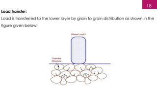
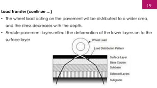
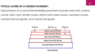
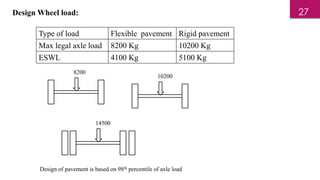
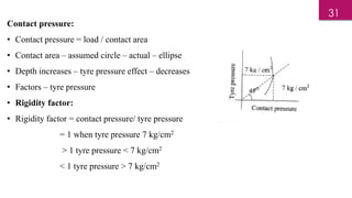
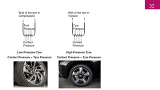
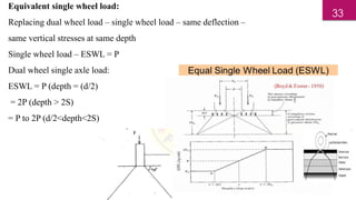
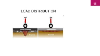
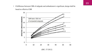
The document provides a comprehensive overview of pavement design, including materials used for flexible and rigid pavements, properties of soil and aggregates, and critical design factors like wheel load and climatic conditions. It discusses various pavement types, their structural differences, and the importance of layer theory in design. Emphasis is placed on characteristics of materials, design methods according to IRC standards, and the performance of highways under different load conditions.

1. Pavement Design: Various properties of highway materials, pavement types, factors to be
considered for pavement design, structural difference between flexible and rigid pavement design.
Flexible pavement design - concept of layer theory, design wheel load, ESWL, EALF. IRC
cumulative standard axles method (IRC - 37: 2013).
Rigid pavement design (IRC 58-2015): Concepts -radius of relative stiffness, Modulus of sub
grade reaction and other characteristics of concrete, wheel load stresses analysis by Westergaards,
temperature stresses and critical combination of stresses. Longitudinal and transverse joints,
contraction joints, expansion joints, construction joints, design of dowel bars and tie bars.
2

2. Materials used in highway construction
Components of highway:
• Embankment or fill
• Subgrade
• Pavement layers of flexible and rigid pavements
If the highway below ground level
Components:
• Prepared cutting
• Subgrade
• Pavement layers of flexible and rigid pavements
Materials for embankment:
• Constructed using locally available soils along the road
Materials in highway cutting:
• Different types of soils along the alignment
3

3. Materials for pavement layers
Flexible pavement layers:
• Granular soils or crushed aggregates or soil-aggregate mixes with adequate
permeability in the drainage layer
• Stone aggregates and fine aggregates in the granular base course
• Coarse aggregates, fine aggregates and bitumen binder in the bituminous
pavement layers in base course or binder course and surface course
4

4. Materials for pavement layers
Rigid pavement layers:
• Granular soils or crushed aggregates or soil-aggregate mixes with adequate
permeability in the drainage layer
• Course aggregates and fine aggregates and Portland cement for the lean
cement concrete in sub base course
• Coarse aggregates, fine aggregates and Portland cement for preparation of
pavement quality concrete in the cement concrete pavement slab serves as
both base and surface course
5

5. Soil
Soil consist mainly of mineral matter formed by the disintegration of rocks, by the action of water,
frost, temperature, pressure or by plant or animal life
Classification: (according to size of particles)
• Gravel
• Sand
• Silt
• Clay
Characteristics depend on
• Size
• Shape
• Surface texture
• Chemical composition
• Electrical charges
6

6. Desirable properties:
• Stability
• Incompressibility
• Permanency of strength
• Minimum changes in volume and stability under adverse
conditions of weather and ground water
• Good drainage
• Ease of compaction
7

7. Aggregates
• Mineral materials such as sand, gravel, and crushed stone
• Aggregate used for base and sub base courses for both flexible and rigid
pavements
Aggregates can be natural or manufactured
Natural aggregates:
• Extracted from larger rock formations through an open excavation (quarry)
• Extracted rock is reduced to usable sizes by mechanical crushing
Manufactured aggregates:
• By product of other manufacturing industries
8

8. Aggregates used in various pavement layers have to bear different
magnitude of stresses due to wheel loads
Aggregates at surface course: resist to
• Wear due to abrasive action of traffic
• Deterioration due to weathering
• Highest magnitude of wheel load stresses
Specifications: depend on
Grain size, shape, texture and its gradation
Sieve analysis – separate different sizes
9

9. Types: based on strength
Hard aggregates:
Wearing course – same properties mentioned previously
Soft aggregates:
Moorum, kankar, laterite, brick aggregates and slag- lower layers of
pavement – low volume traffic
10

10. Desirable properties:
• Strength
• Hardness – resist abrasive action due to moving traffic
• Toughness – resist to impact loads
• Shape of aggregates – flaky and elongated particles will have less strength
• Adhesion with bitumen – less affinity with water compared to bitumen
• Durability – withstand adverse action of weather – soundness (physical and
chemical action of rain and bottom of water, impurities)
• Freedom from deleterious particles – (clean, tough and durable and free from
dust, clay balls, silt, elongated and flat pieces)
11

11. Bitumen
• Binding and water proofing properties
• Low cost
• Bitumen is a black or dark coloured solid or viscous material consist of high
molecular weight hydrocarbons derived from distillation of petroleum or
natural asphalt
• Tar are residues from the destructive distillation of organic substances such as
coal, wood, or petroleum and temperature sensitive
• Bitumen dissolved in petroleum oils
12

12. Requirements of bitumen:
Depend on mix type and construction
• Should not highly temperature susceptible – (hottest weather the mix should
not become too soft or unstable, during cold weather – mix should not
become too brittle causing cracks)
• The viscosity of the bitumen at the time of mixing and compaction should be
adequate.
• Should be adequate affinity and adhesion between the bitumen and
aggregates used in the mix
13

13. 14
Requirements of a pavement
An ideal pavement should meet the following requirements:
• Sufficient thickness to distribute the wheel load stresses to a safe value on the
sub-grade soil,
• Structurally strong to withstand all types of stresses imposed upon it,
• Adequate coefficient of friction to prevent skidding of vehicles,
• Smooth surface to provide comfort to road users even at high speed,
• Produce least noise from moving vehicles,
• Dust proof surface so that traffic safety is not impaired by reducing visibility,
• Impervious surface, so that sub-grade soil is well protected, and
• Long design life with low maintenance cost.

14. A structure consisting of superimposed layers of processed materials above the
natural soil subgrade, whose primary function is to distribute the applied
vehicle loads to the sub-grade.
15

15. Types of Pavements
PAVEMENT
FLEXIBLE PAVEMENT RIGID PAVEMENT
16

16. Flexible pavement:
Flexible pavements are those have low or negligible flexural strength and
flexible in their structural action under load.
17

17. Load transfer:
Load is transferred to the lower layer by grain to grain distribution as shown in the
figure given below;
18

18. Load Transfer (continue …)
• The wheel load acting on the pavement will be distributed to a wider area,
and the stress decreases with the depth.
• Flexible pavement layers reflect the deformation of the lower layers on to the
surface layer
19

19. 20
Types of Flexible Pavements
• Conventional layered flexible pavement
• Full depth asphalt pavement
• Contained rock asphalt mat (CRAM)
Conventional flexible pavements:
• High quality expensive materials placed in the top – stresses are high
• Low quality cheap materials placed in lower layers
Full depth asphalt pavements:
• Placing bituminous layers directly on the soil sub-grade
• Suitable where high traffic and local materials not available
Contained rock asphalt mats:
• Placing dense/open graded aggregate layers in between two asphalt layers
• Modified dense graded asphalt concrete above sub grade will reduce the vertical
compressive strain protect from surface water

20. TYPICAL LAYERS OF A FLEXIBLE PAVEMENT :
Typical layers of a conventional flexible pavement includes seal coat, surface
course, tack coat, binder course, prime coat, base course, sub-base course,
compacted sub-grade, and natural sub-grade.
21

21. TYPICAL LAYERS OF A FLEXIBLE PAVEMENT:
Seal coat is a thin surface treatment used to waterproof the surface and to
provide skid resistance.
Tack coat is a very light application of asphalt emulsion diluted with water. And It
provides bonding between two layers of binder course.
Prime coat is an application of low viscous cutback bitumen to an absorbent
surface like granular bases on which binder layer is placed and provides bonding
between two layers.
22

22. TYPICAL LAYERS OF A FLEXIBLE PAVEMENT (Continue ….)
Surface course is the layer directly in contact with traffic loads and are
constructed with dense graded asphalt concrete.
Binder course purpose is to distribute load to the base course. Binder course
requires lesser quality of mix as compared to course above it.
Base course provides additional load distribution and contributes to the sub-
surface drainage
Sub-base course the primary functions are to provide structural support, improve
drainage, and reduce the intrusion of fines from the sub-grade in the pavement
structure
Sub-grade The top soil or sub-grade is a layer of natural soil prepared to receive
the stresses from the layers above
23

23. FACTORS AFFECTING PAVEMENT DESIGN
1. Design Wheel Load
a. Max. Wheel load
b. Axle configuration
c. Contact pressure
d. ESWL
e. Repetition of loads
2. Climatic Factor
3. Pavement component material
24

24. Design life :
• Number of standard axles – before strengthening of pavement
FP – 10 – 20 yrs, EW – 20, NH and SH – 15, OC – 10-15
RP – 20-30 yrs – HV – 30, LV - 20
Anticipated traffic:
A = P [1+r]n
P = no of commercial vehicles/day
r = traffic growth rate
n = no of years
Example 1: P = 2520 CV/day, r = 7.5%, n = 2 years find A?
Ans: 2912.12 cv/day
25

25. Design Wheel Load.
Max. Wheel load - It is used to determine the depth of the pavement required to
ensure that the subgrade soil does not fail.
Contact pressure - It determines the contact area and the contact pressure
between the wheel and the pavement surface. For simplicity elliptical contact
area is consider to be circular.
26

26. Design Wheel load:
Type of load Flexible pavement Rigid pavement
Max legal axle load 8200 Kg 10200 Kg
ESWL 4100 Kg 5100 Kg
8200
10200
14500
Design of pavement is based on 98th percentile of axle load
27

27. 28

28. Design Wheel Load (Continue)
Axle configuration - the axle configuration is important to know the way in which
the load is applied on the pavement surface.
29

29. 30

30. Contact pressure:
• Contact pressure = load / contact area
• Contact area – assumed circle – actual – ellipse
• Depth increases – tyre pressure effect – decreases
• Factors – tyre pressure
• Rigidity factor:
• Rigidity factor = contact pressure/ tyre pressure
= 1 when tyre pressure 7 kg/cm2
> 1 tyre pressure < 7 kg/cm2
< 1 tyre pressure > 7 kg/cm2
31

31. 32

32. Equivalent single wheel load:
Replacing dual wheel load – single wheel load – same deflection –
same vertical stresses at same depth
Single wheel load – ESWL = P
Dual wheel single axle load:
ESWL = P (depth = (d/2)
= 2P (depth > 2S)
= P to 2P (d/2<depth<2S)
33

33. log 10 ESWL = log10 P + [0.301(log10 (z/(d/2))/(log10 2s/(d/2))]
Assumptions:
Contact area is circle
Influence angle 45 degrees
Soil is homogeneous, elastic, isotropic
Example 2: dual wheel assembly and load on each tyre is 4000 kg. the C/C distance b/w the
tyre is 50 cm, the clear distance b/w tyre is 25 cm. Determine ESWL at a depth of
1) 10 cm,
2) 120 cm,
3) 70 cm , 7185. 55 kg
Ans: Z = 10 cm (d/2 = 25/2 ) =P= 4000
Z = 120 cm = >2S (2x50) =2P = 2x4000 = 8000
ln 10 =
ln 70 =
ln 100 =
ln ESWL = ln 4000 + [(ln 8000-ln 4000)/(ln 100 – ln 10)]*(ln70-ln10)
34

34. Calculate ESWL of a dual wheel assembly carrying 2044 kg each for trail pavement thickness
values of 150, 200 and 250 cm. centre to centre spacing between the two tyres 270 cm and clear
gap between the walls of the tyres 110 cm. 2760, 3000, 3230
35

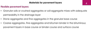
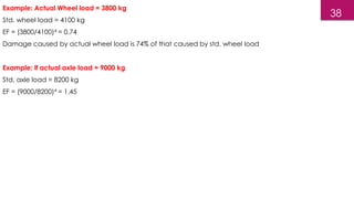
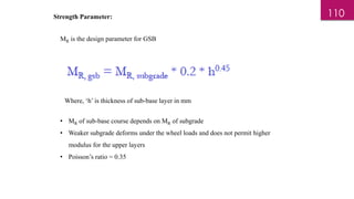
35. Equivalency factor (EF) :
EF = (Actual Wheel load / standard wheel load)4
Gives the % of damage
Example: actual wheel load =3800 kg flexible pavement, standard wheel load = ?
EF = ? 0.74
Example 2: actual axle load = 9000 kg, standard axle load = ? EF = ? 1.45
Example 3: total number of vehicles in terms of standard wheel load? (595 veh/day)
Load range No of veh/day EF
4100 300 1
5200 100 2.59
3800 50 0.74
Standard axle load = [ axle load/8200]4
Tandom axle load = [axle load/14500]4
Total = 300x1+100x2.59+50x0.74
= 595
36

36. 37
Let number of load repetition expected by 80 KN standard axle is 1000, 160 KN is 100 and 40
KN is 10000. Find the equivalent axle load.
S.No Axle load No of load
repetition
EALF
1 40 10000 (40/80)4 = 0.0625 625
2 80 1000 (80/80)4 = 1 1000
3 160 100 (160/80)4 = 16 1600
3225

37. 38
Example: Actual Wheel load = 3800 kg
Std. wheel load = 4100 kg
EF = (3800/4100)4 = 0.74
Damage caused by actual wheel load is 74% of that caused by std. wheel load
Example: if actual axle load = 9000 kg
Std. axle load = 8200 kg
EF = (9000/8200)4 = 1.45

38. 39
Axle load Frequency (%) EF
18 10 23.2
14 20 8.5
10 35 2.212
8 15 0.905
6 20 0.287
Weighted average of EF = (0.1x23.2 + 0.2x8.5+0.35x2.212 + 0.15x0.905+0.2x0.287)/(0.1+0.2+0.35+0.15+0.20)
EF = 5

39. Repetition of loads:
• Each load application causes some deformation and the total deformation is the
summation of all these.
• Although the pavement deformation due to single axle load is very small, the cumulative
effect of number of load repetition is significant.
• Therefore, modern design is based on total number of standard axle load (usually 80 KN
single axle)
• Thickness - Load repetitions and moving wheel loads
• Higher no of repetitions – higher thickness
• Single application of wheel load – deformation small
• Repeated loads – deformation more
• Rate of increase in deformation – very slow – strong pavements
• Very fast – weak pavements
P1N1 = P2N2
Example 1: P1 = 4100 kg, N1 = 6 million, P2 = 8000 kg, N2 = ?
40

40. Climatic Factor
1. Temperature
a) Wide temperature variations may cause damaging effects.
b) Pavement becomes soft in hot weather and brittle in very cold weather.
2. Variation in moisture condition
a) It depends on type of the pavement, type of soil type, ground water
variation etc.
b) It can be controlled by providing suitable surface and subsurface
drainage.
41

41. Characteristic of Pavement material
1. California bearing ratio- It determines the strength of soil sub-grade, sub-base
or base and it is used for the design of pavement.
2. Elastic modulus -It measures the materials resistance to being deformed
elastically upon application of the wheel load.
3. Poisson Ratio – It is the ratio of lateral strain to the axial strain caused by a load
parallel axis along axial strain.
4. Resilient modulus- The elastic modulus based on the recoverable strain under
repeated loads is called the resilient modulus MR =σd /σr .
42

42. 43

43. Characteristic of Pavement material (Continue ….)
• The following material properties are consider for both flexible and rigid
pavements.
• When pavements are considered as linear elastic, the elastic moduli and
poisson’s ratio are specified.
• If the elastic modulus of a material varies with the time of loading, then the
resilient modulus is selected.
44

44. 45

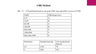
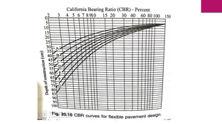
45. Developments in IRC :37-2012
• First published : 1970
• Based on subgrade CBR and traffic in terms of CVPD
• [A: 0-15; B: 15-45; C: 45-150; D: 150-450; E: 450-1500]
• First revision : 1984
• Equivalent Axle Load concept introduced
• Pavement thickness related to cumulative number of standard axle loads
• Up to 30 msa
• Second Revision: 2001
• Up to 150 msa
• Third Revision: 2012
• Usage of new materials and mixtures
46

46. CBR Method
IRC : 37 – 1970 published based on sub grade CBR value and traffic in terms of CVPD
Traffic CBR design curve
0-15 A
15-45 B
45-100 C
150-450 D
450-1500 E
1500-4500 F
More than 4500 G
Penetration Standard load, Kg Unit standard load,
Kg/cm2
2.5 1370 70
5 2055 105

48. 2001 to 2012:
• Huge increase in volume of tandem, tridem and multi-axle vehicles;
heavier axle loads
• New materials and mixtures: stone matrix asphalt, modified bitumen,
foamed bitumen, bitumen emulsion, warm asphalt, cementitious bases
and sub-bases, conventional and chemical soil stabilizers, usage of
local, recycled and engineered marginal aggregates
• Wide usage of these materials in other countries
• Some trial sections using above materials performed well in India
49

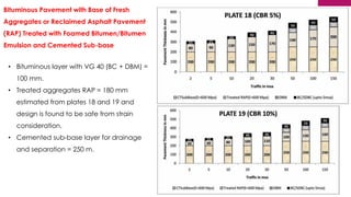
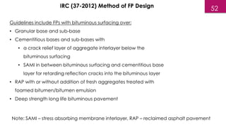
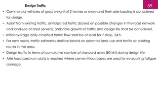
49. • Used to design Flexible Pavements for Expressways, NHs, SHs, MDRs, and other
category of roads with predominant motorized traffic
• Not applicable to low volume roads (ODRs, and VRs) [designed based on
IRC:SP:72-2015]
• Applicable to new pavements.
• IRC:81-1997 {BBD}/IRC:115-2014 {FWD} are used for strengthening existing
pavements
• Design traffic up to 150 msa
IRC (37-2012) Method of FP Design
Note: BBD – benkelman beam deflection, FWD – falling weight deflectometer
50

50. 51
These guidelines do not form a rigid standard and sound engineering judgment considering
the local environment and past pavement performance in the respective regions should be
given due consideration while selecting a pavement composition

51. Guidelines include FPs with bituminous surfacing over:
• Granular base and sub-base
• Cementitious bases and sub-bases with
• a crack relief layer of aggregate interlayer below the
bituminous surfacing
• SAMI in between bituminous surfacing and cementitious base
layer for retarding reflection cracks into the bituminous layer
• RAP with or without addition of fresh aggregates treated with
foamed bitumen/bitumen emulsion
• Deep strength long life bituminous pavement
IRC (37-2012) Method of FP Design
Note: SAMI – stress absorbing membrane interlayer, RAP – reclaimed asphalt pavement
52

52. • Incorporation of design period of more than 15 years
• Computation of effective CBR of subgrade
• Use of rut resistant surface layer
• Use of fatigue resistant bottom bituminous layer
• Selection of surface layer to prevent top down cracking
• Use of bitumen emulsion/foamed bitumen treated RAP in base course
• Consideration of stabilized sub-base and base with locally available soil and aggregates
• Design of drainage layer
• Computation of ESAL considering: (i) single axle with single wheel, (ii) single axle with dual
wheels, (iii) tandem axle, and (iv) tridem axle
• Design of perpetual pavements with deep strength bituminous layer
Guidelines for better performing FPs: 53

53. Flexible Pavement Structure
Water proof, skid resistance
Bond between two
layer of binder
Bond between two layers, water tight surface
54

54. Cross-sectional Elements of a Flexible Pavement
(MORTH, 2001)
Flexible Pavement (MORTH, 2001)
55

55. Flexible Pavement (MORTH, 2013)
Cross-sectional Elements of a Flexible Pavement (MORTH, 2013)
56

56. Cross-sectional Elements of a Flexible Pavement with Dual Carriageway (MORTH, 2013)
Flexible Pavement (MORTH, 2013)
57

57. Treated Shoulders:
•Hard Shoulder: gravel/moorum, any other compacted granular layer or bricks
•Paved Shoulder: bituminous surfacing over granular layers
Flexible Pavement (MORTH, 2013)
58

58. Design Traffic
• Commercial vehicles of gross weight of 3 tonnes or more and their axle loading is considered
for design.
• Apart from existing traffic, anticipated traffic (based on possible changes in the road network
and land-use of area served), probable growth of traffic and design life shall be considered.
• Initial average daily classified traffic flow shall be at least for 7 days, 24 h.
• For new roads, traffic estimates shall be based on potential land-use and traffic on existing
routes in the area.
• Design traffic in terms of cumulative number of standard axles (80 kN) during design life
• Axle load spectrum data is required where cementitious bases are used for evaluating fatigue
damage
59

59. Information required:
• Initial traffic after construction in terms of CVPD
• Traffic growth rate during design life
• Design life
• Spectrum of axle loads
• Vehicle damage factor (VDF)
• Distribution of commercial traffic over the carriageway
60

60. Annual Growth Rate
Estimated from:
• Past trends of traffic growth
• Demand elasticity of traffic w.r.t. macro-economic parameters (GDP or SDP) and expected demand
due to specific developments and land-use changes likely to take place during design life
• If adequate data is not available or if it is less than 5%, 5.0% may be used
61

61. Design Life
• Defined in terms of cumulative number of standard axles in msa that can be carried before a
major strengthening, rehabilitation or capacity augmentation
• National Highways and State Highways, Expressways and Urban Roads: 20 years
• Very high volume roads with design traffic greater than 300 msa and perpetual pavements
can also be designed : 30 years
• Other Categories of Roads: 15 years
• Stage construction (if it is not possible to provide full thickness at the time of pavement
construction):
• thickness of granular layer shall be for full design period
• Not recommended for cemented layers because higher flexural stresses may lead to early
failure
62

62. Vehicle Damage Factor (VDF)
• Multiplier to convert number of commercial vehicles of different axle loads and axle configurations to
the number of standard axle load repetitions
• Defined as equivalent number of standard axles per CV
• Equivalency factor = (axle load/standard axle load)4
Axle type Single wheel or dual wheel Standard axle load
Single
Single 65 KN
Dual 80 KN
Tandom Dual 148 KN
Tridem Dual 224 KN
63

63. Vehicle Damage Factor (VDF)
Sample size for axle load survey:
CVPD Min. CV to be surveyed
<3000 20%
3000 to 6000 15%
> 6000 10%
• Axle load survey shall be performed without any bias for loaded or
unloaded vehicles
• If significant difference in axle loading exists in two directions of traffic,
VDF shall be evaluated direction wise
• Single carriageway with 2 or more lanes shall be designed with same
thickness for the entire carriageway considering the lane with max.
VDF
• For dual carriageways, each direction can have different thickness
64

64. Vehicle Damage Factor (VDF)
Axle load spectrum:
• Spectrum of axle loads shall be determined in terms of axle weights
of single, tandem, tridem axles
• Class intervals shall be 10 kN, 20 kN, and 30 kN for single, tandem,
and tridem axles respectively
• For small sized projects and in absence of sufficient information:
Initial traffic CVPD Terrain
Rolling/ Plain Hilly
0 to 150 1.7 0.6
150 to 1500 3.9 1.7
> 1500 5.0 2.8
65

65. Lane Distribution Factor (LDF)
Single carriageway Dual carriageway
No of lanes LDF No of lanes LDF
Single lane 1 Two lanes 0.75
Two lanes 0.5 Three lanes 0.60
Four lanes 0.4 Four lanes 0.45
66

66. where, N = cumulative number of standard axles, msa
A = initial traffic in the year of completion of construction (in CVPD)
D = LDF
F = VDF
n = design life, years
r = annual growth rate of commercial vehicles
67
cumulative number of standard axles

67. where, P = number of commercial vehicles as per last count
x = number of years between the last count and the year of completion of
construction
68

68. 69
Two lane carriage way
Initial traffic in the year of completion of construction = 400 CVPD (sum of both directions)
Traffic growth rate = 7.5 %
Design life = 15 years
Vehicle damage factor based on axle load survey = 2.5 standard axle per commercial vehicle
Compute CSA.
Ans: 7.2msa

69. 70
4 lane divided carriage way
Initial traffic in each direction = 5640 cvpd
Design life = 10
Traffic growth rate = 8%
Axle load using the road = 11800kg
Find CSA
LDF = 0.75
VDF = (11800/8160)4 = 4.5
r=0.08
N = 100msa

70. • FP modeled as elastic multilayer structure
• Compute stresses and strains at critical locations
Principles of Pavement Design
71

71. • Series of interconnected cracks caused by fatigue failure of HMA surface under repeated traffic loading
• In thin pavements, crack initiates at the bottom of the HMA layer where the tensile stress is high and
propagates to the surface as one or more longitudinal cracks (Bottom-up cracks!!!)
Principles of Pavement Design fatigue criteria
• In thick pavements, the cracks initiate from
the top in areas of high localized tensile
stresses resulting from tyre-pavement
interaction and asphalt binder aging (Top-
down cracks!!!)
Note: HMA – hot mix asphalt
72

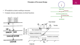
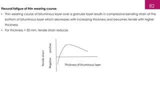
72. • Tensile strain near surface close to edge of a wheel results in longitudinal cracking followed by
transverse cracking before flexural cracking if mix tensile strength is not adequate at high
temperatures [tensile strain in wearing course near edge of tyre can be higher than that at bottom of
bituminous layer at higher temperatures]
• High tensile strength at higher temperatures can delay top down cracking (using VG40/PMB/CRMB
binders)
• Wearing course must also be fatigue resistant in addition to being rut resistant (high modulus mix)
Principles of Pavement Design
Note: PMB – polymer modified bitumen, CRMB – crumb rubber modified bitumen
73

73. 74

74. 75
Fatigue in Bottom Bituminous Layer:
• Fatigue life is defined as the number of load repetitions to 20% cracking for traffic up to 30 msa and 10%
beyond 30 msa
• Formulated two fatigue equations using pavement performance data collected from all corners of
India
• First case: computed strains in 80% of the actual data in the scatter plot were higher than the limiting
strains predicted by the model and termed as 80% reliability level
• Second case: corresponds to 90% reliability level
Principles of Pavement Design

75. Reliability: (AASHTO-1993)
• Reliability is a means of incorporating some degree of certainty into the design process to
ensure that various design alternatives will last the analysis period; reliability level to be
used for design shall increase as the volume of traffic increases
• Analysis period: time period that any design strategy must cover
Reliability levels for various functional classifications (AASHTO-1993)
Functional classification Urban Rural
Interstate and other freeways 85-99.9 80-99.9
Principal arterials 80-99 75-95
Collectors 80-95 75-95
Local 50-80 50-80
The reliability of the pavement design-performance process is the probability that a pavement section
designed using the process will perform satisfactorily over the traffic and environmental conditions for the
design period
76

76. Fatigue cracking criteria for bituminous layer 77

77. • Mixes used in pavements for which performance data collected in India were designed for an average
4.5% air voids (min. 3% to max. 6%) and an average 4.5% bitumen content (min. 4% to max. 5%
depending upon gradation and specific gravity of aggregates) by weight of the mix (11.5% by volume)
• In order to take into account the effect or air voids (Va) and volume of bitumen (Vb), “C” factor is used
in fatigue models
• Slight changes in Va and Vb will have huge impact on fatigue life
• Target for low air voids and higher bitumen content for the lower bituminous layer to obtain fatigue
resistant mix
78

78. Substituting Va = 4.5% and Vb = 11.5% in the above equation results in the first equation
79

79. Substituting Va = 4.5% and Vb = 11.5% in the above equation results in the first equation
80

80. Effect of air voids and volume of bitumen on Nf
81

81. Flexural fatigue of thin wearing course:
• Thin wearing course of bituminous layer over a granular layer results in compressive bending strain at the
bottom of bituminous layer which decreases with increasing thickness and becomes tensile with higher
thickness
• For thickness > 50 mm, tensile strain reduces
82

82. 83
Resilient Modulus of Bituminous Mixes, MPa:
• Poisson‟s ratio is 0.35 is recommended for temperatures up to 35 C, and 0.50 for higher temperatures

83. 84
Temperature of Bituminous Surface:
• MR and Poisson‟s ratio depends on temperature
• Average Annual Air Temperature (AAAT) collected from Indian Meteorological Department:
S.No City AAAT (°C)
1 Mumbai 27.10
2 Guwahati 23.87
3 Hyderabad 26.16
4 New Delhi 24.53
5 Chennai 27.97
6 Kharagpur 28.16

84. 85
Average Monthly Air Temperature (AMAT), Average Monthly Pavement Temperature (AMPT)

85. 86
Cementitious sub base and base
• Cementitious materials crack due to shrinkage and temperature changes even
without loading
• Slow setting cementitious materials with low cement content develop fine
cracks and are preferred over high cement content mixes producing wider
cracks
• Recommended elastic modulus of cementitious layers is much lower than the
laboratory determined UCC value (Unconfined compression test)

86. Fatigue Cracking in Cementitious Layers:
• Cement treated layers fatigue cracking addressed in two levels:
• Thickness of cemented layer is evaluated from fatigue consideration in
terms of cumulative standard axles
• Cumulative fatigue damage due to individual axles is calculated based on
stress ratio
• Cumulative fatigue damage of all wheels should be less than 1 during the
design life of pavement
• If greater than 1, pavement section has to be revised
• Second level analysis is necessary when very heavy traffic is operating on the
highways
87

87. Fatigue life in terms of standard axles
12
Where, RF = reliability factor for cementitious materials for failure against fatigue (=1 for
Expressways, NHs, and other heavy volume roads; = 2 for other roads carrying less than
1500 trucks per day)
N = fatigue life of the cementitious material
E = elastic modulus of cementitious material
ƹt = tensile strain in the cementitious layer, (µstrain; µm/m)
88

88. Fatigue equation for cumulative damage analysis:
Where, Nfi = fatigue life in terms of cumulative number of axle load of class “i”
σt = tensile stress under cementitious base layer
MRup = 28 day flexural strength of the cementitious base
• Fatigue criterion is considered satisfied if Ʃ(Ni/Nfi) is less than 1, where Ni is actual no.
of axles of axle load of class “i"
• Tandem and tridem axles can be taken as equivalent to 2 and 3 single axles, respectively
because stresses due to axles located at distances more than 1.30 m apart do not overlap
89

89. Rutting:
• Rutting is the permanent deformation in pavement occurs longitudinally
along the wheel path
• Rutting is caused by deformation in the subgrade and other non-
bituminous layers
• Bituminous mixes also undergo rutting due to secondary compaction and
shear deformation under heavy traffic load and higher temperature
(controlled by proper mix design)
• Rutting is limited to 20 mm in 20% of the length for design traffic up to 30
msa and 10% of the length for the design traffic beyond 30 msa
• Mixes using higher viscosity grade bitumen or modified bitumen will resist
rutting
90

90. Subgrade rutting criteria
• Surface depression in the wheel path; pavement uplift (shearing) may occur along the sides
of the rut
• Ruts are particularly evident after a rain when they are filled with water (hydroplaning); can
be hazardous because ruts tend to pull a vehicle towards the rut path as it is steered across
the rut
• Caused due to permanent deformation in any of the
pavement layers or subgrade usually caused by
vertical compression or consolidation or lateral
movement of the materials due to traffic loading
91

91. 92
Similar to fatigue criteria, formulated two rutting equations using the pavement
performance data collected from all corners of India (80 and 90% reliability
levels)

92. Subgrade
• Top 500 mm portion of the roadway.
• Heavy compaction recommended for Expressways, NHs, SHs, and MDRs.
• Shall be compacted to 97% of dry density achieved with heavy compaction.
• CBR at most critical moisture conditions likely to occur in the field (general practice: 4 days soaking).
• Soaking for 4 days may be unrealistic severe field moisture condition.
• For example, if climate is arid throughout the year (annual rainfall < 1000 mm) and water table is too
deep to affect the subgrade adversely.
• Results in conservative design if 4 days soaking is adopted.
93

93. 94
In such cases, CBR shall be determined at natural moisture content of the soil at subgrade depth
immediately after recession of the monsoon.
In-situ CBR of subgrade from DCP (Dynamic Cone Penetrometer):

94. • Subgrade CBR values varies along road alignment even on a homogeneous section.
• 90 percentile CBR is recommended
• Example:
• Following are 16 CBR values for a road alignment: 3.5, 5.2, 8.0, 6.8, 8.8, 4.2, 6.4, 4.6, 9.0, 5.7, 8.4, 8.2, 7.3,
8.6, 8.9, 7.6
• Arrange in ascending order: 3.5, 4.2, 4.6, 5.2, 5.7, 6.4, 6.8, 7.3, 7.6, 8.0, 8.2, 8.4, 8.6, 8.8, 8.9, 9.0
• Calculate percentage ≥each of the values:
• For CBR of 3.5%, percentage of values ≥ 3.5 = 100
• For CBR of 4.2%, percentage of values ≥ 4.2 = 93.75
95

95. • 90th percentile CBR = 4.7%
• 80th percentile CBR = 5.7%
96

96. • AI recommends 87.5 percentile subgrade modulus for design traffic > 1 msa
• For very large data, CBR values can be grouped for homogeneous sections and adopt above
procedure
• Subgrade with different soil types: min. 6 to 8 avg. CBR values (avg. of 3 tests) for each soil type along
road alignment for determination of design CBR
• 90th percentile is adopted as design CBR value (90 percent of avg. CBR values are design value) for
high volume roads (Expressways, NHs, and SHs)
• Other category roads: 80th percentile is design CBR value
97

97. 98
• Pavement design shall be based on CBR value of the weakest subgrade soil over a given section of the
road
• Pavement thickness may be modified with change in subgrade soil but may not be practically possible.
• At least three samples shall be tested on each type of soil at the same density and moisture content
• If variation is more than above values, design CBR shall be the average of test results from at least six
samples
Subgrade
CBR, % Max. variation in CBR
<5 ±1
5 to 10 ±2
11 to 30 ±3
>30 ±5

98. • If difference between CBR of subgrade and embankment is significant, design shall be
based on effective CBR
(IRC: 37-2012)
99

99. Resilient Modulus (MR) of Subgrade 100

100. 101
Expansive Soils as Subgrade
• Use of expansive clay is not allowed for subgrade.
• If unavoidable, following procedure shall be adopted.
• Expansive soils (black cotton soils, montmorillonite clays) are characterized by
extreme hardness and deep cracks when dry and tendency to heave during
wetting.
• Moisture changes due to seasonal wetting and drying causes volumetric
changes and leads to pavement distortion, cracking, and unevenness.
• Volume changes in these soils depends on (i) dry density of compacted soil,
(ii) moisture content, and (iii) structure of soil and method of compaction.

101. 102
Expansive Soils as Subgrade
• Expansive soils swell very little when compacted at low densities and high
moisture content; recommended to compact the soils to slightly wet of
OMC (+1 to 2%).
• Thickness design shall be based on 4-day soaked CBR. • Field density = 95%
of laboratory density Buffer Layer:
• Buffer layer made of non-expansive cohesive soil cushion of 0.6 to 1.0 m
thickness:
I. prevents ingress of water into the underlying expansive soil,
II. counteracts swelling and if the underlying expansive soil heaves,
movement will be more uniform.

102. 103
• If buffer layer is not economically feasible, blanket course made of suitable
material and thickness shall be provided.
Blanket Course:
• At least 225 mm thickness.
• Composed of coarse/medium sand (or) non-plastic moorum with PI <5%.
• Provided above expansive soil to serve as sub-base.
• Extended over entire formation width.
• Alternatively, lime-stabilized black cotton sub-base extending over entire
formation width may be provided together with measures for efficient
drainage.
• Improvement of drainage can significantly reduce the magnitude of seasonal
heaves.

103. 104
Drainage Measures:
• Provision must be made for lateral drainage of the pavement section.
• Granular sub-base/base shall be extended across the shoulders.
• Camber of 1:40 for BT surface and cross-slope of 1:20 for berms to shed-off
surface run-off quickly.
• Standing water not allowed on either side of embankment.
Expansive Soils as Subgrade

104. 105
Drainage Measures:
• Min. height of 1 m (0.6 m for existing road without history of being overtopped)
between subgrade level and highest water level shall be ensured.
• 40 mm thick BT surfacing shall be provided to prevent ingress of water through
surface.
• Shoulders shall be made of impervious material.
• Lime stabilized black cotton soil shoulder of 150 to 200 mm thickness is an
economical option.
• Example problem related to “Drainage Layer Design” would be discussed in
IRC:58-2015

105. 106
Sub-base and base layers can be unbound (granular) or chemical stabilized with cement, lime fly-ash and
other stabilizers Different layers of a flexible pavement:
Pavement Composition

106. 107
• For pavements with cementitious base, a crack relief layer is provided between bituminous layer and
cementitious base
• Crack relief layer (100 mm WMM or SAMI)considerably delays reflection crack in bituminous layer
• Base layer may also consist of:
i. granular materials treated with bitumen emulsion or foamed bitumen,
ii. fresh aggregates or aggregates obtained from reclaimed asphalt pavements (RAP) treated with
foamed bitumen or bitumen emulsion
iii. Unbound base layer may consist of WMM or WBM
• Sub-base layer serves three function:
i. Protects subgrade from overstressing,
ii. Provides a platform for construction traffic, and
iii. Serves as drainage and filter layer.
Pavement Composition

107. Unbound Sub-Base Course
• Materials: natural sand, moorum, gravel, laterite, kankar, brick metal, crushed stone, crushed slag, reclaimed crushed CC, RAP
or combinations of these meeting requirements of MoRTH specifications for roads and bridge works (MoRTH, 2013)
• Three gradations each are specified for close and coarse graded granular sub-base materials
• Material passing 425 µm shall have liquid limit less than 25% (LL<25%) and plasticity index less than 6% (PI<6%)
• Materials shall satisfy specifications to meet strength, filter, and drainage requirements of the layer
108

108. Sub-base shall consist of two layers:
• Lower layer forms separation/filter layer to prevent intrusion of subgrade soil into the pavement
• Upper layer acts as drainage layer (drains water entering through cracks, shoulders, or median)
• Drainage layer shall be tested for permeability (gradation can be altered to ensure required permeability)
• Design filter layer and drainage layer using IRC:SP:42-1994 and IRC:SP:50-1999
• Minimum thickness of GSB layer:
• Minimum thickness of drainage and filter layer shall be 100 mm each
• Minimum thickness of the single filter cum drainage layer shall be 150 mm
109

109. Strength Parameter:
MR is the design parameter for GSB
Where, ‘h’ is thickness of sub-base layer in mm
• MR of sub-base course depends on MR of subgrade
• Weaker subgrade deforms under the wheel loads and does not permit higher
modulus for the upper layers
• Poisson’s ratio = 0.35
110

110. Bound Sub-Base Course
• Materials: soil, aggregate or soil aggregate mixture modified with chemical stabilizers such as cement, lime-fly-ash, and
commercially available stabilizers
• Sub-base drainage layer may consist of coarse graded aggregates bound with 2 to 3% cement while retaining permeability
• Geosynthetics can be used to improve permeability for cement treated sub-base course
• Strength Parameter:
• Elastic modulus (E) determined from Unconfined Compressive Strength (UCS) is the design parameter for bound sub-base
course
• For cementitious granular sub-base (CGSB) with 7-day UCS of 1.5 to 3 MPa:
• Where, UCS is 28 day strength of CGSB
• Design E is 600 MPa, and µ is 0.25
• •For stabilized sub-bases with 7-day UCS of 0.75 to 1.5 MPa, recommended design E is 400 MPa, µ is 0.25
111

111. Unbound Base Course
• May consist of:
• WMM
• WBM
• CRM
• Reclaimed CC, etc.
• When both base and sub-base are made of unbound layers, composite MR of granular sub-base and base is:
Where, ‘h’ is combined thickness of sub-base and base layers in mm
Poisson’s ratio of granular base and sub-base is 0.35
Note: CRM – crumb rubber modifier, CC – crushed concrete
112

112. Cementitious Base Course
• Consists of aggregates or soils or both stabilized with chemical stabilizers such as cement, lime, lime-fly-ash or other
stabilizers with minimum strength of 4.5 to 4.7 MPa in 7 or 28 days
• Cement shall attain this strength in 7 days
• Lime or lime-fly-ash stabilized granular materials and soils shall attain this strength in 28 days
• Initial modulus of cementitious bases are in the range of 10,000 to 15,000 MPa and long term modulus may be taken as 50%
of initial modulus due to shrinkage cracks and construction traffic
113

113. Strength Parameter
• Flexural strength is required for carrying out fatigue analysis as per fatigue
equation
• Modulus of rupture for chemically stabilized bases is taken as 20% of the 28 day
UCS
• Cementitious stabilized aggregates: 1.40 Mpa
• Lime-fly-ash soil: 1.05 Mpa
• Soil cement: 0.70 Mpa
• Poisson’s ratio of cemented layers: 0.25
114

114. Durability Criteria
• Minimum cementitious material in the cementitious base layer shall be such that in a wetting drying test, loss of weight of
the stabilized material shall not exceed 14% after 12 cycles
• In cold and snow bound regions (Ar. P., J.K., H.P., etc.) durability shall be determined by freezing and thawing tests and loss
of weight of the stabilized material shall not exceed 14% after 12 cycles
• Cementitious layer meeting strength requirements are expected to meet the durability criteria
115

115. Crack Relief Layer
• SAMI using elastomeric modified bitumen provided over cementitious layer delays cracks propagating into bituminous
layers
• 100 mm WMM sandwiched between bituminous layer and cementitious layer is more effective in arresting crack
propagation
• Shoving and deformation caused in unbound layer due to the construction traffic can be minimized by treating with 1 to 2%
bitumen
Note: WMM – wet mix macadam, SAMI – stress absorbing membrane interlayer
116

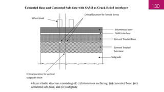
116. 117
Crack Relief Layer (SAMI) •
• Interlayers designed to dissipate energy by deforming horizontally and vertically, allowing the movement
(vertical/horizontal) of underlying layers without causing large tensile stresses in bituminous overlay
• Barksdale, 1991: SAMI is a soft layer [flexible!] (usually thin) used to reduce tensile stress in the overlay in
the vicinity of the crack in the underlying old layer and absorb stress
• Lytton, 1989:
• Crack starts to propagate (due to thermal and traffic loading) from its original position upward until it
reaches the stress-relieving layer. Due to its low stiffness, the interlayer will exhibit large deformations
resulting in dissipation of energy. The crack propagation will stop for a while due to lack of energy, and
then propagate from the top of the interlayer upward to the surface (bottom-up cracking)
• In the second failure mode, crack starts to propagate from its original position upward until it reaches the
stress-relieving layer. The crack then begins from the top of the overlay to the interlayer (top-down
cracking)

117. Crack Relief Layer (SAMI)
• Geotextiles
• Modified binder
• Sand asphalt
• Impregnated glass fibre
• Geogrids
• Interlayer stress absorbing geocomposite
• Bitumen-impregnated glass fibre
• Steel reinforced nettings
• Bituminous membrane
• Bituminous mixtures consisting of high polymer modified asphalt content (7 to 7.5% by weight)
118

118. Modulus of Crack Relief Layer
• MR of good quality granular layer provided between cementitious and bituminous layers depends on the confinement pressure
• MR may vary from 250 to 1000 MPa and 450 MPa is used in analysis of pavements
• Strong support from cementitious base results in higher MR
• Poisson‟s ratio: 0.35
119

119. 120
Resilient Modulus of Granular Materials
Shall be determined from repeated load triaxial test

120. 121
Resilient or Elastic Modulus of Aggregate Interlayer
Cementitious Base Course
Material description Modulus over
uncracked
cemented layer
(Mpa)
Recommended
modulus (Mpa)
Poisson’s ratio
High quality graded crushed rock (WMM) 250 to 1000 450 0.35
Graded crushed stone and soil binder; PI<6 200 to 800 350 0.35
Natural gravel; PI<6;CBR>80% 100 to 600 300 0.35

121. Bitumen Emulsion/Foamed Bitumen Treated Aggregates/RAP Base Course
• Design MR= 600 MPa (Laboratory MR = 600 to 1200 MPa)
• Above values can be ensured if indirect tensile strength of 100 mm diameter Marshall specimen of emulsion or foamed
bitumen treated material has a min. 100 kPa in wet condition and 225 kPa in dry condition under 50 mm/min. rate of loading
at 25º C
• Poisson’s ratio = 0.35
122

122. Bituminous Layers
MR of Bituminous Mixes, MPa
µ= 0.35 up to 35 ºC and 0.50 above 35 ºC
123

123. 124
Bituminous Layers
Selection of Binder
Maximum
average air
temperature
Traffic (CVPD) Bituminous
course
Grade of bitumen to be used
≤ 30 ≤ 1500 CVPD BM, DBM and
BC
VG 10/VG20
<40 For all types of
traffic
BM, DBM, SDBC
and BC
VG30
≥ 40 Heavy loads,
expressways
msa>30msa
DBM, SDBC, BC VG40 bitumen for wearing course as
well as binder course, modified bitumen
may be used for the wearing course
30 and 40 degrees

124. Perpetual Pavement
• Pavement with life ≥50 years, ≥ 300 msa
• Bituminous layer never cracks if tensile strain caused by traffic < 70 µm/m
• Little rutting if vertical subgrade strain < 200 µm/m
• Different layers are designed and constructed such that only surface layer is renewed
from time to time
125

125. Pavement Design
• Bar charts for traffic ranging from 2 to 150 msa
• For traffic below 2msa: IRC:SP:72-2015
• City roads shall be designed for min. 2 msa
126
• Thickness design for traffic between 2 and 30 msa is same as IRC:37-2001
• In all cases of cementitious sub-bases (cases 2, 3, and 4), top 100 mm thickness of sub-base shall be
porous and shall act as drainage layer

126. Pavement Design
Five combinations of traffic and material properties:
1. Granular base and granular sub-base
2. Cementitious base and cementitious sub-base of aggregate interlayer for crack
relief (upper 100 mm of cementitious sub-base is the drainage layer)
3. Cementitious base and cementitious sub-base with SAMI at the interface of base
and the bituminous layer
4. Foamed bitumen or bitumen emulsion treated RAP or fresh aggregates over 250
mm cementitious sub-base
5. Cementitious base and granular sub-base with crack relief layer of aggregate
above the cementitious base
127

127. Granular Base and Granular Sub-base
• Considered as a 3 layer elastic structure consisting of: (i) bituminous surfacing, (ii)
granular base and sub-base, and (iii) subgrade
128

128. Cemented Base and Cemented Sub-base with Crack Relief Aggregate Interlayer
• 5 layer elastic structure consisting of: (i) bituminous surfacing, (ii) aggregate
interlayer, (iii) cemented base, (iv) cemented sub-base, and (v) subgrade
129

129. Cemented Base and Cemented Sub-base with SAMI as Crack Relief Interlayer
4 layer elastic structure consisting of: (i) bituminous surfacing, (ii) cemented base, (iii)
cemented sub-base, and (iv) subgrade
130

130. Foamed Bitumen or Bitumen Emulsion Treated RAP or Aggregates Over Cemented
Sub-base
4 layer elastic structure consisting of: (i)
bituminous surfacing, (ii) treated RAP base,
(iii) cemented sub-base, and (iv) subgrade
131

131. Cemented Base and Granular Sub-base with Crack Relief Aggregate Interlayer
5 layer elastic structure consisting of: (i)
bituminous surfacing, (ii) aggregate interlayer,
(iii) cemented base, (iv) granular sub-base, and
(v) subgrade
132

132. 133
Design the pavement for construction of a new flexible pavement with the following
data:
• Four lane divided carriage way
• Initial traffic in the year of completion of construction = 5000 CVPD (sum of both
directions)
• % of single, tandem and tridem axles are 45%, 45% and 10% respectively
• Traffic growth rate per annum = 6.0
• Design life = 20 years
• Vehicle damage factor = 5.2
• CBR of soil below the 500mm of the subgrade = 3%
• CBR of the 500mm of the subgrade from the borrow pits = 10%

133. 134
• LDF = 0.75
• Initial traffic = 2500 CVPD assuming 50% in each direction
• VDF = 5.2
• CSA = 131 msa
Lane Distribution Factor (LDF)
Single carriageway Dual carriageway
No of lanes LDF No of lanes LDF
Single lane 1 Two lanes 0.75
Two lanes 0.5 Three lanes 0.60
Four lanes 0.4 Four lanes 0.45

134. 135
CBR of the embankment material = 3%
CBR of 500mm of subgrade = 10%
Effective CBR of the subgrade = 7%
Design resilient modulus of the compacted subgrade = 17.6 x (7)0.64 = 62MPa

135. 136
Thickness of granular layers:
WMM = 250 mm,
GSB = 230 mm
DBM = 130mm
BC = 50mm
Granular base and sub base
Resilient modulus of granular layer = 0.2 x (480)0.45 x 62 = 200 Mpa.

136. 137
Cemented base and cemented sub base with
aggregate inter layer of 100mm
Design traffic as above 131 msa.
• Bituminous layer with VG 40 (BC + DBM) =
100 mm.
• Aggregate interlayer = 100 mm.
• Cemented base = 120 mm ((thickness of
the cemented base for CBR 5 and 10 are
130 mm and 100 mm respectively).
• Cemented sub-base layer for drainage
and separation = 250 mm

137. 138
Cemented Base and Cemented Sub-base with
Sami Layer Over Cemented Base
• Bituminous layer with VG 40 (BC +
DBM) = 100 mm.
• Cemented base = 165 mm estimated
from the plates 14 and 15 for
cumulative fatigue damage analysis
• Cemented sub-base layer for
drainage and separation = 250 m.

138. 139
Bituminous Pavement with Base of Fresh
Aggregates or Reclaimed Asphalt Pavement
(RAP) Treated with Foamed Bitumen/Bitumen
Emulsion and Cemented Sub-base
• Bituminous layer with VG 40 (BC + DBM) =
100 mm.
• Treated aggregates RAP = 180 mm
estimated from plates 18 and 19 and
design is found to be safe from strain
consideration.
• Cemented sub-base layer for drainage
and separation = 250 m.

139. 140
Bituminous Pavement with Cemented Base and Granular Sub-base with 100 mm WMM Layer Over
Cemented Base
• BC (VG 40) = 50 mm,
• DBM (VG 40) = 50 mm,
• WMM = 100 mm,
• cemented base = 195 mm estimated
from plates 22 and 23 for fatigue
damage analysis,
• GSB = 250 mm.

140. 141
Rigid pavement design

141. 142
• The pavements which possess flexural strength, are
called as rigid pavements.
• The rigid pavements are generally made of Portland
cement concrete and some times called as ‘CC
Pavements’.
• The cement concrete used for rigid pavements is
called as ‘Pavement Quality Concrete (PQC)’.
• The rigid or CC pavements are designed and
constructed for a design life of 30 years.

142. 143
Rigid pavements are usually provided under the
circumstances:
• Very heavy rainfall
• Poor soil conditions
• Poor drainage
• Extreme climatic conditions
• Combination of some of these conditions
which may lead to development of cracks in
pavements.

143. 144
The components of rigid pavement from
bottom to top consists of
• Soil subgrade
• Granular sub-base course
• Base course
• CC/PQC pavement slab

144. 145
Modulus of sub-grade reaction
Westergaard considered the rigid pavement slab as a thin elastic plate resting on soil sub-
grade, which is assumed as a dense liquid.
The upward reaction is assumed to be proportional to the deflection.
Base on this assumption, Westergaard defined a modulus of sub-grade reaction K in kg/cm3
given by
K = p /∆
where ∆ is the displacement level taken as 0.125 cm and
p is the pressure sustained by the rigid plate of 75 cm diameter at a deflection of 0.125 cm.

145. 146
Relative stiffness of slab to sub-grade
• A certain degree of resistance to slab deflection is offered by the sub-grade.
• The sub-grade deformation is same as the slab deflection.
• Hence the slab deflection is direct measurement of the magnitude of the sub-grade pressure.
• This pressure deformation characteristics of rigid pavement lead Westergaard to the define the
term radius of relative stiffness l in cm is given by the equation
where E is the modulus of elasticity of cement concrete in kg/cm2 (3.0×105 ), µ is the Poisson’s
ratio of concrete (0.15), h is the slab thickness in cm and K is the modulus of sub-grade
reaction.

146. 147
Compute the radius of relative stiffness of 15cm thick cement concrete slab using the following data:
Modulus of elasticity of cement concrete = 2.1 x 105 kg/cm2
Poisson’s ratio for concrete = 0.15
Modulus of subgrade reaction, K = (a) = 3.0 kg/cm3, (b) = 7.5 kg/cm3
1) l = 67.0cm
2) l = 53.3cm

147. 148
Critical positions of loading:
• Since the pavement slab has finite length and width, either the character or the intensity of
maximum stress induced by the application of a given traffic load is dependent on the
location of the load on the pavement surface.
• There are three typical locations namely the interior, edge and corner, where differing
conditions of slab continuity exist.
• These locations are termed as critical load positions.

148. 149
Equivalent radius of resisting section:
When the interior point is loaded, only a small area of the pavement is resisting the
bending moment of the plate. Westergaard’s gives a relation for equivalent radius of
the resisting section in cm in the equation
where a is the radius of the wheel load distribution in cm and h is the slab thickness in cm.

149. 150
Compute the equivalent radius of resisting section of 20cm thick slab, given that the
radius of contact area wheel load is 15cm
h = 20cm, a = 15
a/h = 15/20 = 0.75<1.724
b = 14.07cm

150. 151
Wheel load stresses - Westergaard’s stress equation
• The cement concrete slab is assumed to be homogeneous and to have uniform elastic
properties with vertical sub-grade reaction being proportional to the deflection.
• Westergaard developed relationships for the stress at interior, edge and corner regions,
denoted as σi , σe, σc in kg/cm2 respectively and given by the equation
where h is the slab thickness in cm, P is the wheel load in kg, a is
the radius of the wheel load distribution in cm, l the radius of the
relative stiffness in cm and b is the radius of the resisting section in
cm

151. 152
• Due to corner loading, tensile stress is developed on the top of the pavement across
the corner bisector or the diagonal.
• If the corner load stress exceeds the flexural strength of the CC slab a crack is likely to
develop a cross diagonal on the top surface of the pavement.
• Maximum stress produced by a wheel load at corner does not exit around the load,
but it occurs at some distance X along the diagonal.
X = 2.58 𝑎𝑙

152. 153
Using the data given below, calculate the wheel load stresses at
a. Interior
b. Edge and
c. Corner regions of a cement concrete pavement using Westergaard’s stress equations. Also
determine the probable location where the crack is likely to develop due to corner loading
Wheel load, P = 5100kg
Modulus of elasticity of cement concrete, E = 3.0 x 105 kg/cm2
Pavement thickness, h = 18cm
Poisson’s ratio of concrete = 0.15
Modulus of subgrade reaction, K = 6.0 kg/cm3
Radius of contact area, a = 15cm
l = 70.6cm, b = 14.0cm
σi = 19.3
σe = 28.54
σc = 24.27, X = 84cm

153. 154
Temperature stresses:
Temperature stresses are developed in cement concrete pavement due to variation in slab
temperature. This is caused by
(i) daily variation resulting in a temperature gradient across the thickness of the slab and
(ii) seasonal variation resulting in overall change in the slab temperature.
The former results in warping stresses and the later in frictional stresses

154. 155
Wrapping stresses:
Due to temperature differential between the top and bottom of the pavement as a
result of daily variation in temperature at the location.
The warping stress at the interior, edge and corner regions, denoted as σti , σte , σtc in kg/cm2
respectively and given by the equation
where E is the modulus of elasticity of concrete in kg/cm2 (3×105 ),
є is the thermal coefficient of concrete per oC (1×10−7 ) t is the
temperature difference between the top and bottom of the slab,
Cx and Cy are the coefficient based on Lx/l in the desired
direction and Ly/l right angle to the desired direction, µ is the
Poisson’s ration (0.15), a is the radius of the contact area and l is
the radius of the relative stiffness.

155. 156

156. 157
Determine the warping stresses at interior, edge and corner of a 25cm thick cement concrete
pavement with transverse joints at 5.0m interval and longitudinal joints at 3.6m intervals. The
modulus of subgrade reaction, K is 6.9 kg/cm3 and radius of loaded area is 15cm. Assume
maximum temperature differential during day to be 0.6 degrees per cm slab thickness (for
warping stresses at interior and edge) and maximum temperature differential of 0.4 degrees/cm
slab thickness during the night (for warping stress at the corner). Additional data are given
below:
e = 10x10-6 per degree
E = 3x105 kg/cm2
Poisson’s ratio=0.15

157. 158
h = 25cm
a = 15cm
Lx = 500cm
Ly = 360cm
t1 = 0.6 x 25 = 15
t2 = 0.4x25 = 10
l = 87.2cm
Lx/l = 5.73, Cx = 0.88
Ly/l = 4.13, Cy = 0.54
σti , σte , σtc are 22.15, 19.8, 4.88 kg/cm2

158. 159
Frictional stresses:
• Due to temperature rise and fall in cement concrete slab, expansion and contraction of the slab
• Slab movements restrained with the supporting layer below with the frictional force
• Total force developed in the cross section due to movement of half the length of the slab (Lc/2) and
frictional resistance due to restraint at the interface in half the slab length
Sf x h x b x (100kg) = b x (Lc/2) x (h/100) x W x f
Sf = (W x Lc x f)/(2x104)
Where
Sf = stress developed due to inter-face friction in cement concrete pavement /unit area (kg/cm2)
W = unit weight of concrete, kg/cm3
f = coefficient of friction at the interface
Lc = spacing between the contraction joint, m
b = slab width, m

159. 160
The spacing between the contraction joints of a CC pavement is 4.2m. Determine the tensile
stress developed in the CC pavement due to contraction if the coefficient of friction between
the bottom of the pavement and the supporting layer is 1.1 and the unit weight of CC is 2400
kg/cm3
Given L = 4.2m, f=1.1 and W = 2400
Sf = (W x Lc x f)/(2x104)
= (2400x4.2x1.1)/(2x104)
= 0.554 kg/cm2

160. 161

161. 162

162. 163
Combination of stresses:
The cumulative effect of the different stress give rise to the following thee critical cases
Summer, mid-day:
The critical stress is for edge region given by σcritical = σe + σte − σf
= load stress + warping stress – frictional stress
Winter, mid-day:
The critical combination of stress is for the edge region given by σcritical = σe +σte +σf
= load stress + warping stress + frictional stress
Mid-nights:
The critical combination of stress is for the corner region given by σcritical = σc + σtc
= load stress + warping stress

163. 164

164. 165
•Joints are the discontinuities in the concrete pavement slab, and help to release stresses due to
temperature variation, subgrade moisture variation, shrinkage of concrete etc.
•There are various types of joints in concrete pavement, e.g. contraction joint, construction joint,
expansion joint and warping joint.
Contraction joint: Contraction joints are provided along the transverse direction to take care of
the contraction of concrete slab due to its natural shrinkage.
•The purpose of the contraction joints is to allow the contraction of the slab due to fall in slab
temperature below the construction temperature.
The design considerations are:
The movement is restricted by the sub –grade friction
Design involves the length of the slab given by
Where Sc allowable stress, W unit weight, f coefficient of sub-grade friction
Joints

165. 166
• Steel reinforcements can be use, however with a maximum spacing of 4.5m as per IRC.

166. 167
Expansion joint:
• Expansion joints are provided along the transverse direction to allow movement (expansion/
contraction) of the concrete slab due to temperature and subgrade moisture variation.
• The purpose of the expansion joint is to allow the expansion of the pavement due to rise in
temperature with respect to construction temperature. The design consideration are:
• Provided along the longitudinal direction.
• Design involves finding the joint spacing for a given expansion joint thickness subjected to
some maximum spacing.

167. 168
Construction joint:
Construction joints are provided whenever the construction work stops temporarily. The joint
direction could be either along the transverse or longitudinal direction.
Warping joint:
Warping joints are provided along the longitudinal direction to prevent warping of the concrete
slab due to temperature and subgrade moisture variation.
These discontinuities (joints) could be extended to the full or partial depth of the slab.

168. 169

169. 170
Dowel bars:
The purpose of the dowel bar is to effectively transfer the load between two concrete slabs and
to keep the two slabs in same height. The dowel bars are provided in the direction of the traffic
(longitudinal). The design considerations are:
• Mild steel rounded bars,
• bonded on one side and free on other side

170. 171
Bradbury’s analysis:
Bradbury’s analysis gives load transfer capacity of single dowel bar in shear, bending
and bearing as follows:
where, P is the load transfer capacity of a single dowel bar in shear s, bending f and bearing b, d
is the diameter of the bar in cm, Ld is the length of the embedment of dowel bar in cm, δ is the
joint width in cm, Fs, Ff, Fb are the permissible stress in shear, bending and bearing for the dowel
bar in kg/cm2 .

171. 172
Design procedure
Step 1:
Find the length of the dowel bar embedded in slab Ld
Step 2:
Find the load transfer capacities Ps, Pf , and Pb of single dowel bar with the Ld
Step 3:
Assume load capacity of dowel bar is 40 percent wheel load, find the load capacity factor f as

172. 173
Step 4:
Spacing of the dowel bars.
• Effective distance upto which effective load transfer take place is given by 1.8 l, where l is the
radius of relative stiffness.
• Assume a linear variation of capacity factor of 1.0 under load to 0 at 1.8 l.
• Assume a dowel spacing and find the capacity factor of the above spacing.
• Actual capacity factor should be greater than the required capacity factor.
• If not, do one more iteration with new spacing.

173. 174
Example Design size and spacing of dowel bars at an expansion joint of concrete pavement of
thickness 25 cm. Given the radius of relative stiffness of 80 cm. design wheel load 5000 kg. Load
capacity of the dowel system is 40 percent of design wheel load. Joint width is 2.0 cm and the
permissible stress in shear, bending and bearing stress in dowel bars are 1000,1400 and 100
kg/cm2 respectively.

174. 175
Given, P = 5000 kg, l = 80 cm,
h = 25 cm, δ = 2 cm, Fs = 1000
kg/cm2 , Ff = 1400 kg/cm2 and
Fb = 100 kg/cm2 ; and assume
d = 2.5 cm diameter.
Step-1: length of the dowel bar Ld

175. 176

176. 177
Tie bars:
In contrast to dowel bars, tie bars are not load transfer devices, but serve as a means to tie two
slabs. Hence tie bars must be deformed or hooked and must be firmly anchored into the
concrete to function properly. They are smaller than dowel bars and placed at large intervals.
They are provided across longitudinal joints.
Step 1: Diameter and spacing: The diameter and the spacing is first found out by equating the total sub-
grade friction tot he total tensile stress for a unit length (one meter). Hence the area of steel per one meter
in cm2 is given by:

177. 178
where, b is the width of the pavement panel in m, h is the depth of the pavement in cm, W is the unit weight
of the concrete (assume 2400 kg/cm2 ), f is the coefficient of friction (assume 1.5), and Ss is the allowable
working tensile stress in steel (assume 1750 kg/cm2 ). Assume 0.8 to 1.5 cm φ bars for the design.
Step 2 Length of the tie bar: Length of the tie bar is twice the length needed to develop bond stress equal
to the working tensile stress and is given by:
where, d is the diameter of the bar, Ss is the allowable tensile stress in kg/cm2 , and Sb is the allowable bond
stress and can be assumed for plain and deformed bars respectively as 17.5 and 24.6 kg/cm2.

178. 179
A cement concrete pavement of thickness 18 cm, has two lanes of 7.2 m with a joint. Design the
tie bars.
Given h=18 cm, b=7.2/2=3.6m, Ss = 1750 kg/cm2 W = 2400 kg/cm2 f = 1.5 Sb = 24.6 kg/cm2.

179. 180
1. Design size and spacing of dowel bars at an expansion joint of concrete pavement of
thickness 20 cm. Given the radius of relative stiffness of 90 cm. design wheel load 4000 kg.
Load capacity of the dowel system is 40 percent of design wheel load. Joint width is 3.0 cm
and the permissible stress in shear, bending and bearing stress in dowel bars are 1000,1500
and 100 kg/cm2 respectively.
2. Design the length and spacing of tie bars given that the pavement thickness is 20cm and
width of the road is 7m with one longitudinal joint. The unit weight of concrete is 2400 kg/m3 ,
the coefficient of friction is 1.5, allowable working tensile stress in steel is 1750 kg/cm2 , and
bond stress of deformed bars is 24.6 kg/cm2 .