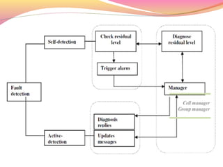
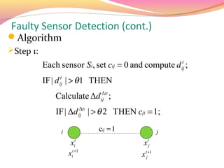
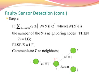
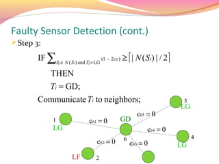
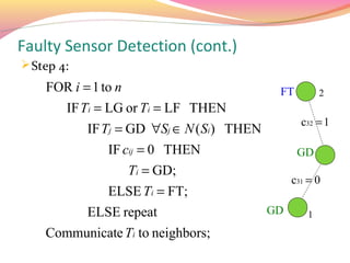
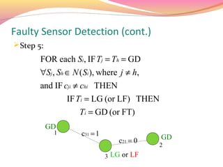
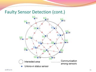
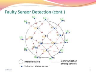
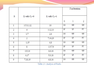
Presented By:
    Pavithra R.
     III M C A
Mangalore University
CONTENTS
 •   INTRODUCTION TO WSN
 •   FAULT MANAGEMENT MECHANISM FOR WSN
 •   FAULT DETECTION AND DIAGNOSIS
 •   FAULT RECOVERY
 •   NETWORK AND FAULT MODEL
 •   FAULTY SENSOR DETECTION
 •   CONCLUSION
 •   FUTURE SCOPE
INTRODUCTION
A wireless sensor network is a collection of sensor nodes
      organized into a cooperative network
  •   WSN are used to collect data from the environment.
  •   A sensor network consists of multiple detection
      stations called sensor nodes, each of which is small,
      lightweight and portable.
  •   The nodes in the network are connected via Wireless
      communication channels.
  •   Each node has capability to sense data, process the
      data and send it to rest of the nodes or to Base
      Station.
  •   These networks are limited by the node battery
      lifetime.
Every sensor node is equipped with a transducer,
 microcomputer, transceiver and power source.
The transducer generates electrical signals based on
 sensed physical effects and phenomena. The
 microcomputer processes and stores the sensor output.
The transceiver, which can be hard-wired or wireless,
 receives commands from a central computer and
 transmits data to that computer. The power for each
 sensor node is derived from the electric utility or from a
 battery.
Wireless sensor networks (WSN) usually have limited
 energy and transmission capacity, which can't match the
 transmission of a large number of data collected by
 sensor nodes.
WSN ARCHITECTURE


                                         Sensor Node

                                         Gateway


                                         Base Station

  Wireless Sensor Network Architecture
Fault Management Mechanism for WSN
In this approach a new fault management mechanism
 was proposed to deal with fault detection and recovery.
It proposes a hierarchical structure to properly distribute
 fault management tasks among sensor nodes by heavily
 introducing more self-managing functions.
The proposed fault management mechanism can be
 divided into two phases:

   Fault detection and diagnosis
   Fault recovery
Fault Detection and Diagnosis
Detection of faulty sensor nodes can be achieved by two
 mechanisms i.e. self-detection (or passive-detection) and
 active-detection.
In self-detection, sensor nodes are required to
 periodically monitor their residual energy, and identify the
 potential failure.
In this scheme, we consider the battery depletion as a
 main cause of node sudden death. A node is termed as
 failing when its energy drops below the threshold value.
Self-detection is considered as a local computational
 process of sensor nodes, and requires less in-network
 communication to conserve the node energy.
To efficiently detect the node sudden death, fault
 management system employed an active detection
 mode.
In active detection, cell manager asks its cell members
 on regular basis to send their updates. Such as the cell
 manager sends “get” messages to the associated
 common nodes on regular basis and in return nodes
 send their updates. This is called in-cell update cycle.
The update_msg consists of node ID, energy and
 location information.
The exchange of update messages takes place between
 cell manager and its cell members. If the cell manager
 does not receive an update from any node then it sends
 an instant message to the node .
If cell manager does not receive the acknowledgement in
 a given time, it then declares the node faulty and passes
 this information to the remaining nodes in the cell.
Fault Recovery
After nodes failure detection (as a result of self-detection
 or active detection), sleeping nodes can be awaked to
 cover the required cell density or mobile nodes can be
 moved to fill the coverage hole.
A cell manager also appoints a secondary cell manager
 within its cell to acts as a backup cell manager. Cell
 manager and secondary cell manager are known to their
 cell members.
If the cell manager energy drops below the threshold
 value (i.e. less than or equal to 20% of battery life), it
 then sends a message to its cell members including
 secondary cell manager.
This is an indication for secondary cell manager to stand
 up as a new cell manager and the existing cell manager
 becomes common node and goes to a low computational
 mode.
Common nodes will automatically start treating the
 secondary cell manager as their new cell manager and
 the new cell manager upon receiving updates from its cell
 members; choose a new secondary cell manager.
The failure recovery mechanisms are performed locally
 by each cell.
Figure: Virual Grid of Nodes
Network model and Fault model
Sensors are randomly deployed in the interested area
 which is very dense and all the sensors have a common
 transmission range.
Depending on majority voting among the sensors, we
 assume that each sensor node has at least 3 neighboring
 nodes.
Because a large amount of sensors are deployed into the
 interested area to form a wireless network, this condition
 can be easily obtained.
Each sensor node is able to locate its neighbors within its
 transmission range via a broadcast/ acknowledge
 protocol. Faults can occur at different levels of the sensor
 network such as system software, hardware, physical
 layer, and middleware.
In this mechanism, we focus on hardware level faults by
 assuming all system software as well as the application
 software is always fault tolerant.
We can categorize the hardware components of sensor
 nodes into two groups.
The first group of hardware level components consists of
 a storage subsystem, computation engine and power
 supply infrastructure.
The second groups of components are sensors and
 actuators.
Sensor nodes are still capable of receiving, sending, and
 processing when they are faulty in the algorithm.
Faulty Sensor Detection
Definition:
n : total number of sensors;
p : probability of failure of a sensor;
k : number of neighbor sensors;
S : set of all the sensors;
N ( Si ) : set of the neighbors of Si;
xi : measurement of Si;
   t
d ij : measurement difference between Si and Sj at time t ,
  d ij = xit − x tj ;
     t
Faulty Sensor Detection (cont.)
 Δtl = tl + 1 − tl;
 Δd ij tl : measurement difference between Si and Sj from
     Δ


    time tl to tl + 1, Δd ij tl = d ijl +1 − d ijl = ( xitl +1 − x tjl +1 ) − ( xitl − x tjl );
                           Δ         t          t


 cij : test between Si and Sj , cij ∈{0, 1}, cij = cji;
θ1 and θ 2 : two predefined threshold values;
Ti : tendency value of a sensor, Ti ∈{LG, LF, GD, FT};
Faulty Sensor Detection (cont.)
Algorithm
Step 1:
           Each sensor Si, set cij = 0 and compute d ij ;
                                                      t


           IF | d ij | > θ 1 THEN
                   t


               Calculate Δd ij tl ;
                             Δ


               IF | Δd ij tl | > θ 2 THEN cji = 1;
                        Δ


                 i            cij = 1               j
                      xit                   x tj
                     xit +1                x tj+1
Faulty Sensor Detection (cont.)
 Step 2:

    IF ∑Sj ∈ N ( Si ) cij ≤  | N ( Si ) | /2 , where | N ( Si ) | is
    the number of the Si ' s neighboring nodes THEN
         Ti = LG;
    ELSE Ti = LF;
    Communicate Ti to neighbors;                                 2

                                                    c42 = 1
                                           LF
                     1
                               c41 = 1
                                                 c43 = 0
                                             4                   3
Faulty Sensor Detection (cont.)
 Step 3:

        IF ∑Sj ∈ N ( Si ) and Tj = LG (1 − 2 cij ) ≥  | N ( Si ) | / 2
              THEN
          Ti = GD;
        Communicate Ti to neighbors;                                        5
                                                                           LG
                                                        c65 = 0
               1                c61 = 0         GD
               LG                                            c64 = 0
                                                 6                              4
                                    c62 = 0          c63 = 0               LG
                        LF          2
Faulty Sensor Detection (cont.)
 Step 4:
    FOR i = 1 to n                            FT          2
      IF Ti = LG or Ti = LF THEN
                                                    c32 = 1
            IF Tj = GD ∀Sj ∈ N ( Si ) THEN
               IF cij = 0 THEN                     GD
                   Ti = GD;
                                                  c31 = 0
              ELSE Ti = FT;
            ELSE repeat                      GD       1

    Communicate Ti to neighbors;
Faulty Sensor Detection (cont.)
 Step 5:
        FOR each Si, IF Tj = Th = GD
        ∀Sj , Sh ∈ N ( Si ), where j ≠ h,
        and IF cji ≠ chi THEN
                 IF Ti = LG (or LF) THEN
                     Ti = GD (or FT)
            GD
             1       c31 = 1                 GD
                                   c21 = 0
                                             2
                               3 LG or LF
Faulty Sensor Detection (cont.)
                            LG                       LG                        LG
                  LG
                                        0        0            1            1
                        1
                                    LG                            LF
                                                 0            1        0                   LG
                                    0                                                  1
                                                                        LF
             LG        LG                        LG
                   0                             1            0        1           1
                                        1                                                  LG
                                1           LF            1       LG           0
                                            0                 0
                                LF                   1                 1
                  LG        0                1
                                                  LG               1           LG
                                        1        0            0
                                    LG
                                                              LG


2008/10/01                                                                                      23
Faulty Sensor Detection (cont.)
                            LG                     LG                         LG
                  LG
                                     0         0            1             1
                        1
                                 GD                             FT
                                                                 LF
                                               0            1         0                   LG
                                 0                                                    1
                                                                      FT
                                                                       LF
             LG        GD                      GD
                   0                           1            0         1           1
                                     1                                                    LG
                             1           FT
                                          LF            1       GD            0
                                          0                 0
                             FT
                              LF                   1                  1
                  LG        0              1
                                                GD                1           LG
                                     1         0            0
                                 LG
                                                            LG


2008/10/01                                                                                     24
CONCLUSION
In a faulty sensor detection algorithm where each sensor
 identifies its own status to be either ”good” or ”faulty” and
 the claim is then supported or reverted by its neighbors
 as they also evaluate the node behavior.
The probabilities of faulty sensors being diagnosed as
 “good” and good sensors not being diagnosed as “good”
 are very low.
Future Scope
In future we intend to calculate the detection accuracy for
  the nodes in the Wireless Sensor Network where
  detection accuracy depicts the ratio of the number of
  faulty sensors detected to the total number of faulty
  sensors in the network. The time consumed by approach
  to find out the faulty node is relatively less. So we want to
  verify it for larger number of nodes.
TH ANK YO U

FAULT DETECTION IN WIRELESS SENSOR NETWORK

  • 1.
    Presented By: Pavithra R. III M C A Mangalore University
  • 2.
    CONTENTS • INTRODUCTION TO WSN • FAULT MANAGEMENT MECHANISM FOR WSN • FAULT DETECTION AND DIAGNOSIS • FAULT RECOVERY • NETWORK AND FAULT MODEL • FAULTY SENSOR DETECTION • CONCLUSION • FUTURE SCOPE
  • 3.
    INTRODUCTION A wireless sensornetwork is a collection of sensor nodes organized into a cooperative network • WSN are used to collect data from the environment. • A sensor network consists of multiple detection stations called sensor nodes, each of which is small, lightweight and portable. • The nodes in the network are connected via Wireless communication channels. • Each node has capability to sense data, process the data and send it to rest of the nodes or to Base Station. • These networks are limited by the node battery lifetime.
  • 4.
    Every sensor nodeis equipped with a transducer, microcomputer, transceiver and power source. The transducer generates electrical signals based on sensed physical effects and phenomena. The microcomputer processes and stores the sensor output. The transceiver, which can be hard-wired or wireless, receives commands from a central computer and transmits data to that computer. The power for each sensor node is derived from the electric utility or from a battery. Wireless sensor networks (WSN) usually have limited energy and transmission capacity, which can't match the transmission of a large number of data collected by sensor nodes.
  • 5.
    WSN ARCHITECTURE Sensor Node Gateway Base Station Wireless Sensor Network Architecture
  • 6.
    Fault Management Mechanismfor WSN In this approach a new fault management mechanism was proposed to deal with fault detection and recovery. It proposes a hierarchical structure to properly distribute fault management tasks among sensor nodes by heavily introducing more self-managing functions. The proposed fault management mechanism can be divided into two phases:  Fault detection and diagnosis  Fault recovery
  • 7.
    Fault Detection andDiagnosis Detection of faulty sensor nodes can be achieved by two mechanisms i.e. self-detection (or passive-detection) and active-detection. In self-detection, sensor nodes are required to periodically monitor their residual energy, and identify the potential failure. In this scheme, we consider the battery depletion as a main cause of node sudden death. A node is termed as failing when its energy drops below the threshold value. Self-detection is considered as a local computational process of sensor nodes, and requires less in-network communication to conserve the node energy. To efficiently detect the node sudden death, fault management system employed an active detection mode.
  • 8.
    In active detection,cell manager asks its cell members on regular basis to send their updates. Such as the cell manager sends “get” messages to the associated common nodes on regular basis and in return nodes send their updates. This is called in-cell update cycle. The update_msg consists of node ID, energy and location information. The exchange of update messages takes place between cell manager and its cell members. If the cell manager does not receive an update from any node then it sends an instant message to the node . If cell manager does not receive the acknowledgement in a given time, it then declares the node faulty and passes this information to the remaining nodes in the cell.
  • 10.
    Fault Recovery After nodesfailure detection (as a result of self-detection or active detection), sleeping nodes can be awaked to cover the required cell density or mobile nodes can be moved to fill the coverage hole. A cell manager also appoints a secondary cell manager within its cell to acts as a backup cell manager. Cell manager and secondary cell manager are known to their cell members. If the cell manager energy drops below the threshold value (i.e. less than or equal to 20% of battery life), it then sends a message to its cell members including secondary cell manager.
  • 11.
    This is anindication for secondary cell manager to stand up as a new cell manager and the existing cell manager becomes common node and goes to a low computational mode. Common nodes will automatically start treating the secondary cell manager as their new cell manager and the new cell manager upon receiving updates from its cell members; choose a new secondary cell manager. The failure recovery mechanisms are performed locally by each cell.
  • 12.
  • 13.
    Network model andFault model
  • 14.
    Network model andFault model Sensors are randomly deployed in the interested area which is very dense and all the sensors have a common transmission range. Depending on majority voting among the sensors, we assume that each sensor node has at least 3 neighboring nodes. Because a large amount of sensors are deployed into the interested area to form a wireless network, this condition can be easily obtained. Each sensor node is able to locate its neighbors within its transmission range via a broadcast/ acknowledge protocol. Faults can occur at different levels of the sensor network such as system software, hardware, physical layer, and middleware.
  • 15.
    In this mechanism,we focus on hardware level faults by assuming all system software as well as the application software is always fault tolerant. We can categorize the hardware components of sensor nodes into two groups. The first group of hardware level components consists of a storage subsystem, computation engine and power supply infrastructure. The second groups of components are sensors and actuators. Sensor nodes are still capable of receiving, sending, and processing when they are faulty in the algorithm.
  • 16.
    Faulty Sensor Detection Definition: n: total number of sensors; p : probability of failure of a sensor; k : number of neighbor sensors; S : set of all the sensors; N ( Si ) : set of the neighbors of Si; xi : measurement of Si; t d ij : measurement difference between Si and Sj at time t , d ij = xit − x tj ; t
  • 17.
    Faulty Sensor Detection(cont.) Δtl = tl + 1 − tl; Δd ij tl : measurement difference between Si and Sj from Δ time tl to tl + 1, Δd ij tl = d ijl +1 − d ijl = ( xitl +1 − x tjl +1 ) − ( xitl − x tjl ); Δ t t cij : test between Si and Sj , cij ∈{0, 1}, cij = cji; θ1 and θ 2 : two predefined threshold values; Ti : tendency value of a sensor, Ti ∈{LG, LF, GD, FT};
  • 18.
    Faulty Sensor Detection(cont.) Algorithm Step 1: Each sensor Si, set cij = 0 and compute d ij ; t IF | d ij | > θ 1 THEN t Calculate Δd ij tl ; Δ IF | Δd ij tl | > θ 2 THEN cji = 1; Δ i cij = 1 j xit x tj xit +1 x tj+1
  • 19.
    Faulty Sensor Detection(cont.)  Step 2: IF ∑Sj ∈ N ( Si ) cij ≤  | N ( Si ) | /2 , where | N ( Si ) | is the number of the Si ' s neighboring nodes THEN Ti = LG; ELSE Ti = LF; Communicate Ti to neighbors; 2 c42 = 1 LF 1 c41 = 1 c43 = 0 4 3
  • 20.
    Faulty Sensor Detection(cont.)  Step 3: IF ∑Sj ∈ N ( Si ) and Tj = LG (1 − 2 cij ) ≥  | N ( Si ) | / 2 THEN Ti = GD; Communicate Ti to neighbors; 5 LG c65 = 0 1 c61 = 0 GD LG c64 = 0 6 4 c62 = 0 c63 = 0 LG LF 2
  • 21.
    Faulty Sensor Detection(cont.)  Step 4: FOR i = 1 to n FT 2 IF Ti = LG or Ti = LF THEN c32 = 1 IF Tj = GD ∀Sj ∈ N ( Si ) THEN IF cij = 0 THEN GD Ti = GD; c31 = 0 ELSE Ti = FT; ELSE repeat GD 1 Communicate Ti to neighbors;
  • 22.
    Faulty Sensor Detection(cont.)  Step 5: FOR each Si, IF Tj = Th = GD ∀Sj , Sh ∈ N ( Si ), where j ≠ h, and IF cji ≠ chi THEN IF Ti = LG (or LF) THEN Ti = GD (or FT) GD 1 c31 = 1 GD c21 = 0 2 3 LG or LF
  • 23.
    Faulty Sensor Detection(cont.) LG LG LG LG 0 0 1 1 1 LG LF 0 1 0 LG 0 1 LF LG LG LG 0 1 0 1 1 1 LG 1 LF 1 LG 0 0 0 LF 1 1 LG 0 1 LG 1 LG 1 0 0 LG LG 2008/10/01 23
  • 24.
    Faulty Sensor Detection(cont.) LG LG LG LG 0 0 1 1 1 GD FT LF 0 1 0 LG 0 1 FT LF LG GD GD 0 1 0 1 1 1 LG 1 FT LF 1 GD 0 0 0 FT LF 1 1 LG 0 1 GD 1 LG 1 0 0 LG LG 2008/10/01 24
  • 26.
    CONCLUSION In a faultysensor detection algorithm where each sensor identifies its own status to be either ”good” or ”faulty” and the claim is then supported or reverted by its neighbors as they also evaluate the node behavior. The probabilities of faulty sensors being diagnosed as “good” and good sensors not being diagnosed as “good” are very low.
  • 27.
    Future Scope In futurewe intend to calculate the detection accuracy for the nodes in the Wireless Sensor Network where detection accuracy depicts the ratio of the number of faulty sensors detected to the total number of faulty sensors in the network. The time consumed by approach to find out the faulty node is relatively less. So we want to verify it for larger number of nodes.
  • 28.