Download to read offline


![Application Of Affine Theorem To Orthotropic Rectangular Reinforced Concrete Slab With Long Side.
DOI: 10.9790/1684-1303023038 www.iosrjournals.org 38 | Page
References
[1] Johansen, K.W., “Yield-Line Theory “, Cement and Concrete Association, London, 1962, pp. 181.
[2] Goli, H B. and Gesund, H., “Linearity in Limit State Design of Orthotropic Slabs” J. of Structural Division, ASCE,, Oct.1979,
Vol.105, No. ST10, pp.1901-1915.
[3] Rambabu, K. and Goli, H B. “Simplified approach to design orthogonal slabs using affine theorem”, Journal of Structural
Engineering, Chennai, India, Dec 2006-Jan 2007,Vol.33,No.5, pp.435-442.
[4] Islam, S. and Park, R., “Yield line analysis of two-way reinforced concrete slabs with openings”, The Structural Engineer, June
1971, Vol. 49, No. 6, pp. 269-275.
[5] Zaslavsky. Aron, Yield line analysis of rectangular slabs with central opening”, Proc. Of ACI, December 1967, Vol. No.64, pp.
838-844.
[6] Siva Rama Prasad, Ch., and Goli, H. B., “Limit State Coefficients for Orthogonal Slabs.” International Journal of Structural
Engineering, India, Jan-June 1987, Vol.7, No.1, pp. 93-111.
[7] Sudhakar, K.J., and Goli, H B., “Limit State Coefficients for Trapezoidal- Shaped Slabs Supported on Three Sides”, Journal of
Structural Engineering, Chennai, India, June-July 2005, Vol.32, No.2, pp.101-108.
[8] Veerendra Kumar and Milan Bandyopadhyay “ Yield line analysis of two way reinforced concrete slabs having two adjacent edges
discontinuous with openings” ,Journal of Structural Engineering, Chennai, India, June-July 2009,Vol.36,No.2, pp.82-99.
[9] “Indian Standard Plain and Reinforced Concrete-Code of Practice”, IS 456:2000, BIS New Delhi
Notations:
Continuous edge
Simply supported edge
Free edge
Negative yield line
CS A slab supported on all sides continuously (restrained)
I1 and I2 Negative moment coefficients in their corresponding directions
I1mult Negative ultimate yield moment per unit length provided by top tension
Reinforcement bars placed parallel to x-axis.
I2mult Negative ultimate yield moment per unit length provided by top tension
Reinforcement bars placed parallel to y-axis.
K1
xmult Positive ultimate yield moment per unit length provided by bottom tension
Bars placed parallel to X-axis
K1
ymult Positive ultimate yield moment per unit length provided by bottom tension
Bars placed parallel to Y-axis
K1
x
y
K
K
'
'
K2
yK
I
'
2
Lx, Ly Slab dimensions in X and Y directions respectively
mult Ultimate Yield moment per unit length of the slab
r Aspect ratio of slab defined by Lx/Ly.
r1, r2, r3, r4 Non dimensional parameters of yield line propagation
SS A slab simply supported on all sides
TLC A slab restrained on two long edges and other two sides simply supported
TSC A slab restrained on two long edges and other two sides simply supported
udl Uniformly Distributed Load
Wult Ultimate uniformly distributed load per unit area of slab.
α, β coefficients of opening in the slab
μ Coefficient of orthotropy
2
1
IK
IK
y
x
'
'](https://image.slidesharecdn.com/f1303023038-160728091532/85/F1303023038-9-320.jpg)

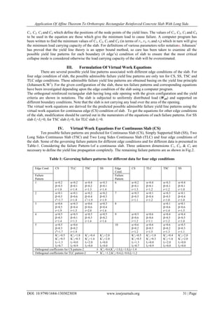
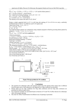
This document presents an analysis of orthotropic reinforced concrete slabs with long side openings using the affine theorem and yield line method. Ten possible yield line failure patterns are considered for slabs with continuous, simply supported, two long sides continuous, and two short sides continuous edge conditions. Virtual work equations are formulated for each failure pattern. Numerical examples are provided to illustrate the governing failure patterns for different slab geometries and support conditions. The affine theorem is used to transform orthotropic slab properties into equivalent isotropic properties to simplify the analysis.