1) The document describes the design of an automatic landing system for unmanned aerial vehicles that accounts for ground effect. 2) A gain scheduling approach is used where linear models derived from the nonlinear aircraft model are used to design PID controllers for different phases of flight. Gains are scheduled based on altitude to account for changing aerodynamic coefficients. 3) The system controls airspeed and glide slope throughout landing for simplicity. Ground effect is modeled to obtain aerodynamic coefficients as a function of altitude from out-of-ground effect to in-ground effect.

1. International Journal of Engineering Inventions
e-ISSN: 2278-7461, p-ISSN: 2319-6491
Volume 4, Issue 6 (November 2014) PP: 44-51
www.ijeijournal.com Page | 44
Gain scheduling automatic landing system by modeling
Ground Effect
Caterina Grillo1
, Fernando Montano2
Department DICGIM, University of Palermo, Italy
Abstract: Taking ground effect into account a longitudinal automatic landing system is designed. Such a
system will be tested and implemented on board by using the Preceptor N3 Ultrapup aircraft which is used as
technological demonstrator of new control navigation and guidance algorithms in the context of the “Research
Project of National Interest” (PRIN 2008) by the Universities of Bologna, Palermo, Ferrara and the Second
University of Naples.
A general mathematical model of the studied aircraft has been built to obtain non–linear analytical
equations for aerodynamic coefficients both Out of Ground Effect and In Ground Effect. To cope with the strong
variations of aerodynamic coefficients In Ground Effect a modified gain scheduling approach has been
employed for the synthesis of the controller by using six State Space Models. Stability and control matrices have
been evaluated by linearization of the obtained aerodynamic coefficients. To achieve a simple structure of the
control system, an original landing geometry has been chosen, therefore it has been imposed to control the same
state variables during both the glide path and the flare.
Keywords: Automatic landing, gain scheduling, ground effect, UAS
I. INTRODUCTION
In spite of a number of potentially valuable civil UAS applications The International Regulations
prohibit UAS from operating in the National Air Space. Maybe the primary reasons are safety concerns. In fact
their ability to respond to emergent situations involving the loss of contact between the aircraft and the ground
station poses a serious problem. Therefore, to an efficient safe insertion of UAS in the Civil Air Transport
System one important element is their ability to perform automatic landing afterwards the failure. At the present,
a few number of UAS is fully autonomous from takeoff to landing [1]. Moreover, the mathematical model of
ground effect is usually neither included in the model of the aircraft during takeoff and landing nor in the design
requirements of the control system [1], [2], [3], [4]. Some authors take into account the ground effect using a
mean value of down-wash angle [5]. To cope with strong variation of aerodynamic characteristics most of
papers make use of two different mathematical models of the aircraft during landing: the first Out the Ground
Effect (OGE) and the second In Ground Effect (IGE).
Besides for an automatic longitudinal landing control, two different control systems are used: a glide
path control system during the glide slope phase and a flare control system in order to execute the flare
maneuver [2], [3], [4] [5]. Usually ,during the glide slope glide path angle, pitch attitude and air speed are
controlled [2], [3], [4] .Other authors use normal acceleration, air speed and pitch rate [5]. A lot of paper
employees altitude and descent velocity. Recently, because of either GPS use or the increase of sensor’s
performances for the angular rates measurement, pitch angle and pitch rate are often used [2], [3], [6], [7], [8].
Sometimes, instead of airspeed (V) , because of the small values of the glide slope angle, aircraft velocity along
the longitudinal axes (u) and elevation are controlled and the altitude is employed to tune the control laws[9]. As
the airplane gets very close to the runway threshold, the glide path control system is disengaged and the flare
control system is engaged. This one controls either the vertical descent rate of the aircraft, or the air speed and
altitude [2], [3], [4], [5]. To control height accurately in the presence of wind and gust the perpendicular
distance and velocity from the required flight path are used to calculate a demanded maneuver acceleration, this
one, by means of aircraft speed and orientation is converted to pitch rate [10].
Obviously the above mentioned approach leads to a complex structure of the control system, therefore
it could give rise to significant system errors due to unmodelled ground effect. To overcome these complexities,
the objective of this paper is the design of a longitudinal control system having the following characteristics:
a. The controlled variables are the same during both the glide path and the flare;
b. According to previous papers [11], [12]; the aerodynamic coefficient vs. altitude are modeled during takeoff
instead of using a mean value [13], [14];
c. Indirect flight path control is carried out by controlling the velocity vector (Airspeed V and glide path angle
γ).

2. Automatic Landing System for Civil Unmanned Aerial System
www.ijeijournal.com Page | 45
Item a. allows to achieve a simple structure of the control system independently of the actual flight
phases. Item b. permits to take into account the actual ground effect. Item c. implies that the elevator and the
throttle control the velocity vector, during the whole path.
Because of high angles of attack during landing, a nonlinear mathematical model of the aircraft should
be used for designing the controller [15], [16]. As a consequence, to obtain satisfactory performance, nonlinear
controllers should be developed [17]. To overcome the difficulties due to the use of nonlinear models of the
aircraft in ground effect, a gain scheduling flight control system has been designed using the following
approach:
 The Landing flight path has been divided into two segments: the glide path for aircraft altitudes h >of the
wing span b (OGE) and the flare for h <= b (IGE);
 The flare manoeuvre starts for h = b;
 An acceptable number of linear models has been obtained by means of linearization of the original
nonlinear model in various flight conditions: one in OGE condition (from 300 ft to h = b) and five in IGE
conditions (during flare). (These ones are necessary to employ the linearization through the small
disturbance theory).
 A modified gain scheduling approach has been employed for the synthesis of the controller. Initially, by
using the obtained linear models, various PID controllers have been designed. Afterwards the obtained PID
gains have been modelled by using analytical equations, taking into account the hyperbolic variations of the
aerodynamic coefficients. Finally, by linearization of the obtained equation for the gains a set of control
gains matrix has been calculated.
 A flight control system has been implemented consisting of the above PID controllers and a supervisor
which schedules one of them to be inserted online, depending on the actual flight condition.
The contributions of this paper are: the general model of the aerodynamic coefficients in the whole
range of altitude from OGE to IGE condition, the original landing geometry, the simple structure of the control
system. Therefore, the system is easily configurable since to control the velocity vector only a small set of
sensors are necessary. In fact, by using both Inertial Measurement Unit (IMU) and air data boom, pitch attitude
(ϑ), airspeed (V) and angle of attack (AOA, α) are easy obtainable. Otherwise a low rate GPS may be used to
obtain glide path angle (γ) airspeed (V) and vertical ground speed (VZ).
II. FLIGHT CONTROL RESEARCH LABORATORY
The studied research aircraft is used for the Italian National Research Project PRIN2008.
The subject vehicle is an unpressurized 2 seats, 427 kg maximum take of weight aircraft. It features a
non retractable, tail wheel, landing gear and a power plant made up of reciprocating engine capable of
developing 60 HP, with a 60 inches diameter, two bladed, fixed pitch, tractor propeller. The aircraft stall speed
is 41.6 kts, therefore it is capable of speeds up to about 115 kts (Sea level) and it will be cleared for altitudes up
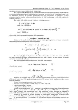
to 10.000 ft. (Fig. (1))
Because of it is used as a Flight Control Research Laboratory (FCRL) the studied aircraft is equipped
with a research avionic system composed by sensors and computers and their relative power supply subsystem.
In particular the Sensors subsystem consists of :
 Inertial Measurement Unit (three axis accelerometers and gyros)
 Magnetometer (three axis)
 Air Data Boom (static and total pressure port, vane sense for angle of attack and sideslip)
 GPS Receiver and Antenna
 Linear Potentiometers (Aileron, Elevator, Rudder and Throttle Command)
 RPM (Hall Effect Gear Tooth Sensor)
 Outside air temperature Sensor
Geometrical characteristics of the subject vehicle are:
 Wing area S: 120 ft2
 Wing chord c: 3.934 ft
 Wing span b: 30.5 ft

3. Automatic Landing System for Civil Unmanned Aerial System
www.ijeijournal.com Page | 46
Fig. 1 Flight Research Laboratory L.A.U.R.A.
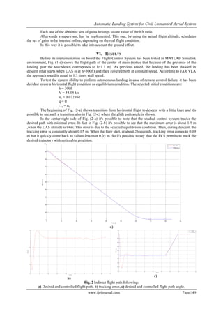
III. UAS MATHEMATICAL MODEL
When an aircraft flies close to the ground, this imposes a boundary condition which inhibits the
downward flow of air associated with the lifting action of wing and tail. The reduced downwash mainly reduces
both the downwash angle ε and the aircraft induced drag, therefore it increases both the wing-body and the tail
lift slope. Therefore, the lift increases, the neutral point shifts, the pitching moment at zero lift varies. So,
stability derivatives In Ground Effect must be used during take-off and landing for aircraft altitudes similar to
the wing span b.
Because of these effects, stability derivatives have to be modified and so it is very important a
mathematical model which afford to evaluate their behavior in ground effect.
Therefore, for ground distance h ≤ b it's necessary to evaluate the h-derivatives.
In previous researches [11], [12], a mathematical general methodology has been tuned up to evaluate
the aerodynamic characteristics variation laws due to the altitude. Such a methodology permits the calculation of
aerodynamic coefficients either OGE or IGE. It has been found that aerodynamic coefficients can be expressed
by means of hyperbolic equations [11].
According to [18], to evaluate the influence of ground effect on aerodynamic coefficients the variation
of either angle of attack (α), or downwash angle (ε) or aspect ratio (A) due to flight altitude have been modeled
by using classical methodologies [13], [19] by:
(1)
where:
 represents the vortex effect on the lift;
 A represents the aspect ratio;
 represents the cord in the wedge wing section;
 represents the lift coefficient, in this case it is the value in the equilibrium position;
 represents a correction factor that take into account of the vortex non linear effects on the lift;
 represents the non linear correction factor for taking into account that the wing is finite
(2)
where:
 Hh e Hw represent the tail and wing height from the ground;
 beff represents a non linear term that links contributes due to the wing span in IGE condition. It can be
expressed by:

4. Automatic Landing System for Civil Unmanned Aerial System
www.ijeijournal.com Page | 47
where:
 represents the lift coefficient in OGE condition;
 represents the lift increase in OGE condition;
 is calculated by and the ratio is known in literature;
 is calculated by and the ratio is in literature.
(3)
By using Eq. (1), Eq. (2) and Eq. (3) the longitudinal stability derivatives may be determined as:
(4)
IV. FLIGHT PATH MODEL
As it is known, the landing procedure is constituted of a slope segment and a flare. Obviously the glide
slope phase start out of ground effect, afterwards ground effect is to take into account. Therefore because of, as
previous stated, strong variation of aerodynamic coefficients are due to ground effect, a non linear model of the
studied aircraft should be used. To overcome this difficulty an original landing geometry has been chosen:
 The first part starts when UAS is at h=300ft and it is a constant speed descent until h=b with a glide slope
angle γ=-6° (because there are not passengers, and so it's not necessary take into account some wealth
requirement, it's possible don't consider flight path angle γ limitations);
 The second part is a constant speed flare which start when h=b (UAS in IGE condition).
Therefore it has been divided the second condition in five steps based on the values of the h/b ratio.
Each one of these steps have a 0.2 h/b ratio size. So the first step is from h/b=1 to h/b=0.8 and so on (in this way

5. Automatic Landing System for Civil Unmanned Aerial System
www.ijeijournal.com Page | 48
there are not strong variation of flight altitude in each step).
This subdivision has been necessary to employ the linearization at several equilibrium flight conditions
over the desired flight path; then the small disturbance theory may be applied. In this way difficulties due to the
use of nonlinear models of the aircraft in ground effect have been overcome and, in particular, it has been
obtained six stability matrices and six control matrices (one for OGE condition and five for IGE condition for
each kind of matrices).
The studied flight path is governed by the two following equations:
for
for
(5)
where x=0 h= 300 ft represents the beginning of the landing path.
V. AUTOMATIC LANDING SYSTEM
Because of the small disturbance theory permits to decouple longitudinal and lateral motion only
longitudinal equations have been used in the present study.
(6)
Considering Eq. (4), stability derivatives have been calculated in one value of h/b inside each of the
five steps considered. Because of altitude variation inside each step is small, it has been possible to consider
derivatives constant inside each step.
The above hypothesis bring to the following linear state space equation:
(7)
where the state vector is
(8)
and the control vector is
(9)
Air speed and flight path angle has been controlled during the whole procedure. In particular deflection
of elevator is used to control the speed while the deflections of elevator and throttle together are used to control.
the flight path angle.
Besides following requirements have been imposed:
 maximum tracking error less than 10% during the studied flight path;
 rise time smaller than 5 seconds;
 settling time smaller than 15 seconds
Because of during the landing flare it is necessary to correlate the vertical speed to the instantaneous
distance from ground, an altitude control has been effected through an external P feed forward control loop.
Such a system is engaged from flight altitude from 6 m to touch down. Elevator deflections are employed to
control flight altitude. Obviously such a system improves the precision of the controller in flight path following.
Because of, as stated in the previous paragraph, six linear models of the studied aircraft have been
obtained six multiple PID controllers have been designed by using time domain specifications.
In particular the elevator PID controllers are MISO systems, whereas the throttle PID controllers are
SISO systems.

6. Automatic Landing System for Civil Unmanned Aerial System
www.ijeijournal.com Page | 49
Each one of the obtained sets of gains belongs to one value of the h/b ratio.
Afterwards a supervisor, has be implemented. This one, by using the actual flight altitude, schedules
the set of gains to be inserted online, depending on the real flight condition.
In this way it is possible to take into account the ground effect.
VI. RESULTS
Before its implementation on board the Flight Control System has been tested in MATLAB Simulink
environment, Fig. (1-a) shows the flight path of the center of mass (notice that because of the presence of the
landing gear the touchdown corresponds to h=1.1 m). As previous stated, the landing has been divided in
descent (that starts when UAS is at h=300ft) and flare covered both at constant speed. According to JAR VLA
the approach speed is equal to 1.3 times stall speed.
To test the system ability to perform autonomous landing in case of remote control failure, it has been
decided to use a horizontal flight condition as equilibrium condition. The selected initial conditions are:
h = 300ft
V = 54.08 kts
αe = 0.072 rad
q = 0
ϑe = αe
The beginning of Fig. (2-a) shows transition from horizontal flight to descent with a little knee and it's
possible to see such a transition also in Fig. (2-c) where the glide path angle is shown.
In the center-right side of Fig. (2-a) it's possible to note that the studied control system tracks the
desired path with minimal error. In fact in Fig. (2-b) it's possible to see that the maximum error is about 1.9 m
,when the UAS altitude is 94m: This error is due to the selected equilibrium condition. Then, during descent, the
tracking error is constantly about 0.05 m. When the flare start, at about 26 seconds, tracking error comes to 0.09
m but it quickly come back to values less than 0.05 m. So it's possible to say that the FCS permits to track the
desired trajectory with noticeable precision.
a)
b)
c)
Fig. 2 Indirect flight path following:
a) Desired and controlled flight path, b) tracking error, c) desired and controlled flight path angle.

7. Automatic Landing System for Civil Unmanned Aerial System
www.ijeijournal.com Page | 50
This affirmation is comforted also with the Fig (2-c) observation, in fact it's possible to note that
desired flight path angle and real flight path angle are overlapped except for few. seconds when the descent
starts and when the flare starts.
Obviously, to design the Automatic Landing System the classical hypotheses of air at rest has been
made. To verify either robustness properties of the controller or its ability to reject disturbances several
operating situations such as flight in the presence of gust, rear or front wind and atmospheric turbulence have
been considered. Some of the most relevant results are shown in Fig. (3). It refers to a vertical gust that modifies
the aircraft angle of attack of Δα= -1 deg. The vertical gust is inserted into the model at the start of the flare
maneuver. Despite of the angle of attack reduction, due to the gust, it is interesting to note that the aircraft
performs the flare with a noticeable precision. In fact either the desired flight path or the flight path angle (Fig.
3-a) are followed with negligible errors. Figure (3-b) shows a comparison between tracking errors. It is possible
to note that the maximum error is 0.08 m. The mean value of the tracking error is 0.049 m during the whole flare
phase. Near the touch down the stabilized tracking error is about 0.02 m.
a)
b)
Fig. 3 Indirect flight path following with gust:
a) Desired and controlled flight path angle, b) tracking error comparison

8. Automatic Landing System for Civil Unmanned Aerial System
www.ijeijournal.com Page | 51
VII. CONCLUSION
The obtained results show the effectiveness of the designed Automatic Landing System. Therefore
these ones show a good accuracy of the control system for trajectory tracking in ground proximity. In fact the
UAS follows the desired flight path with a noticeable precision. The following original contributions can be
highlight: 1) the obtained model of the aerodynamic coefficient In Ground Effect that afford to evaluate stability
and control derivatives variations during the landing 2) the use of airspeed and glide path angle as controlled
variables during the whole landing 3) the landing geometry.
Further developments of the present research will be the extension of the designed control system to
the take-off phase.
Afterwards the aircraft model will be improved by evaluating both lateral stability derivatives
variations In Ground Effect and the bank angle derivatives (φ derivatives). Since the present methodology will
be employed to design a Lateral Automatic Landing System.
At the present flight tests are performing to verify the effectiveness of the designed Automatic
Longitudinal Landing System by means of the above described Flight Control Research Laboratory. The
obtained results could be used later on, with the purpose to realize a fully autonomous UAS.
ACKNOWLEDGEMENTS
This paper has been realized with the financial support of the Italian University and Scientific Research
Minister in the context of the PRIN 2008.
REFERENCES
[1] Schawe, D.; Rohardt, C. H.; Wichmann, G.; Aerodynamic design assessment of Strato 2C and its potential for unmanned high
altitude airborne platforms, Aerospace Science and Technology Vol .6,2002, pp.43-51
[2] Nelson, R.C.; Flight Stability and Automatic Control, McGraw-Hill Book Company, NewYork, 1989
[3] Stevens, B.L.; Lewis, F. L.; Aircraft Control and Simulation, John Wiley & Sons,Inc., New York, 1992
[4] Blakelock, J. H.; Automatic control of Aircraft & Missiles, John Wiley & Sons, Inc., New York, 1992
[5] Ohno, M.; Yasuhiro, Y.; Hata, T.; Takahama, M.; Miyazawa, Y.; Izumi, T.; Robust flight control law design for an automatic
landing flight experiment, Control Engineering Practice , Vol 7, 1999, pp. 1143-1151
[6] Che, J.; Chen, D.; Automatic landing control using H-inf control and stable inversion, Proceedings of The 40th
Conference on
Decision and Control, 2001, pp.241-246
[7] Pashilkar, A. A.; Sundadadajan N.;Saratchhandran P.A.; Fault-tolerant neural aided controller for aircraft auto-landing, Aerospace
Science and Technology, Vol. 10 N.1,2006, p.p. 49-61
[8] Rong, H. J. et al.; Adaptive fuzzy fault-tolerant control for aircraft autolanding under failure, IEEE Transactions on Aerospace and
Electronic Systems Vol. 43 No. 4, 2007, pp.1586-1603
[9] Lungu ,L.; Lungu, M.; Grigorie, L. T.; Automatic Control of Aircraft in Longitudinal Plane During Landing, IEEE Transactions on
Aerospace and Electronic Systems Vol. 49 No. 2,2013, pp.1338-1350
[10] Riseborough, P.; Automatic Take-off and Landing Control for Small UAV’s, Proceedings of The 5th
Asian Control Conference,
2004,Vol 2,pp.754-762
[11] Grillo, C.; Gatto, C.; Dynamic Stability of Wing in Ground Effect Vehicles: a General Model, Proceedings of The 8th
International
Conference on Fast Sea Transportation,2005(on CD-ROM)
[12] Grillo, C.; Gatto, C.; Caccamo, C.; Pizzolo, A.; A Non Conventional UAV In Ground Effect: Synthesis of a Robust Flight
Control System, Automatic Control in Aerospace Vol. 2,2008, p.p.1-8
[13] Roskam, J.; Airplane Design , part VI , Preliminary calculation of Aerodynamic, Thrust and Power Characteristics, The University
of Kansas, 1990
[14] Curry, R. E.; Moulton, B. J.; Kresse, J.; An in-flight investigation of ground effect on a forward-swept wing airplane, NASA T.N.
101708, 1989.
[15] Amato, F.; Mattei, M.; Scala, S.; Verde, L.; Robust flight control design for the HIRM based on Linear Quadratic Control,
Aerospace Sciences & Technologies, Vol. 4, 2000, pp.423-438
[16] Hata, T.; Onuma, H.; Miyazawa, Y.; Izumi, T.; Flight control system for ALFLEX, Proceedings of The second Asian Control
Conference, Seoul, 2004, Vol. 2,pp.31-34
[17] Kovacic, Z.; Bogdan, S.; Fuzzy Controller Design- Theory and Applications, Taylor and Francis,2006
[18] Rozhdestvensky, K. V; Aerodynamics of a lifting system in extreme ground effect, Springer,2000
[19] AA.VV.; Engineering Data ESDU, IHS, 1972