Design and state space modelling of a TCV Rocket using Simulink and Matlab with Gimbal Angle, Angular Velocity and Drift experienced as our control parameters. - Using LQR control to stabilize the model. - Support why LQR is used over PID control for TCV Modelling.

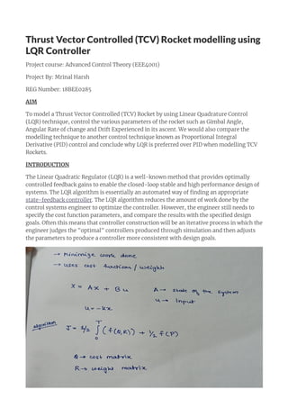
1. Thrust Vector Controlled (TCV) Rocket modelling using
LQR Controller
Project course: Advanced Control Theory (EEE4001)
Project By: Mrinal Harsh
REG Number: 18BEE0285
AIM
To model a Thrust Vector Controlled (TCV) Rocket by using Linear Quadrature Control
(LQR) technique, control the various parameters of the rocket such as Gimbal Angle,
Angular Rate of change and Drift Experienced in its ascent. We would also compare the
modelling technique to another control technique known as Proportional Integral
Derivative (PID) control and conclude why LQR is preferred over PID when modelling TCV
Rockets.
INTRODUCTION
The Linear Quadratic Regulator (LQR) is a well-known method that provides optimally
controlled feedback gains to enable the closed-loop stable and high performance design of
systems. The LQR algorithm is essentially an automated way of finding an appropriate
state-feedback controller. The LQR algorithm reduces the amount of work done by the
control systems engineer to optimize the controller. However, the engineer still needs to
specify the cost function parameters, and compare the results with the specified design
goals. Often this means that controller construction will be an iterative process in which the
engineer judges the "optimal" controllers produced through simulation and then adjusts
the parameters to produce a controller more consistent with design goals.

2. DESIGN PROBLEM AND EQUATIONS
Controlling the flight of the rocket during the launch phase as it’s the state most prone to
failure due to disturbances and has to clear the atmosphere safely.
Input to be controlled: Gimbal Angle (The angle between the thrust and the perpendicular)
Outputs: Pitch Angle ( theta), Angular Velocity (theta dot) and Drift experienced by the
TCV (Z)
DRIFT- A phenomenon that occurs in vehicles that use ascent and is caused due to the
wind. It makes the vehicle move sideways, causing unpredictability in our flight.

4. MATLAB CODE:
%%% STATE SPACE MODELLING %%%
clc;
close all;
clear all;
%cosntant values
Iyy=2.186e8; %[Slug ft^2]
m=38901; %[Slug]
Tc=2.361e6; %[lbf]
V=1347; %[ft/s]
Cn_alpha=0.1465;
g=26.10; %[ft/s^2]
N_alpha=686819; %[lbf/rad]
M_alpha=0.3807; %[s^-2]
M_delta=0.5726; %[s^-2]
x_cg=53.19; %[ft]
x_cp=121.2; %[ft]
F=Tc;
%Other important constants
Mach=1.4 %mach
h=34000; %height of the launch vehicle
S=116.2; %Area of the platform
Fbase=1000; %base drag
Ca=2.4; %coefficients
D=Ca*680*S - Fbase; %drag
Drag=7.15*D %total drag
%state space matrix
A_m=[0 1 0;M_alpha 0 M_alpha/V;-(F-Drag+N_alpha)/m 0 -N_alpha/(m*V)];
B_m=[0;M_delta;Tc/m];
C_m=diag([1 1 1]);
D_m=[0;0;0];
pitch_ss=ss(A_m,B_m,C_m,D_m);
%%% COST FUNCTION %%%
%cost function

5. SIMULINK MODELS:
Main TCV Model
Subsystem Model
cvector={'bo' 'ro' 'go'};
R_vector=[0.1 5 10]
%lowest weight to TVC angle, max to drift
figure;hold on;
for k=1:1
R_matrix_drift=R_vector(k);
Q_matrix_drift=[1 0 1/V; 0 0 0;1/V 0 1/V^2];
[K S e]=lqr(pitch_ss,Q_matrix_drift,R_matrix_drift);
for i=1:10000
e_val(:,i)=eig(A_m-B_m*K*i/10000);
end
plot(real(e_val(1,:)),imag(e_val(1,:)),cvector{k});
plot(real(e_val(2,:)),imag(e_val(2,:)),cvector{k});
plot(real(e_val(3,:)),imag(e_val(3,:)),cvector{k});
grid;
end
xlim([-2 1]);
legend('R=0.1');
%LQR Gains are obtained
K_1=K(1);
K_2=K(2);
K_3=K(3);

6. RESULTS
Controllability and Stability of the System
For analysing a system using LQE we need to make sure that the system is
controllable and observable. Since the rank of A_m matrix is same as the rank of Qc
(controllability matrix) and Qb (stability matrix), the obtained state space model is
controllable and stable.
Root Locus of the System

7. To check stability of the system we plot the eigen values as root locus. As we can see,
the system is marginally stable since some values of the Root Locus graph lie on the
positive plane.
Take OFF Angle
The TVC input causes the take-off angle to increase initially but its stabilized once the
rocket starts its upward ascent.

8. Angular Rate
For a successful launch, we need the angular rate to be zero In order to cut down on
the angular spin faced by the vehicle. As seen in the plot, the Angular rate increases
initially and then decreases rapidly as the system is stabilized in mid-flight.
Drift experienced by the Rocket

9. Since we have accounted for wind speed and other physical factors in our state space
modelling equations, the system experiences a drift and a motion caused by it that
like other parameters are quite large at start but are stabilized successfully mid-
flight.
Comparisons with PID Control
As we can see in the graph alongside, PID controller used for a similar simulation
would give us faster stabilizing rate but the overshoot is greater. This gives an insight
as to why PID control can be used for small launch system but for larger, real life
system LQR control is used as a slightly greater time taken to stabilize Is compensated
by the lower overshoot which makes the system safer, especially during the initial
ascent.
Conclusion:

10. The given state space model was checked for stability and controllability and the outcome
was that it satisfied the given conditions. It was judged marginally stable by the help of its
root locus plot. The system design was successful as we could control and stabilize our
three control parameters ie. Take off angle, angular rate and drift faced by the rocket. We
compared the two most common control techniques for- Linear Quadratic Control (LQC)
and Proportional Integral & Derivative control (PID) and saw why the latter is used in real
life simulations.