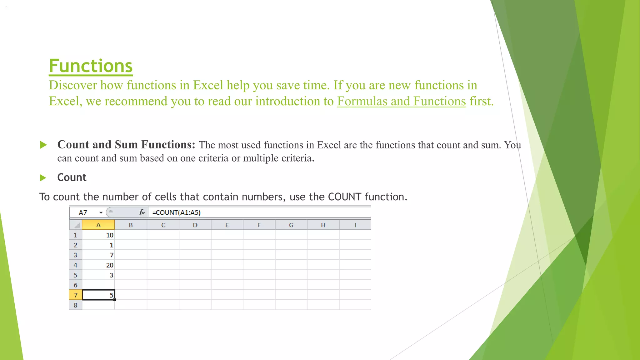
SlideShare a Scribd company logo
Excel- The Powerful Skills
Function Training
By Kapileshwar Kumar
Functions
Discover how functions in Excel help you save time. If you are new functions in
Excel, we recommend you to read our introduction to Formulas and Functions first.
 Count and Sum Functions: The most used functions in Excel are the functions that count and sum. You
can count and sum based on one criteria or multiple criteria.
 Count
To count the number of cells that contain numbers, use the COUNT function.
.
 Countif
To count cells based on one criteria (for example, higher than 9), use the following COUNTIF function.
Countifs
 To count cells based on multiple criteria (for example, green and higher than 9), use the
following COUNTIFS function.
 Sum
To sum a range of cells, use the SUM function.
 Sumif
To sum cells based on one criteria (for example, higher than 9), use the following SUMIF function (two
arguments).
To sum cells based on one criteria (for example, green), use the following SUMIF function (three
arguments, last argument is the range to sum).
 Sumifs
To sum cells based on multiple criteria (for example, blue and green), use the following SUMIFS
function (first argument is the range to sum).
General note: in a similar way, you can use the AVERAGEIF and AVERAGEIFS function to average
cells based on one or multiple criteria.
Logical Functions:
Learn how to use Excel's logical functions such as the IF, AND and OR function.
 If Function
The IF function checks whether a condition is met, and returns one value if TRUE and another
value if FALSE.
1. Select cell C2 and enter the following function.
The IF function returns Correct because the value in cell A1 is higher than 10.
 And Function
The AND Function returns TRUE if all conditions are true and returns FALSE if any of the
conditions are false.
1. Select cell D2 and enter the following formula.
The AND function returns FALSE because the value in cell B2 is not higher than 5. As a result the IF
function returns Incorrect.
 Or Function
The OR function returns TRUE if any of the conditions are TRUE and returns FALSE if all
conditions are false.
1. Select cell E2 and enter the following formula.
The OR function returns TRUE because the value in cell A1 is higher than 10. As a result the IF
function returns Correct.
General note: the AND and OR function can check up to 255 conditions.
Date & Time Functions
To enter a date in Excel, use the "/" or "-" characters. To enter a time, use the ":" (colon). You can also
enter a date and a time in one cell.
Note: Dates are in US Format. Months first, Days second. This type of format depends on your
windows regional settings. Learn more about Date and Time formats
In the Category list, select Date, and select a Date format
 Year, Month, Day
To get the year of a date, use the YEAR function
Note: use the MONTH and DAY function to get the month and day of a
date.
 Date Function
1. To add a number of days to a date, use the following simple formula.
2. To add a number of years, months and/or days, use the DATE function.
Note: the DATE function accepts three arguments: year, month and day. Excel knows that 6 + 2 = 8 =
August has 31 days and rolls over to the next month (23 August + 9 days = 1 September).
 Current Date & Time
To get the current date and time, use the NOW function.
Note: use the TODAY function to get the current date only. Use NOW()-TODAY() to get the current
time only (and apply a Time format).
 Hour, Min, Sec
To return the hour, use the HOUR function.
Note: use the MINUTE and SECOND function to return the minute and
second.
 Time Function
To add a number of hours, minutes and/or seconds, use the TIME function.
Note: Excel adds 2 hours, 10 + 1 = 11 minutes and 70 - 60 = 10
seconds.
Text Functions
Excel has many functions to offer when it comes to manipulating text strings.
Join Strings
To join strings, use the & operator
Note: to insert a space, use " "
 Left
To extract the leftmost characters from a string, use the LEFT function.
 Right
To extract the rightmost characters from a string, use the RIGHT function.
 Mid
To extract a substring, starting in the middle of a string, use the MID function.
Note: started at position 5 (p) with length 3.
 Len
To get the length of a string, use the LEN function.
Note: space (position 8) included!
 Find
To find the position of a substring in a string, use the FIND function.
Note: string "am" found at position 3.
 Substitute
To replace existing text with new text in a string, use the SUBSTITUTE function.
Lookup & Reference Functions
Learn all about Excel's lookup & reference functions such as the VLOOKUP,
HLOOKUP, MATCH, INDEX and CHOOSE function.
 VLookup
The VLOOKUP (Vertical lookup) function looks for a value in the leftmost column of a table, and then
returns a value in the same row from another column you specify.
1. Insert the VLOOKUP function shown below.
Explanation: the VLOOKUP function looks for the ID (104) in the leftmost column of the range
$E$4:$G$7 and returns the value in the same row from the third column (third argument is set to 3). The
fourth argument is set to FALSE to return an exact match or a #N/A error if not found.
2. Drag the VLOOKUP function in cell B2 down to cell B11.
Note: when we drag the VLOOKUP function down, the absolute reference ($E$4:$G$7) stays the same, while the
relative reference (A2) changes to A3, A4, A5, etc.
 HLookup
In a similar way, you can use the HLOOKUP (Horizontal lookup)
function.
 Match
The MATCH function returns the position of a value in a given range.
Note: Yellow found at position 3 in the range E4:E7. The third argument is optional. Set this argument to 0 to
return the position of the value that is exactly equal to lookup value (A2) or a #N/A error if not found.
 Index
The INDEX function returns a specific value in a two-dimensional or
one-dimensional range.
Note: 92 found at the intersection of row 3 and column 2 in the range E4:F7.
Note: 97 found at position 3 in the range E4:E7.
 Choose
The CHOOSE function returns a value from a list of values, based on a
position number
Note: Boat found at position 3.
Financial Functions
To illustrate Excel's most popular financial functions, we consider a loan with monthly payments, an
annual interest rate of 6%, a 20-year duration, a present value of $150,000 (amount borrowed) and a future
value of 0 (that's what you hope to achieve when you pay off a loan).
We make monthly payments, so we use 6%/12 = 0.5% for Rate and 20*12 = 240 for Nper (total number of
periods). If we make annual payments on the same loan, we use 6% for Rate and 20 for Nper.
 Pmt
Select cell A2 and insert the PMT function.
Note: The last two arguments are optional. For loans the Fv can be omitted (the future value of a loan equals 0,
however, it's included here for clarification). If Type is omitted, it is assumed that payments are due at the end
of the period.
Result. The monthly payment equals $1,074.65.
 Rate
If Rate is the only unknown variable, we can use the RATE function to calculate the interest rate.
 Nper
Or the NPER function. If we make monthly payments of $1,074.65 on a 20-year loan, with an annual
interest rate of 6%, it takes 240 months to pay off this loan.
We already knew this, but we can change the monthly payment now to see how this affects the total
number of periods.
Conclusion: if we make monthly payments of $2,074.65, it takes less than 90 months to pay off this loan.
 Pv
Or the PV (Present Value) function. If we make monthly payments of $1,074.65 on a 20-year loan, with an annual
interest rate of 6%, how much can we borrow? You already know the answer.
 Fv
And we finish this chapter with the FV (Future Value) function. If we make monthly payments of
$1,074.65 on a 20-year loan, with an annual interest rate of 6%, do we pay off this loan? Yes.
But, if we make monthly payments of only $1,000.00, we still have debt after 20 years.
Statistical Functions
This chapter gives an overview of some very useful statistical functions in Excel.
 Average
To calculate the average of a range of cells, use the AVERAGE
function.
 Averageif
To average cells based on one criteria, use the AVERAGEIF function. For example, to calculate the average
excluding zeros.
Note: <> means not equal to. The AVERAGEIF function is similar to
the SUMIF function.
 Median
To find the median (or middle number), use the MEDIAN function.
Check:
 Mode
To find the most frequently occurring number, use the MODE function.
 Standard Deviation
To calculate the standard deviation, use the STEDV function.
 Min
To find the minimum value, use the MIN function
 Max
To find the maximum value, use the MAX function
 Large
To find the third largest number, use the following LARGE function.
Check:
 Small
To find the second smallest number, use the following SMALL function.
Check:
Tip: Excel can generate most of these results with the click of a button.
Our Descriptive Statistics example shows you how.
Round
This chapter illustrates three functions to round numbers in Excel. The ROUND, ROUNDUP and
ROUNDDOWN function.
Before your start: if you round a number, you lose precision. If you don't want this, show fewer
decimal places without changing the number itself.
 Round
 1. Round a number to two decimal places.
Note: 1, 2, 3, and 4 get rounded down. 5, 6, 7, 8, and 9 get rounded up. In this example, 114.7211, 114.7221,
114.7231 and 114.7241 get rounded down to 114.72 and 114.7251, 114.7261, 114.7271, 114.7281 and 114.7291
get rounded up to 114.73.
2. Round a number to one decimal place.
3. Round a number to the nearest integer.
4. Round a number to the nearest 10.
5. Round a number to the nearest 100.
 RoundUp
The ROUNDUP function always rounds a number up (away from zero). For example, round a number up
to one decimal place.
 RoundDown
The ROUNDDOWN function always rounds a number down (toward zero). For example, round a number down to
the nearest integer.
Formula Errors
This chapter teaches you how to deal with some common formula errors in Excel.
 ##### error
When your cell contains this error code, the column isn't wide enough to display the value.
1. Click on the right border of the column A header and increase the column width.
Tip: double click the right border of the column A header to automatically fit the widest cell in column A.
 #NAME? error
The #NAME? error occurs when Excel does not recognize text in a formula.
1. Simply correct SU to SUM.
 #VALUE! error
Excel displays the #VALUE! error when a formula has the wrong type of argument.
1a. Change the value of cell A3 to a number.
1b. Use a function to ignore cells that contain text.
 #DIV/0! error
Excel displays the #DIV/0! error when a formula tries to divide a number by 0 or an empty cell.
1a. Change the value of cell A2 to a value that is not equal to 0.
1b. Prevent the error from being displayed by using the logical function IF.
Explanation: if cell A2 equals 0, an empty string is displayed. If not, the result of the formula A1/A2 is
displayed.
 #REF! error
Excel displays the #REF! error when a formula refers to a cell that is not valid.
1. Cell C1 references cell A1 and cell B1.
2. Delete column B. To achieve this, right click the column B header and click Delete.
3. Select cell B1. The reference to cell B1 is not valid anymore.
4. To fix this error, you can either delete +#REF! in the formula of cell B1 or you can undo your action by
clicking Undo in the Quick Access Toolbar (or press CTRL + z).
Array Formulas
This chapter helps you understand array formulas in Excel. Single cell array formulas perform
multiple calculations in one cell.
 Without Array Formula
Without using an array formula, we would execute the following steps to find the greatest progress.
1. First, we would calculate the progress of each student.
2. Next, we would use the MAX function to find the greatest progress.
 With Array Formula
We don't need to store the range in column D. Excel can store this range in its memory. A range stored in
Excel's memory is called an array constant.
1. We already know that we can find the progress of the first student by using the formula below.
2. To find the greatest progress (don't be overwhelmed), we add the MAX function, replace C2 with C2:C6 and B2
with B2:B6.
3. Finish by pressing CTRL + SHIFT + ENTER.
Note: The formula bar indicates that this is an array formula by enclosing it in curly braces {}. Do not type these
yourself. They will disappear when you edit the formula.
Explanation: The range (array constant) is stored in Excel's memory, not in an range. The array constant looks as
follows:
{19;33;63;48;13}
This array constant is used as an argument for the MAX function, giving a result of 63.
 F9 Key
When working with array formulas, you can have a look at these array constants yourself.
1. Select C2:C6-B2:B6 in the formula.
2. Press F9.
That looks good. Elements in a vertical array constant are separated by semicolons. Elements in a horizontal
array constant are separated by commas.
Excel Function Training

More Related Content

What's hot

Excel lesson formulas and functions
Excel lesson formulas and functionsExcel lesson formulas and functions
Excel lesson formulas and functionswildman099
 
Excel IF function
Excel IF functionExcel IF function
Excel IF functionHtay Aung
 
Excel Tutorials - VLOOKUP and HLOOKUP Functions
Excel Tutorials - VLOOKUP and HLOOKUP FunctionsExcel Tutorials - VLOOKUP and HLOOKUP Functions
Excel Tutorials - VLOOKUP and HLOOKUP Functions
Merve Nur Taş
 
Ppt on pivot table
Ppt on pivot tablePpt on pivot table
Ppt on pivot table
Hemendra Vyas
 
10 Excel Formulas that will help you in any Job
10 Excel Formulas that will help you in any Job10 Excel Formulas that will help you in any Job
10 Excel Formulas that will help you in any Job
Hitesh Biyani
 
How to use Hlookup find an exact match
How to use Hlookup find an exact match How to use Hlookup find an exact match
How to use Hlookup find an exact match
Excel Advise
 
Ms excel
Ms excelMs excel
3. lookup functions in excel
3. lookup functions in excel3. lookup functions in excel
3. lookup functions in excel
Dr. Prashant Vats
 
Vlookup - an introduction
Vlookup - an introductionVlookup - an introduction
Vlookup - an introduction
vvmenon22
 
Using vlookup in excel
Using vlookup in excelUsing vlookup in excel
Using vlookup in excelmegankilb
 
03.names and ranges
03.names and ranges03.names and ranges
03.names and ranges
Steven Alphonce
 
Formula in MS Excel
Formula in MS ExcelFormula in MS Excel
Formula in MS Excel
Muhammad Yasir Bhutta
 
Basic Ms excel
Basic Ms excelBasic Ms excel
Basic Ms excel
maharzahid0
 
Microsoft Excel 101
Microsoft Excel 101Microsoft Excel 101
Microsoft Excel 101
Louis Honeyman
 
Ms excel
Ms excelMs excel
Ms excel
HebaKidwai2
 
05.formatting cells
05.formatting cells05.formatting cells
05.formatting cells
Steven Alphonce
 
Excel lesson01
Excel lesson01Excel lesson01
Excel lesson01
Erik Hardiyanto
 
VLOOKUP Function - Marelen Talavera - Vivacious Analytic
VLOOKUP Function - Marelen Talavera - Vivacious AnalyticVLOOKUP Function - Marelen Talavera - Vivacious Analytic
VLOOKUP Function - Marelen Talavera - Vivacious Analytic
Maria Elena Acdol-Talavera
 
Excel CountIf with Multiple Criteria
Excel CountIf with Multiple CriteriaExcel CountIf with Multiple Criteria
Excel CountIf with Multiple Criteria
Chester Tugwell
 

What's hot (20)

Excel lesson formulas and functions
Excel lesson formulas and functionsExcel lesson formulas and functions
Excel lesson formulas and functions
 
Excel IF function
Excel IF functionExcel IF function
Excel IF function
 
Excel Tutorials - VLOOKUP and HLOOKUP Functions
Excel Tutorials - VLOOKUP and HLOOKUP FunctionsExcel Tutorials - VLOOKUP and HLOOKUP Functions
Excel Tutorials - VLOOKUP and HLOOKUP Functions
 
Ppt on pivot table
Ppt on pivot tablePpt on pivot table
Ppt on pivot table
 
10 Excel Formulas that will help you in any Job
10 Excel Formulas that will help you in any Job10 Excel Formulas that will help you in any Job
10 Excel Formulas that will help you in any Job
 
How to use Hlookup find an exact match
How to use Hlookup find an exact match How to use Hlookup find an exact match
How to use Hlookup find an exact match
 
Ms excel
Ms excelMs excel
Ms excel
 
3. lookup functions in excel
3. lookup functions in excel3. lookup functions in excel
3. lookup functions in excel
 
Vlookup - an introduction
Vlookup - an introductionVlookup - an introduction
Vlookup - an introduction
 
Using vlookup in excel
Using vlookup in excelUsing vlookup in excel
Using vlookup in excel
 
03.names and ranges
03.names and ranges03.names and ranges
03.names and ranges
 
Formula in MS Excel
Formula in MS ExcelFormula in MS Excel
Formula in MS Excel
 
Introduction to microsoft excel 2007
Introduction to microsoft excel 2007Introduction to microsoft excel 2007
Introduction to microsoft excel 2007
 
Basic Ms excel
Basic Ms excelBasic Ms excel
Basic Ms excel
 
Microsoft Excel 101
Microsoft Excel 101Microsoft Excel 101
Microsoft Excel 101
 
Ms excel
Ms excelMs excel
Ms excel
 
05.formatting cells
05.formatting cells05.formatting cells
05.formatting cells
 
Excel lesson01
Excel lesson01Excel lesson01
Excel lesson01
 
VLOOKUP Function - Marelen Talavera - Vivacious Analytic
VLOOKUP Function - Marelen Talavera - Vivacious AnalyticVLOOKUP Function - Marelen Talavera - Vivacious Analytic
VLOOKUP Function - Marelen Talavera - Vivacious Analytic
 
Excel CountIf with Multiple Criteria
Excel CountIf with Multiple CriteriaExcel CountIf with Multiple Criteria
Excel CountIf with Multiple Criteria
 

Similar to Excel Function Training

Ms excel commands
Ms excel commandsMs excel commands
Ms excel commands
DiyaVerma14
 
The 4 Step Excel 2013 Functions Guide
The 4 Step Excel 2013 Functions GuideThe 4 Step Excel 2013 Functions Guide
The 4 Step Excel 2013 Functions Guide
How To Technology
 
Lesson9 Working With Basic Functions
Lesson9 Working With Basic FunctionsLesson9 Working With Basic Functions
Lesson9 Working With Basic Functionsguevarra_2000
 
Excel Useful Tips
Excel Useful TipsExcel Useful Tips
Excel Useful TipsParul_100in
 
E-Book 25 Tips and Tricks MS Excel Functions & Formulaes
E-Book 25 Tips and Tricks MS Excel Functions & FormulaesE-Book 25 Tips and Tricks MS Excel Functions & Formulaes
E-Book 25 Tips and Tricks MS Excel Functions & Formulaes
BurCom Consulting Ltd.
 
Basic Functions - Excel 2013 Tutorial
Basic Functions - Excel 2013 TutorialBasic Functions - Excel 2013 Tutorial
Basic Functions - Excel 2013 Tutorial
SpreadsheetTrainer
 
Lesson9 working with basic functions
Lesson9 working with basic functionsLesson9 working with basic functions
Lesson9 working with basic functionsricsanmae
 
In Section 1 on the Data page, complete each column of the spreads.docx
In Section 1 on the Data page, complete each column of the spreads.docxIn Section 1 on the Data page, complete each column of the spreads.docx
In Section 1 on the Data page, complete each column of the spreads.docx
sleeperharwell
 
Advanced Spreadsheet Skills-1.pptx
Advanced Spreadsheet Skills-1.pptxAdvanced Spreadsheet Skills-1.pptx
Advanced Spreadsheet Skills-1.pptx
CliffordBorromeo
 
Functions and formulas of ms excel
Functions and formulas of ms excelFunctions and formulas of ms excel
Functions and formulas of ms excel
madhuparna bhowmik
 
Use of Excel Spreadsheets in Computing Grades
Use of Excel Spreadsheets in Computing GradesUse of Excel Spreadsheets in Computing Grades
Use of Excel Spreadsheets in Computing Grades
Elli May Cañas
 
functionsandformulas-131221213835-phpapp01.pdf
functionsandformulas-131221213835-phpapp01.pdffunctionsandformulas-131221213835-phpapp01.pdf
functionsandformulas-131221213835-phpapp01.pdf
FranzLawrenzDeTorres1
 
50 MS Excel Tips and Tricks
50 MS Excel Tips and Tricks 50 MS Excel Tips and Tricks
50 MS Excel Tips and Tricks
BurCom Consulting Ltd.
 
Microsoft Excel 20072010 What-If Analysis © Martin Green
Microsoft Excel 20072010  What-If Analysis © Martin GreenMicrosoft Excel 20072010  What-If Analysis © Martin Green
Microsoft Excel 20072010 What-If Analysis © Martin Green
DioneWang844
 
computer applications in business unit 3
computer applications in business unit 3computer applications in business unit 3
computer applications in business unit 3
Dr T.Sivakami
 
Excel.fns frmls
Excel.fns frmlsExcel.fns frmls
Excel.fns frmls
rowenick
 
2. mathematical functions in excel
2. mathematical functions in excel2. mathematical functions in excel
2. mathematical functions in excel
Dr. Prashant Vats
 
Excel11
Excel11Excel11
Excel11
acharyaa
 
Top 20 microsoft excel formulas you must know
Top 20 microsoft excel formulas you must knowTop 20 microsoft excel formulas you must know
Top 20 microsoft excel formulas you must know
AlexHenderson59
 

Similar to Excel Function Training (20)

Ms excel commands
Ms excel commandsMs excel commands
Ms excel commands
 
The 4 Step Excel 2013 Functions Guide
The 4 Step Excel 2013 Functions GuideThe 4 Step Excel 2013 Functions Guide
The 4 Step Excel 2013 Functions Guide
 
Lesson9 Working With Basic Functions
Lesson9 Working With Basic FunctionsLesson9 Working With Basic Functions
Lesson9 Working With Basic Functions
 
Excel Useful Tips
Excel Useful TipsExcel Useful Tips
Excel Useful Tips
 
E-Book 25 Tips and Tricks MS Excel Functions & Formulaes
E-Book 25 Tips and Tricks MS Excel Functions & FormulaesE-Book 25 Tips and Tricks MS Excel Functions & Formulaes
E-Book 25 Tips and Tricks MS Excel Functions & Formulaes
 
Basic Functions - Excel 2013 Tutorial
Basic Functions - Excel 2013 TutorialBasic Functions - Excel 2013 Tutorial
Basic Functions - Excel 2013 Tutorial
 
Lesson9 working with basic functions
Lesson9 working with basic functionsLesson9 working with basic functions
Lesson9 working with basic functions
 
In Section 1 on the Data page, complete each column of the spreads.docx
In Section 1 on the Data page, complete each column of the spreads.docxIn Section 1 on the Data page, complete each column of the spreads.docx
In Section 1 on the Data page, complete each column of the spreads.docx
 
Advanced Spreadsheet Skills-1.pptx
Advanced Spreadsheet Skills-1.pptxAdvanced Spreadsheet Skills-1.pptx
Advanced Spreadsheet Skills-1.pptx
 
Functions and formulas of ms excel
Functions and formulas of ms excelFunctions and formulas of ms excel
Functions and formulas of ms excel
 
Use of Excel Spreadsheets in Computing Grades
Use of Excel Spreadsheets in Computing GradesUse of Excel Spreadsheets in Computing Grades
Use of Excel Spreadsheets in Computing Grades
 
functionsandformulas-131221213835-phpapp01.pdf
functionsandformulas-131221213835-phpapp01.pdffunctionsandformulas-131221213835-phpapp01.pdf
functionsandformulas-131221213835-phpapp01.pdf
 
50 MS Excel Tips and Tricks
50 MS Excel Tips and Tricks 50 MS Excel Tips and Tricks
50 MS Excel Tips and Tricks
 
Microsoft Excel 20072010 What-If Analysis © Martin Green
Microsoft Excel 20072010  What-If Analysis © Martin GreenMicrosoft Excel 20072010  What-If Analysis © Martin Green
Microsoft Excel 20072010 What-If Analysis © Martin Green
 
computer applications in business unit 3
computer applications in business unit 3computer applications in business unit 3
computer applications in business unit 3
 
Excel.fns frmls
Excel.fns frmlsExcel.fns frmls
Excel.fns frmls
 
2. mathematical functions in excel
2. mathematical functions in excel2. mathematical functions in excel
2. mathematical functions in excel
 
Excel11
Excel11Excel11
Excel11
 
Top 20 microsoft excel formulas you must know
Top 20 microsoft excel formulas you must knowTop 20 microsoft excel formulas you must know
Top 20 microsoft excel formulas you must know
 
Excelformulas
ExcelformulasExcelformulas
Excelformulas
 

More from kapileshwar kumar

Did you know
Did you knowDid you know
Did you know
kapileshwar kumar
 
Happy diwali
Happy diwaliHappy diwali
Happy diwali
kapileshwar kumar
 
The story of India
The story of India The story of India
The story of India
kapileshwar kumar
 
Coming soon!!! modi raz
Coming soon!!! modi razComing soon!!! modi raz
Coming soon!!! modi raz
kapileshwar kumar
 
Infosys mysore campus visit with friends
Infosys mysore campus visit with friendsInfosys mysore campus visit with friends
Infosys mysore campus visit with friendskapileshwar kumar
 
Keyword Research and Analysis
Keyword Research and AnalysisKeyword Research and Analysis
Keyword Research and Analysis
kapileshwar kumar
 
Tata first dot powered by NEN 2012
Tata first dot powered by NEN 2012Tata first dot powered by NEN 2012
Tata first dot powered by NEN 2012kapileshwar kumar
 
Think good thoughts by kapileshwar
Think good thoughts by kapileshwarThink good thoughts by kapileshwar
Think good thoughts by kapileshwar
kapileshwar kumar
 
This is my india by kapileshwar
This is my india by kapileshwarThis is my india by kapileshwar
This is my india by kapileshwarkapileshwar kumar
 
Team building by kapileshwar kumar
Team building by kapileshwar kumarTeam building by kapileshwar kumar
Team building by kapileshwar kumar
kapileshwar kumar
 

More from kapileshwar kumar (14)

Did you know
Did you knowDid you know
Did you know
 
Happy diwali
Happy diwaliHappy diwali
Happy diwali
 
Incredible india
Incredible indiaIncredible india
Incredible india
 
The story of India
The story of India The story of India
The story of India
 
Coming soon!!! modi raz
Coming soon!!! modi razComing soon!!! modi raz
Coming soon!!! modi raz
 
Smoking
SmokingSmoking
Smoking
 
Infosys mysore campus visit with friends
Infosys mysore campus visit with friendsInfosys mysore campus visit with friends
Infosys mysore campus visit with friends
 
Keyword Research and Analysis
Keyword Research and AnalysisKeyword Research and Analysis
Keyword Research and Analysis
 
Tata first dot powered by NEN 2012
Tata first dot powered by NEN 2012Tata first dot powered by NEN 2012
Tata first dot powered by NEN 2012
 
E- week india 2011 award
E- week india 2011 awardE- week india 2011 award
E- week india 2011 award
 
Think good thoughts by kapileshwar
Think good thoughts by kapileshwarThink good thoughts by kapileshwar
Think good thoughts by kapileshwar
 
This is my india by kapileshwar
This is my india by kapileshwarThis is my india by kapileshwar
This is my india by kapileshwar
 
The Beauty of Math
The Beauty of MathThe Beauty of Math
The Beauty of Math
 
Team building by kapileshwar kumar
Team building by kapileshwar kumarTeam building by kapileshwar kumar
Team building by kapileshwar kumar
 

Excel Function Training

  • 1. Excel- The Powerful Skills Function Training By Kapileshwar Kumar
  • 2. Functions Discover how functions in Excel help you save time. If you are new functions in Excel, we recommend you to read our introduction to Formulas and Functions first.  Count and Sum Functions: The most used functions in Excel are the functions that count and sum. You can count and sum based on one criteria or multiple criteria.  Count To count the number of cells that contain numbers, use the COUNT function. .
  • 3.  Countif To count cells based on one criteria (for example, higher than 9), use the following COUNTIF function. Countifs  To count cells based on multiple criteria (for example, green and higher than 9), use the following COUNTIFS function.
  • 4.  Sum To sum a range of cells, use the SUM function.  Sumif To sum cells based on one criteria (for example, higher than 9), use the following SUMIF function (two arguments). To sum cells based on one criteria (for example, green), use the following SUMIF function (three arguments, last argument is the range to sum).
  • 5.  Sumifs To sum cells based on multiple criteria (for example, blue and green), use the following SUMIFS function (first argument is the range to sum). General note: in a similar way, you can use the AVERAGEIF and AVERAGEIFS function to average cells based on one or multiple criteria.
  • 6. Logical Functions: Learn how to use Excel's logical functions such as the IF, AND and OR function.  If Function The IF function checks whether a condition is met, and returns one value if TRUE and another value if FALSE. 1. Select cell C2 and enter the following function. The IF function returns Correct because the value in cell A1 is higher than 10.  And Function The AND Function returns TRUE if all conditions are true and returns FALSE if any of the conditions are false. 1. Select cell D2 and enter the following formula.
  • 7. The AND function returns FALSE because the value in cell B2 is not higher than 5. As a result the IF function returns Incorrect.  Or Function The OR function returns TRUE if any of the conditions are TRUE and returns FALSE if all conditions are false. 1. Select cell E2 and enter the following formula. The OR function returns TRUE because the value in cell A1 is higher than 10. As a result the IF function returns Correct. General note: the AND and OR function can check up to 255 conditions.
  • 8. Date & Time Functions To enter a date in Excel, use the "/" or "-" characters. To enter a time, use the ":" (colon). You can also enter a date and a time in one cell. Note: Dates are in US Format. Months first, Days second. This type of format depends on your windows regional settings. Learn more about Date and Time formats In the Category list, select Date, and select a Date format
  • 9.  Year, Month, Day To get the year of a date, use the YEAR function Note: use the MONTH and DAY function to get the month and day of a date.  Date Function 1. To add a number of days to a date, use the following simple formula. 2. To add a number of years, months and/or days, use the DATE function. Note: the DATE function accepts three arguments: year, month and day. Excel knows that 6 + 2 = 8 = August has 31 days and rolls over to the next month (23 August + 9 days = 1 September).
  • 10.  Current Date & Time To get the current date and time, use the NOW function. Note: use the TODAY function to get the current date only. Use NOW()-TODAY() to get the current time only (and apply a Time format).  Hour, Min, Sec To return the hour, use the HOUR function. Note: use the MINUTE and SECOND function to return the minute and second.
  • 11.  Time Function To add a number of hours, minutes and/or seconds, use the TIME function. Note: Excel adds 2 hours, 10 + 1 = 11 minutes and 70 - 60 = 10 seconds.
  • 12. Text Functions Excel has many functions to offer when it comes to manipulating text strings. Join Strings To join strings, use the & operator Note: to insert a space, use " "  Left To extract the leftmost characters from a string, use the LEFT function.
  • 13.  Right To extract the rightmost characters from a string, use the RIGHT function.  Mid To extract a substring, starting in the middle of a string, use the MID function. Note: started at position 5 (p) with length 3.  Len To get the length of a string, use the LEN function. Note: space (position 8) included!
  • 14.  Find To find the position of a substring in a string, use the FIND function. Note: string "am" found at position 3.  Substitute To replace existing text with new text in a string, use the SUBSTITUTE function.
  • 15. Lookup & Reference Functions Learn all about Excel's lookup & reference functions such as the VLOOKUP, HLOOKUP, MATCH, INDEX and CHOOSE function.  VLookup The VLOOKUP (Vertical lookup) function looks for a value in the leftmost column of a table, and then returns a value in the same row from another column you specify. 1. Insert the VLOOKUP function shown below. Explanation: the VLOOKUP function looks for the ID (104) in the leftmost column of the range $E$4:$G$7 and returns the value in the same row from the third column (third argument is set to 3). The fourth argument is set to FALSE to return an exact match or a #N/A error if not found.
  • 16. 2. Drag the VLOOKUP function in cell B2 down to cell B11. Note: when we drag the VLOOKUP function down, the absolute reference ($E$4:$G$7) stays the same, while the relative reference (A2) changes to A3, A4, A5, etc.  HLookup In a similar way, you can use the HLOOKUP (Horizontal lookup) function.
  • 17.  Match The MATCH function returns the position of a value in a given range. Note: Yellow found at position 3 in the range E4:E7. The third argument is optional. Set this argument to 0 to return the position of the value that is exactly equal to lookup value (A2) or a #N/A error if not found.  Index The INDEX function returns a specific value in a two-dimensional or one-dimensional range.
  • 18. Note: 92 found at the intersection of row 3 and column 2 in the range E4:F7. Note: 97 found at position 3 in the range E4:E7.  Choose The CHOOSE function returns a value from a list of values, based on a position number Note: Boat found at position 3.
  • 19. Financial Functions To illustrate Excel's most popular financial functions, we consider a loan with monthly payments, an annual interest rate of 6%, a 20-year duration, a present value of $150,000 (amount borrowed) and a future value of 0 (that's what you hope to achieve when you pay off a loan). We make monthly payments, so we use 6%/12 = 0.5% for Rate and 20*12 = 240 for Nper (total number of periods). If we make annual payments on the same loan, we use 6% for Rate and 20 for Nper.  Pmt Select cell A2 and insert the PMT function. Note: The last two arguments are optional. For loans the Fv can be omitted (the future value of a loan equals 0, however, it's included here for clarification). If Type is omitted, it is assumed that payments are due at the end of the period. Result. The monthly payment equals $1,074.65.
  • 20.  Rate If Rate is the only unknown variable, we can use the RATE function to calculate the interest rate.  Nper Or the NPER function. If we make monthly payments of $1,074.65 on a 20-year loan, with an annual interest rate of 6%, it takes 240 months to pay off this loan. We already knew this, but we can change the monthly payment now to see how this affects the total number of periods. Conclusion: if we make monthly payments of $2,074.65, it takes less than 90 months to pay off this loan.
  • 21.  Pv Or the PV (Present Value) function. If we make monthly payments of $1,074.65 on a 20-year loan, with an annual interest rate of 6%, how much can we borrow? You already know the answer.  Fv And we finish this chapter with the FV (Future Value) function. If we make monthly payments of $1,074.65 on a 20-year loan, with an annual interest rate of 6%, do we pay off this loan? Yes. But, if we make monthly payments of only $1,000.00, we still have debt after 20 years.
  • 22. Statistical Functions This chapter gives an overview of some very useful statistical functions in Excel.  Average To calculate the average of a range of cells, use the AVERAGE function.  Averageif To average cells based on one criteria, use the AVERAGEIF function. For example, to calculate the average excluding zeros. Note: <> means not equal to. The AVERAGEIF function is similar to the SUMIF function.
  • 23.  Median To find the median (or middle number), use the MEDIAN function. Check:  Mode To find the most frequently occurring number, use the MODE function.  Standard Deviation To calculate the standard deviation, use the STEDV function.
  • 24.  Min To find the minimum value, use the MIN function  Max To find the maximum value, use the MAX function  Large To find the third largest number, use the following LARGE function.
  • 25. Check:  Small To find the second smallest number, use the following SMALL function. Check: Tip: Excel can generate most of these results with the click of a button. Our Descriptive Statistics example shows you how.
  • 26. Round This chapter illustrates three functions to round numbers in Excel. The ROUND, ROUNDUP and ROUNDDOWN function. Before your start: if you round a number, you lose precision. If you don't want this, show fewer decimal places without changing the number itself.  Round  1. Round a number to two decimal places. Note: 1, 2, 3, and 4 get rounded down. 5, 6, 7, 8, and 9 get rounded up. In this example, 114.7211, 114.7221, 114.7231 and 114.7241 get rounded down to 114.72 and 114.7251, 114.7261, 114.7271, 114.7281 and 114.7291 get rounded up to 114.73. 2. Round a number to one decimal place.
  • 27. 3. Round a number to the nearest integer. 4. Round a number to the nearest 10. 5. Round a number to the nearest 100.  RoundUp The ROUNDUP function always rounds a number up (away from zero). For example, round a number up to one decimal place.
  • 28.  RoundDown The ROUNDDOWN function always rounds a number down (toward zero). For example, round a number down to the nearest integer.
  • 29. Formula Errors This chapter teaches you how to deal with some common formula errors in Excel.  ##### error When your cell contains this error code, the column isn't wide enough to display the value. 1. Click on the right border of the column A header and increase the column width. Tip: double click the right border of the column A header to automatically fit the widest cell in column A.  #NAME? error The #NAME? error occurs when Excel does not recognize text in a formula.
  • 30. 1. Simply correct SU to SUM.  #VALUE! error Excel displays the #VALUE! error when a formula has the wrong type of argument.
  • 31. 1a. Change the value of cell A3 to a number. 1b. Use a function to ignore cells that contain text.  #DIV/0! error Excel displays the #DIV/0! error when a formula tries to divide a number by 0 or an empty cell. 1a. Change the value of cell A2 to a value that is not equal to 0. 1b. Prevent the error from being displayed by using the logical function IF.
  • 32. Explanation: if cell A2 equals 0, an empty string is displayed. If not, the result of the formula A1/A2 is displayed.  #REF! error Excel displays the #REF! error when a formula refers to a cell that is not valid. 1. Cell C1 references cell A1 and cell B1. 2. Delete column B. To achieve this, right click the column B header and click Delete.
  • 33. 3. Select cell B1. The reference to cell B1 is not valid anymore. 4. To fix this error, you can either delete +#REF! in the formula of cell B1 or you can undo your action by clicking Undo in the Quick Access Toolbar (or press CTRL + z).
  • 34. Array Formulas This chapter helps you understand array formulas in Excel. Single cell array formulas perform multiple calculations in one cell.  Without Array Formula Without using an array formula, we would execute the following steps to find the greatest progress. 1. First, we would calculate the progress of each student. 2. Next, we would use the MAX function to find the greatest progress.
  • 35.  With Array Formula We don't need to store the range in column D. Excel can store this range in its memory. A range stored in Excel's memory is called an array constant. 1. We already know that we can find the progress of the first student by using the formula below. 2. To find the greatest progress (don't be overwhelmed), we add the MAX function, replace C2 with C2:C6 and B2 with B2:B6.
  • 36. 3. Finish by pressing CTRL + SHIFT + ENTER. Note: The formula bar indicates that this is an array formula by enclosing it in curly braces {}. Do not type these yourself. They will disappear when you edit the formula. Explanation: The range (array constant) is stored in Excel's memory, not in an range. The array constant looks as follows: {19;33;63;48;13} This array constant is used as an argument for the MAX function, giving a result of 63.  F9 Key When working with array formulas, you can have a look at these array constants yourself. 1. Select C2:C6-B2:B6 in the formula.
  • 37. 2. Press F9. That looks good. Elements in a vertical array constant are separated by semicolons. Elements in a horizontal array constant are separated by commas.