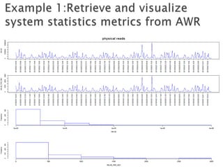
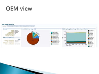
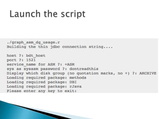
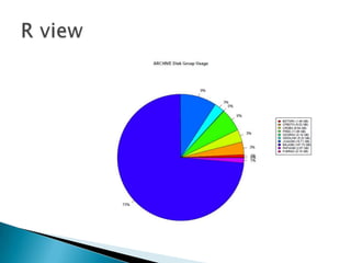
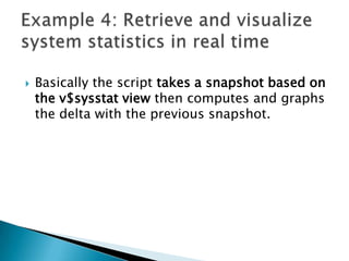
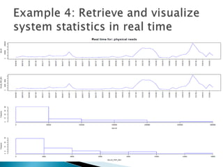
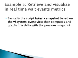
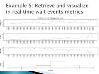
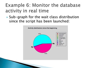
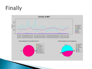
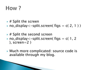
The document discusses using R to analyze and visualize Oracle database metrics and statistics in real time. It provides examples of R code to connect to an Oracle database and retrieve system statistics and wait event data. The code then computes changes from the previous snapshot and graphs metrics over time, including system statistics by interval, wait times and events, and wait class distributions. It also describes splitting the screen into multiple graphs to show various views of the real-time data. The goal is to build interactive dashboards to monitor database performance using R.

1. Bertrand Drouvot

2. 






Oracle DBA since 1999
OCP 9i,10g,11g
Rac certified Expert
Exadata certified implementation specialist
Blogger since 2012
@bertranddrouvot
BasketBall fan

3. 




Some examples of R usage with the oracle
database
From a DBA point of view
Retrieve system statistics/wait events with
some AWR queries
Real time Data
Dashboard of the database activity

4. 


R installation
R programing
R studio (powerful and productive user
interface for R)

5. 

Because R is a powerful tool for statistical
analysis with graphing and plotting packages
built in.
Furthermore, R can connect to Oracle via a
JDBC package which makes importing data
very easy.

6. 
http://www.r-project.org/

7. 



library(RJDBC)
drv <JDBC("oracle.jdbc.driver.OracleDriver","/ec/pr
od/server/oracle/olrprod1/u000/product/11.
2.0.3/jdbc/lib/ojdbc6.jar")
conn<-dbConnect(drv,conn_string,"sys as
sysasm",sys_pwd)
Data_frame<-dbGetQuery(conn,myquery)

8. select s.begin_interval_time,sta.stat_name,sta.VALUE,
round(((sta.VALUE)/
(
(extract(day from s.END_INTERVAL_TIME)-extract(day from s.BEGIN_INTERVAL_TIME))*86400 +
(extract(hour from s.END_INTERVAL_TIME)-extract(hour from s.BEGIN_INTERVAL_TIME))*3600 +
(extract(minute from s.END_INTERVAL_TIME)-extract(minute from s.BEGIN_INTERVAL_TIME))*60 +
(extract(second from s.END_INTERVAL_TIME)-extract(second from s.BEGIN_INTERVAL_TIME))
)
),2) VALUE_PER_SEC
from
(
select instance_number,snap_id,stat_name,
value - first_value(value) over (partition by stat_name order by snap_id rows 1 preceding) "VALUE"
from
dba_hist_sysstat
where stat_name like nvl('&stat_name',stat_name)
and instance_number = (select instance_number from v$instance)
) sta, dba_hist_snapshot s
where sta.instance_number=s.instance_number
and sta.snap_id=s.snap_id
and s.BEGIN_INTERVAL_TIME >= trunc(sysdate-&sysdate_nb_day_begin_interval+1)
and s.BEGIN_INTERVAL_TIME <= trunc(sysdate-&sysdate_nb_day_end_interval+1)
order by s.begin_interval_time asc;

11. 







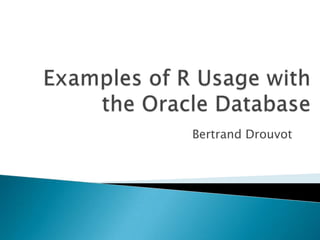
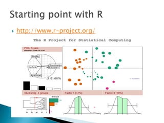
# Plot the 4 graphs
par(mfrow =c(4,1))
plot(sqstat[,'DATEEVT'],sqstat[,'VALUE'],type="l",col="blue"
,xaxt="n",main=stat_name,cex.main=2,xlab="",ylab="VAL
UE")
Axis(side=1,at=sqstat$DATEEVT,round(skip),format="%Y/
%m/%d %H:%M")
plot(sqstat[,'DATEEVT'],sqstat[,'VALUE_PER_SEC'],type="l",c
ol="blue",xaxt="n",xlab="",ylab="VALUE_PER_SEC")
Axis(side=1,at=sqstat$DATEEVT,round(skip),format="%Y/
%m/%d %H:%M")
hist(sqstat[,'VALUE'],xlab="VALUE",main=NULL,border="bl
ue")
hist(sqstat[,'VALUE_PER_SEC'],xlab="VALUE_PER_SEC",main
=NULL,border="blue")

12. select e.WAIT_CLASS,e.event_name,s.begin_interval_time,e.TOTAL_WAITS,e.TIME_WAITED_MS,e.TIME_WAITED_MS /
TOTAL_WAITS "MS_PER_WAIT"
from
(
select instance_number,snap_id,WAIT_CLASS,event_name,
total_waits - first_value(total_waits) over (partition by event_name order by snap_id rows 1 preceding)
"TOTAL_WAITS",
(time_waited_micro - first_value(time_waited_micro) over (partition by event_name order by snap_id rows 1
preceding))/1000 "TIME_WAITED_MS"
from
dba_hist_system_event
where
WAIT_CLASS like nvl('&WAIT_CLASS',WAIT_CLASS)
and event_name like nvl('&event_name',event_name)
and instance_number = (select instance_number from v$instance)
) e, dba_hist_snapshot s
where e.TIME_WAITED_MS > 0
and e.instance_number=s.instance_number
and e.snap_id=s.snap_id
and s.BEGIN_INTERVAL_TIME >= trunc(sysdate-&sysdate_nb_day_begin_interval+1)
and s.BEGIN_INTERVAL_TIME <= trunc(sysdate-&sysdate_nb_day_end_interval+1) order by 1

14. 








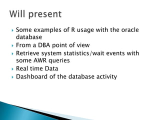
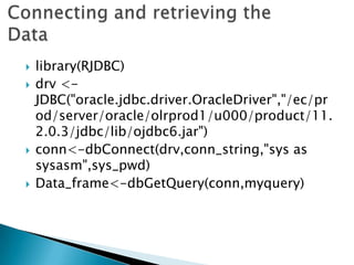
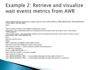
# Plot the 4 graphs
par(mfrow =c(4,1))
plot(sqevent[,'DATEEVT'],sqevent[,'TIME_WAITED_MS'],type="l",col="blue"
,xaxt="n",main=event,cex.main=2,xlab="",ylab="TIME_WAITED_MS")
Axis(side=1,at=sqevent$DATEEVT,round(skip),format="%Y/%m/%d
%H:%M")
plot(sqevent[,'DATEEVT'],sqevent[,'TOTAL_WAITS'],type="l",col="blue",xa
xt="n",xlab="",ylab="NB_WAITS")
Axis(side=1,at=sqevent$DATEEVT,round(skip),format="%Y/%m/%d
%H:%M")
plot(sqevent[,'DATEEVT'],sqevent[,'MS_PER_WAIT'],type="l",col="blue",xa
xt="n",xlab="",ylab="MS_PER_WAIT")
Axis(side=1,at=sqevent$DATEEVT,round(skip),format="%Y/%m/%d
%H:%M")
hist(sqevent[,'MS_PER_WAIT'],xlab="MS_PER_WAIT",main=NULL,border="
blue")

15. 
Query is a little bit complicated (comes from
OEM)

19. 













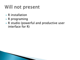
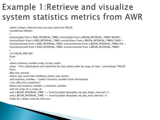
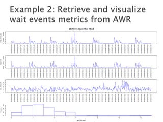
# compute percentages
pct <- round(dg_space[,'SIZE_GB']/sum(dg_space[,'SIZE_GB'])*100)
# add %
pct <- paste(pct,"%",sep="")
# Add db size to db_name
db_name_size<-paste(dg_space[,'DB_NAME']," (",sep="")
db_name_size<-paste(db_name_size,dg_space[,'SIZE_GB'],sep="")
db_name_size<-paste(db_name_size," GB)",sep="")
# Set the colors
colors<-rainbow(length(dg_space[,'DB_NAME']))
# Plot
pie(dg_space[,'SIZE_GB'], labels = pct, col=colors, main=paste(dg," Disk Group Usage",sep=""))
# Add a legend
legend(x=1.2,y=0.5,legend=db_name_size,fill=colors,cex=0.8)

20. 
Basically the script takes a snapshot based on
the v$sysstat view then computes and graphs
the delta with the previous snapshot.

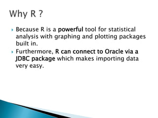
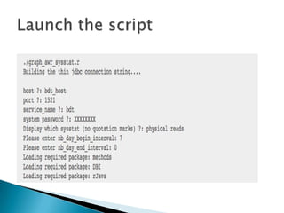
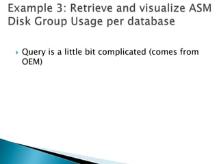
23. myquery<-"
Select to_char(sysdate,'YYYY/MM/DD HH24:MI:SS') as DATEEVT, NAME,VALUE,1 VALUE_PER_SEC
from v$sysstat
where name='"
# Keep them
prev_date<<-qoutput[,'DATEEVT']
prev_value<<-qoutput[,'VALUE']
# Launch the loop for the real-time graph
nb_refresh <- as.integer(nb_refresh)
for(i in seq(nb_refresh)) {
# Get the new data
Sys.sleep(refresh_interval)
qoutput<-dbGetQuery(conn,myquery)
# Keep the current value
current_date<-qoutput[,'DATEEVT']
current_value<-qoutput[,'VALUE']
# compute difference between snap for value and value per sec
#qoutput[,'DATEEVT']<-current_date
qoutput[,'VALUE']<-current_value-prev_value

24. 
Basically the script takes a snapshot based on
the v$system_event view then computes and
graphs the delta with the previous snapshot.

26. myquery<-"
Select to_char(sysdate,'YYYY/MM/DD HH24:MI:SS') as
DATEEVT, EVENT,TOTAL_WAITS,TIME_WAITED_MICRO/1000 as TIME_WAITED_MS,1 MS_PER_WAIT
from v$system_event
where event='"
# Keep them
prev_tw<<-qoutput[,'TIME_WAITED_MS']
prev_twaits<<-qoutput[,'TOTAL_WAITS']
# So we want 4 graphs
par(mfrow =c(4,1))
# Launch the loop for the real-time graph
nb_refresh <- as.integer(nb_refresh)
for(i in seq(nb_refresh)) {
# Get the new data
Sys.sleep(refresh_interval)
qoutput<-dbGetQuery(conn,myquery)
# compute difference between snap for time_waited_ms, total_waits and then compute ms_per_wait
qoutput[,'TIME_WAITED_MS']<-current_tw-prev_tw
qoutput[,'TOTAL_WAITS']<-current_twaits-prev_twaits

27. myquery<-"
select to_char(sysdate,'YYYY/MM/DD HH24:MI:SS') as DATEEVT,
wait_class as WAIT_CLASS,
time_waited_micro/1000 as TIME_WAITED_MS,
EVENT as EVENT
from v$system_event where WAIT_CLASS != 'Idle'
union
select to_char(sysdate,'YYYY/MM/DD HH24:MI:SS') as DATEEVT,
'CPU' as WAIT_CLASS
,sum(value/1000) as TIME_WAITED_MS
,'CPU' as EVENT
from
v$sys_time_model
where
stat_name IN ('background cpu time', 'DB CPU')
"

29. 
Sub-graph for the time waited (in ms) per
wait class:

30. 
Sub-graph for the wait events distribution
of the wait class having the max time
waited during the last snap:

31. 
Sub-graph for the wait class distribution
since the script has been launched:

33. 




# Split the screen
no_display<-split.screen( figs = c( 2, 1 ) )
# Split the second screen
no_display<-split.screen( figs = c( 1, 2
), screen=2 )
Much more complicated: source code is
available through my blog.

34. 

Retrieve and visualize in real time the output
of my asm_metrics.pl utility.
What is yours ?