Error entropy minimization for brain image registration using hilbert huang transform and echo state neural network

IJRET: International Journal of Research in Engineering and Technology eISSN: 2319-1163 | PISSN: 2321-7308
_______________________________________________________________________________________
Volume: 03 Special Issue: 07 | May-2014, Available @ http://www.ijret.org 859
ERROR ENTROPY MINIMIZATION FOR BRAIN IMAGE REGISTRATION USING HILBERT-HUANG TRANSFORM AND ECHO STATE NEURAL NETWORK Rajeswari R1, Anthony Irudhayaraj A2, Purushothaman S3 1Research scholar, Department of computer science, Mother Teresa Women's University, Kodaikanal, India 2Dean, Information Technology, Arupadai Veedu Institute of Technology, Paiyanoor-6031104, India 3Professor, PET Engineering College, Vallioor-627117, India Abstract This paper presents the work on functional magnetic resonance imaging slice registration. Hilbert-Huang transform is used to extract the features of the source image slice and target image slice. The features are used as inputs for the echo state neural network (ESNN) which is recurrent neural network. The training of ESNN is carried out by changing the different number of reservoirs in the hidden layer that result in minimum error between floating and target image slice after registration. Statistical features of the decomposed signals of the source and target image slices are used in the input layer of ESNN. The accuracy of the registration is high. Keywords— Echo state neural network (ESNN), Empirical Mode Decomposition (EMD), Hilbert Transform (HT), Hilbert-Huang transform (HHT), Image alignment, Medical image registration, Processing element
--------------------------------------------------------------------***------------------------------------------------------------------ 1. INTRODUCTION Image registration is an important requirement in medical imaging. Image registration is the most important step of image fusion task [Yang-Ming Zhu, 14]. Image fusion is used to combine images obtained from different imaging modalities [Woei-Fuh Wang et al., 12]. With increase in a number of imaging techniques and imaging sensors, many modalities are used for image registration. More detailed information can be obtained with many modalities and com- plete characterization of the image anatomies and functional properties are attainable. The analysis of multiple acquisi- tions of the same subject, comparisons of images across subjects or groups of subjects are done by the doctors. The medical experts rely on manual comparisons of images, but the abundance of information available makes this task difficult. Automatic processing of the images is required which produce a summary and potentially a visual display of all the available information relevant to the examined body parts. 2 RELATED WORKS The image analysis system is presented [Liao et al., 5] for SPECT images that perform a series of image processing procedures including 3D image registration, gray level normalization, and brain extraction, which map all the 3D brain data to the same space for further analysis.
The aligned images undertake a standard statistical analysis. One such method is a paired t test. This is used to detect the areas in the images with significant deviations. A method is proposed [Cao, 2004] that involves repeated iteration that considers closeness. The algorithm shows closest point map on a regular grid that introduces a registration error.
Registration is described [Daneshvar and Ghassemian, 2] as a process to align differently acquired images of the same subject. Automated registration of CT and MR head images is studied. It is assumed that images are only of relative translation and rotation. An automatic method to register CT and magnetic resonance (MR) brain images by using first principal directions of feature images is [Lifeng Shang et al., 6] used. The goal of the registration is to find the optimal transformation [Shaoyan sun et al., 8]. Mutual information (MI) is used as a similarity measure when the two images matches [Yongsheng Du et al., 13]. A measure is used and tested on magnetic resonance (MR) and CT images [Dejan Tomazevic et al., 3]. The measure is tested on different images considered for registration. 3. MATERIALS Data has been collected from a standard database available in statistical parametric mapping (SPM) website. The website presents Positron emission tomography (PET) and functional magnetic resonance imaging (fMRI) data collected for single subject and multiple subjects.

_______________________________________________________________________________________
4. METHODS
4.1 Hilbert-Huang Transform (Empirical Mode De-composition
(EMD) and Hilbert Transform (HT)
The features of the image slices are extracted using HHT
[Suganthi and Purushothaman, 7]. These features are used to
train the ESNN and align the image slices. Instead of taking
the representative points of the floating image and target
image, the entire floating image is aligned with the target
image.
An image is formed from the quantized values of the conti-nuous
signals based on the intensity value recognized. The
details of frequencies, amplitude and phase contents can be
obtained by decomposition of the signal. This is possible by
using EMD followed by Hilbert Transform (HT) [Jayashree
et al., 4] and [Stuti et al., 9]. The EMD produces mono com-ponents
called intrinsic mode functions (IMFs) from the
original signal. The signal is the intensity values of a row in
the image slice. In a 64 X 64 image slice, 64 signals corres-ponding
to 64 rows and another 64 signals corresponding to
columns of the image slice are used for alignment.
Many IMFs can be present in the signal. An IMF represents
a waveform. The waveform contains a different amplitude.
Instantaneous frequency (IF) and instantaneous amplitude
(IA) are obtained by applying HT on an IMF. A signal
should be symmetric with regard to the local zero mean, and
should contain the same number of extreme and zero cross-ings.
The steps involved in EMD of a signal X(t) with harmonics
(due to the presence of noise in the image slice) into a set of
IMFs are as follows.
Step 1: All local maxima of X(t) are identified and the
points are connected using cubic spline. The interpolated
curve is obtained. The upper curve is called the upper
envelope (Maximum_envelope).
Step 2: All local minima of X(t) are identified and the points
are connected using cubic spline. The lower curve is called
the lower envelope (Minimum_envelope) obtained by cubic
spline.
Step 3: The average is computed by using equation (1):
(1)
where
a = Maximum_envelope and
b = Minimum_envelope.
Step 4: A new signal is obtained by using equation (2)
(2)
where
h11(t) is called first IMF. Subsequent IMF‟s are to be found
if there are some overshoots and undershoots in the IMF.
Hence, the envelope mean differs from the true local mean
and h11(t) becomes asymmetric.
In order to find the additional IMF‟s, h11(t) is taken as the
new signal. After nth iteration, we have equation (3):
(3)
where
M1n(t) is the mean envelope after the nth iteration and
h1(n-1)(t) is the difference between the signal and the mean
envelope at the (k-1)th iteration.
Step 5: Coarse to fine (C2F) is calculated by using equations
(4-6).
(4)
where
n IMF = final IMF obtained
n IMF
(5)
Similarly,
2
(a b)
M


h (t) X(t) M (t) 11 11  
h (t) h (t) M (t) 1n 1(n 1) 1n   
1 n C2F  IMF
2 n (n 1) C2F IMF IMF   
Table 1: Sample image slices used for image
registration

_______________________________________________________________________________________
(6)
where
C2Fn is the original signal.
Step 6: Fine to coarse (F2C) is calculated by using equations
(7-9).
(7)
(8)
(9)
where
F2Cn is the original signal.
Step 7: Hilbert transform is applied for each IMF and ana-lytical
signal is obtained. A complex signal is obtained from
each IMF by using equation (10).
Analytic (IMF) = real(IMF) + imag(IMF) (10)
Step 8: Instantaneous frequencies are obtained from analyti-cal
signal by using equation (11)
IF= [0.5x(angle(-Xanalytic(t+1)*conj(Xanalytic(t-1)))+π]/(2xπ)
(11)
Step 9: Instantaneous amplitudes are obtained from the ana-lytical
signal by using equation (12).
IA= sqrt(real(IMF)2 + imag(IMF)2 ) (12)
Feature Extraction from EMD
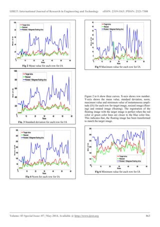
Twelve features are extracted: six features from each IF and
six features from each IA. The features are mean, standard
deviation, norm, maximum and minimum of IF. Similarly
mean, standard deviation, norm, maximum and minimum of
IA and energy of F2C and C2F waveforms of an IMF.
The features are given in equations (13-25).
V1=1/d Σ(IF) (13)
where
d is samples in a frame and
V1 is mean value of Instantaneous Frequency.
V2 =1/d Σ(IF-V1) (14)
where
V2 is standard deviation of Instantaneous Frequency.
V3=maximum (IF) (15)
V4=minimum (IF) (16)
V5=norm (IF)2 (17)
where
V5 is energy value of frequency.
V6 = 1/d Σ (IA) (18)
V7= 1/d Σ(IA-V6) (19)
where
V7 is standard deviation of Instantaneous amplitude
V8=maximum (IA) (20)
V9=minimum (IA) (21)
V10=norm (IA) 2 (22)
where
V10 is energy value of Amplitude.
V11= Σ log2 (abs(F2C))2 (23)
where
V11 is Log 2 value of F2C
V12= Σ log2 (abs(C2F))2 (24)
Where
V12 is Log 2 value of C2F. (25)
4.2 Echo State Neural Network
The ESNN is presented in Figure 1. It possesses highly in-terconnected
and recurrent topology of nonlinear processing
element (PEs). The PE contains a reservoir of rich dynamics.
PE contains information about the history of input and out-put
patterns. The outputs of the internal PEs (echo states) are
fed to a memoryless with adaptive readout network. The
memoryless readout is trained, whereas the recurrent topolo-gy
has fixed connection weights. This reduces the complexi-ty
of recurrent neural network (RNN) training to simple li-near
regression while preserving a recurrent topology. The
echo state condition is defined in terms of the spectral radius
(the largest among the absolute values of the eigenvalues of
a matrix, denoted by (|| ||) of the reservoir‟s weight matrix
(||W||<1). This condition states that the dynamics of the
ESNN is uniquely controlled by the input, and the effect of
the initial states vanishes. The recurrent network is a reser-voir
of highly interconnected dynamical components, states
of which are called echo states. The memory less linear rea-dout
is trained to produce the output.
By considering the recurrent discrete-time neural network
given in Figure 1 with „M‟ input units, „N‟ internal PEs, and
„L‟ output units, the value of the input unit at time „n‟ is u(n)
= [u1(n), u2(n), . . . , uM(n)]T,
n n (n 1) 1 C2F  IMF  IMF ....... IMF 
1 1 F2C  IMF
2 1 2 F2C  IMF  IMF
n 1 2 n F2C  IMF  IMF ....... IMF

_______________________________________________________________________________________
The internal units are
x(n)=[x1(n), x2(n), , xN(n)]T (26)
Output units are
y(n) = [y1(n), y2(n),, yL(n)]T (27)
The connection weights are given
a) in an (N x M) weight matrix
back
ij
back W  W for
connections between the input and the internal PEs,
b) in an N × N matrix
in
ij
in W  W for connections
between the internal PEs
c) in an L × N matrix
out
ij
out W  W for connections
from PEs to the output units and
d) in an N × L matrix
back
ij
back W  W for the connec-tions
that project back from the output to the internal
PEs.
The activation of the internal PEs (echo state) is updated
according to equation (28).
x(n + 1) = f(Win u(n + 1) + W X(n) +
Wback y(n)), (28)
where
f = ( f1, f2, . . . , fN) are the internal PEs‟ activation functions.
All fi‟s are hyperbolic tangent functions
x x
x x
e e
e e




. The out-put
from the readout network is computed according to
y(n + 1) = fout (Wout x(n + 1)), . (29)
where
are the output unit‟s nonli-near
functions.
Training ESNN Algorithm
The algorithm for training the ESNN is as follows:
Step 1: Read a Pattern (I) (floating image) and its Target (T)
value.
Step 2: The number of reservoirs is fixed.
Step 3: The number of nodes in the input layer = length of
pattern.
Step 4: The number of nodes in the output layer = number
of target values.
Step 5: Random weights are initialized between input and
hidden layer (Ih) hidden and output.
Step 6: Obtain S = tanh(Ih*I + Ho * T + Ho * T).
Step 7: Obtain a = Pseudo inverse (S).
Step 8: Obtain Wout = a * T and store Wout for testing.
The algorithm for testing / registration on image slice is
as follows:
Step 1: Read a Pattern (I) (floating image).
Step 2: Obtain F=Ih*I.
Step 3: TH = Ho * T.
Step 4: TT = R*S.
Step 5: S = tanh(F+TT+TH).
Step 6: a = Pseudo inverse (S).
Step 7: Estimated = a * Wout.
Step 8: Relocate the intensity values.
5. RESULTS AND DISCUSSIONS
Images have been collected from the standard database
available in SPM website. The website presents PET and
fMRI data collected for single subject and multiple subjects.
Rest condition and task related images have been presented
with realignment, co-registration, normalization, smoothing
wherever applicable.
Figures (2-11) present plots of the statistical features ob-tained
through equations (13-22).
( , ,...., ) 1 2
out
L
out out out f  f f f
Fig. 1. Schematic diagram for training ESNN with HHT
features

_______________________________________________________________________________________
Figure 2 to 6 show three curves. X-axis shows row number.
Y-axis shows the mean value, standard deviation, norm,
maximum value and minimum value of instantaneous ampli-tude
(IA) for each row for target image, resized image (float-ing)
and rotated image (floating). The registration of the
floating image with the target image is perfect when the red
color or green color lines are closer to the blue color line.
This indicates that, the floating image has been transformed
to match the target image.
Fig 2 Mean value for each row for IA
0 10 20 30 40 50 60
0
20
40
60
80
100
Rows
Mean of IA
Target slice
Resized
Rotated -10degrees-floating slice
Fig. 3 Standard deviation for each row for IA
0 10 20 30 40 50 60
0
200
400
600
800
1000
Rows
Std of IA
Target slice
Resized
Fig 4 Norm for each row for IA
0 10 20 30 40 50 60
0
50
100
150
200
250
300
350
Rows
Norm of IA
Target slice
Resized
Fig 5 Maximum value for each row for IA
0 10 20 30 40 50 60
0
5
10
15
20
25
30
35
40
45
Rows
Max of IA
Target slice
Resized
Fig 6 Minimum value for each row for IA
0 10 20 30 40 50 60
50
100
150
200
250
300
350
Rows
Min of IA
Target slice
Resized

_______________________________________________________________________________________
Figure 7 to 11 show three curves. X-axis shows column
number. Y-axis shows the mean value, standard deviation,
norm, maximum value and minimum value of instantaneous
amplitude (IA) for each column for target image, resized
image (floating) and rotated image (floating).
Fig 7 Mean value for each column for IA
0 10 20 30 40 50 60
0
10
20
30
40
50
60
70
80
90
Columns
Mean of IA
Target slice
Resized
Fig 9 Norm for each column for IA
0 10 20 30 40 50 60
0
50
100
150
200
250
300
Columns
Norm of IA
Target slice
Resized
Fig 10 Maximum value for each column for IA
0 10 20 30 40 50 60
0
10
20
30
40
50
60
70
Columns
Max of IA
Target slice
Resized
Fig 11 Minimum value for each column for IA
0 10 20 30 40 50 60
50
100
150
200
250
300
350
Columns
Min of IA
Target slice
Resized
Fig 8 Standard deviation for each column for IA
0 10 20 30 40 50 60
0
200
400
600
800
1000
Columns
Std of IA
Target slice
Resized

_______________________________________________________________________________________
Figure 13 shows estimation performance for ESNN and
HHT+ESNN for vertical direction.
Figure 14 shows estimation performance of proposed algo-rithms
for Horizontal direction
Figure 15 shows estimation performance of proposed algo-rithms
for Rotation.
Figure 16 shows estimation performance of ESNN and
HHT+ESNN for CW/CCW.
5.1 Comparison of Error Entropy of Proposed Al-gorithms
Figure 17 shows error entropy of proposed algorithms for
vertical translation. The error entropy for HHT+ESNN is
minimal
vertical direction. Except ESNN, the error entropy for
HHT+ESNN is least.
horizontal translation. Except ESNN, the error entropy for
other proposed algorithms are minimal. The error entropy
for HHT+ESNN is least when compared to other proposed
algorithms.
Fig.15. Rotation estimated by proposed algorithms
1 2 3 4 5 6 7 8 9 10 11
-5
0
5
10
15
20
25
30
Patterns
Rotation
Target value
Estimated by ESNN
Estimated by HHT+ESNN
Fig.12. Vertical translation estimated by proposed algo-rithms
1 2 3 4 5 6 7 8 9 10 11
-4
-2
0
2
4
6
8
10
12
Patterns
Vertical translation
Target value
Estimated by ESNN
Fig.13. Vertical direction estimated by proposed algo-rithms
1 2 3 4 5 6 7 8 9 10 11
0
1
2
3
4
5
6
Patterns
Vertical direction
Target value
Estimated by ESNN
Fig. 14. Horizontal direction estimated by proposed al-gorithms
1 2 3 4 5 6 7 8 9 10 11
0
1
2
3
4
5
Patterns
Horizontal direction
Target value
Estimated by ESNN
Fig. 16. CW/ CCW estimated by proposed algorithms
1 2 3 4 5 6 7 8 9 10 11
-1
0
1
2
3
4
5
Patterns
CW /CCW direction
Target value
Estimated by ESNN

_______________________________________________________________________________________
horizontal direction. Except ESNN, the error entropy for
proposed algorithm is minimal.
Rotation. The error entropy for HHT+ESNN is least when
compared to ESNN algorithm.
Fig. 17. Error entropy for Vertical translation
1 2 3 4 5 6 7 8 9 10 11
0
1
2
3
4
5
6
Patterns
Error entropy
Vertical translation
Estimated by ESNN
Fig. 18 Error entropy for Vertical direction
1 2 3 4 5 6 7 8 9 10 11
0
0.5
1
1.5
2
2.5
3
3.5
4
Patterns
Error entropy
Vertical direction
Estimated by ESNN
Fig. 19 Error entropy for Horizontal translation
1 2 3 4 5 6 7 8 9 10 11
0
1
2
3
4
5
Patterns
Error entropy
Horizontal translation
Estimated by ESNN
Fig. 20. Error entropy for Horizontal direction
1 2 3 4 5 6 7 8 9 10 11
0
1
2
3
4
5
Patterns
Error entropy
Horizontal direction
Estimated by ESNN
Fig. 21. Error entropy for Rotation
1 2 3 4 5 6 7 8 9 10 11
0
5
10
15
20
Patterns
Error entropy
Rotation
Estimated by ESNN
Fig. 22. Error entropy for CW/CCW
1 2 3 4 5 6 7 8 9 10 11
0
0.5
1
1.5
2
2.5
3
3.5
4
Patterns
Error entropy
CW /CCW direction
Estimated by ESNN

_______________________________________________________________________________________
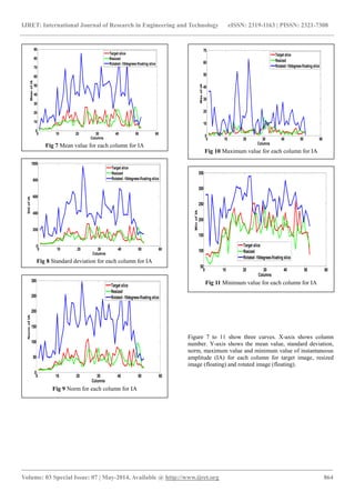
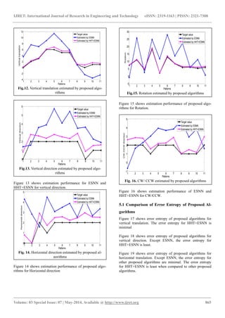
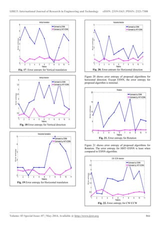
Figure 22 shows error entropy of proposed algorithms for CW/CCW. Except ESNN, the error entropy for proposed algorithm HHT+ESNN is minimal. The figures show HHT+ESNN produce least error entropy which indicates high registration accuracy. 6. CONCLUSIONS Hilbert Huang transform has been used for extracting features from the fMRI slices. These features are used as inputs for training ESNN algorithm. Using the trained information, registration of fMRI slices are done. The HHT features helps in accuracte image slice registration. REFERENCES
[1] Z.Cao, S.Pan, R.Li, R.Balachandran, J.M.Fitzpatrick, W.C.Chapman, and B.M.Dawant, “Registration of medical images using an interpolated closest point transform Method and valida- tion”, Medical Image Analysis,vol.8,pp.421- 427,2004.
[2] S.Daneshvar, and H.Ghassemian: A hybrid algorithm for medical image registration. IEEE Engi- neering Medicine Biology Society, Conference Pro- ceedings, vol. 3: pp.3272-3275, 2005.
[3] Dejan Tomazevic, Bostjan Likar, Franjo Pernus: “Multi-feature mutual information image registration”, Image analysis and stereology quantitative methods and applications; vol.31,No.10,pp.43-53, 2012
[4] T.Jayasree, D.Devaraj, and R.Sukanesh, “Power quality disturbance classification using Hilbert transform and RBF networks”, Neuro computing, vol.73, no.9, pp.1451-1456, 2010.
[5] Y.L.Liao, N.T.Chiu, C.M.Weng, and Y.N.Sun: “Registration and Normalization Techniques for As- sessing Brain Functional Images”, Biomedical Engi- neering applications Basis and Communications; vol.15, pp.87-94, 2003.
[6] Lifeng Shang, Lv Jian Cheng, Zhang Yi, “Rigid medical image registration using PCA neural network”, Neuro computing, vol.69, pp.1717-1722, 2006.
[7] S.Purushothaman and D.Suganthi, “fMRI segmentation using echo state neural network”, International Journal of Image Processing, vol. 2, no.1, pp.1-9, 2008.
[8] Shaoyan Sun, Liwei Zhang, and Chonghui Guo: “Medical Image Registration by Minimizing Diver- gence Measure Based on Tsallis Entropy”, World Academy of Science, Engineering and Technology, pp.223-228, 2006.
[9] Stuti Shukla, S. Mishra, and Bhim Singh: “Empiri- cal-Mode Decomposition with Hilbert Transform for Power-Quality Assessment”, IEEE transactions on power delivery; vol.24,no.4, pp.2159–2165, 2009.
[10] T.Suganthi and S.Purushothaman, “Segmentation Of Satellite Images Using Fuzzy Logic And Hilbert Huang Transform”, International Journal of Engi-
neering Research and Applications, vol.2, issue 2, Mar-Apr 2012, pp.1020-1023, 2012.
[11] Woei-Fuh Wang, Frank Qh Ngo1, Jyh-Cheng Chen, Ray-Ming Huang, Kuo-Liang Chou, and Ren-Shyan Liu, “Pet-Mri Image Registration and Fusion Using Artificial Neural Networks,” Biomedical Engineer- ing applications, Basis and Communications, vol.15, pp.95-99, 2003.
[12] Yongsheng Du, Anping Song, Lei Zhu, Wu Zhang: “A Mixed-Type Registration Approach in Medical Image Processing”, Biomedical Engineering and In- formatics BMEI '09, pp.1-4, 2009.
[13] Yang-Ming Zhu, “Volume Image Registration by Cross-Entropy Optimization”, IEEE Transactions on Medical Imaging, vol.21,no.2,pp.174-180,2002.

Error entropy minimization for brain image registration using hilbert huang transform and echo state neural network

More Related Content

What's hot

Viewers also liked

Similar to Error entropy minimization for brain image registration using hilbert huang transform and echo state neural network

More from eSAT Publishing House

Recently uploaded

Error entropy minimization for brain image registration using hilbert huang transform and echo state neural network