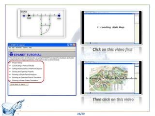
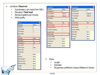
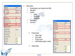
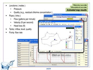
Here are the key steps for working with EPANET and ArcGIS: 1. Create a water distribution network in ArcGIS by digitizing pipes, nodes, tanks, pumps etc. and add attribute data like diameters, elevations etc. 2. Export the GIS network to an EPANET input file with coordinates and attributes. 3. Run hydraulic and water quality simulations in EPANET. 4. Import EPANET output data like pressures, flows back into ArcGIS as event themes on the map for visualization and analysis. 5. Perform further analysis like locating low pressure areas, fire flow deficiencies etc. in ArcGIS by overlaying EPANET results on the network map.

1. Waterwork Management Model :
EPANET
Jinrui Ding
학번 : 200916158
Department of Chemical Engineering

2. OUTLINE
 Introduction
 Hydraulic and Water Quality Theory
 Numerical Method
 Input Data
 Output Data
 Example Network
 ArcGIS Exercises
2/19

3. What is EPANET ?
EPANET is a computer program that performs extended period simulation of
hydraulic and water quality behavior within pressurized pipe networks.
The modeled network can consist of:
 Nodes:  Links:
• Pipe junctions • Pipes
• Storage tanks • Pumps
• Reservoirs • Valves
EPANET models:
• Flow of water in pipes • Concentration of a chemical
• Pressure at junctions • Water age
• Height of water in tanks • Source tracing
EPANET is designed to be a research tool for improving our understanding of the
movement and fate of drinking water constituents within distribution systems.
It can be used for many different kinds of applications in distribution systems analysis, such as:
 Sampling program design  Chlorine residual analysis
 Hydraulic model calibration  Consumer exposure assessment …
3/19

4. OUTLINE
 Introduction
 Hydraulic and Water Quality Theory
 Numerical Method
 Input Data
 Output Data
 Example Network
 ArcGIS Exercises
4/19

5. Hydraulic Model
A water supply distribution system consists of a complex network of interconnected
pipes, service reservoirs and pumps that deliver water from the treatment plant to a
consumer. The distribution of water through the network is governed by complex,
non-linear, non-convex and discontinuous hydraulic equations.
Two equations, which are used to determine if a network is hydraulically balanced,
are the continuity and energy equations (Eqs. (1) and (2) respectively).
The continuity equation is applied to each node with qi the flow rate (in and out of
the node) and n the number of pipes joined at the node.
The energy equation is applied to each loop in the network with hi the head loss in
each pipe and m the number of pipes in the loop. The head loss is the sum of the
local head losses and the friction head losses.
5/19

6. Water Quality
The governing equations for EPANET’s water quality solver are based on the
principles of conservation of mass coupled with reaction kinetics.
Models reactions- bulk flow and at the pipe wall
(1)
(2)
(3)
n-th order kinetics 0 / 1 order
6/19

7. OUTLINE
 Introduction
 Hydraulic and Water Quality Theory
 Numerical Method
 Input Data
 Output Data
 Example Network
 ArcGIS Exercises
7/19

8. Analysis Algorithms
 The method used in EPANET to solve the flow continuity and headloss equations that
characterize the hydraulic state of the pipe network at a given point in time can be termed a
hybrid node-loop approach —— The "Gradient Solution Method".
Assume there is a pipe network with N junction nodes and NF fixed grade nodes
(tanks and reservoirs). Let the flow-headloss relation in a pipe between nodes i and j
be given as：
(1)
The second set of equations that must be satisfied is flow continuity around all nodes:
(2)
8/19

9. The Gradient solution method begins with an initial estimate of flows in each pipe that may
not necessarily satisfy flow continuity. At each iteration of the method, new nodal heads are
found by solving the matrix equation:
(3)
After new heads are computed by solving Eq. (3), new flows are found from:
(4)
If the sum of absolute flow changes relative to the total flow in all links is larger than
some tolerance (e.g., 0.001), then Eqs. (D.3) and (D.4) are solved once again.
 EPANET’s water quality simulator uses a Lagrangian time-based approach to track the
fate of discrete parcels of water as they move along pipes and mix together at junctions
between fixed-length time steps.—— “Langrangian Transport Algorithm”
As time progresses, the size of the most
upstream segment in a pipe increases as
water enters the pipe while an equal loss
in size of the most downstream segment
occurs as water leaves the link. The size
of the segments in between these remains
unchanged.
9/19

10. OUTLINE
 Introduction
 Hydraulic and Water Quality Theory
 Numerical Method
 Input Data
 Output Data
 Example Network
 ArcGIS Exercises
10/19

11.  Junctions / Reservoir
• Coordinates ( can import from GIS )
• Elevation / Total head
• Demand (gallons per minute)
• Initial quality
 Pipes
• Length
• Diameter
• Roughness coefficient ( Hazen-Willliams C factor)
11/19

12.  Tanks data
• Coordinates ( can import from GIS)
• Elevation
• Levels
• Initial
• Minimum
• Maximum
• Diameter
• volume
 Pumps data
• Start node
• End node
• Pump curve
• Initial statue (open, close)
 Valves data
12/19

13. OUTLINE
 Introduction
 Hydraulic and Water Quality Theory
 Numerical Method
 Input Data
 Output Data
 Example Network
 ArcGIS Exercises
13/19

14.  Junctions ( nodes ) Tabular results
Graphical results
• Pressure Animated map results
• Quality (e.g., residual chlorine concentration )
 Pipes ( links )
• Flow (gallons per minute)
• Velocity (ft per second)
• Head loss (ft)
 Tanks: inflow, level, quality
 Pump: flow rate
14/19

15. OUTLINE
 Introduction
 Hydraulic and Water Quality Theory
 Numerical Method
 Input Data
 Output Data
 Example Network
 ArcGIS Exercises
15/19

16. 16/19

17. OUTLINE
 Introduction
 Hydraulic and Water Quality Theory
 Numerical Method
 Input Data
 Output Data
 Example Network
 ArcGIS Exercises
17/19

18. 1. Working with geographic features 2. Working with tables
3. Editing features 4. Working with map elements