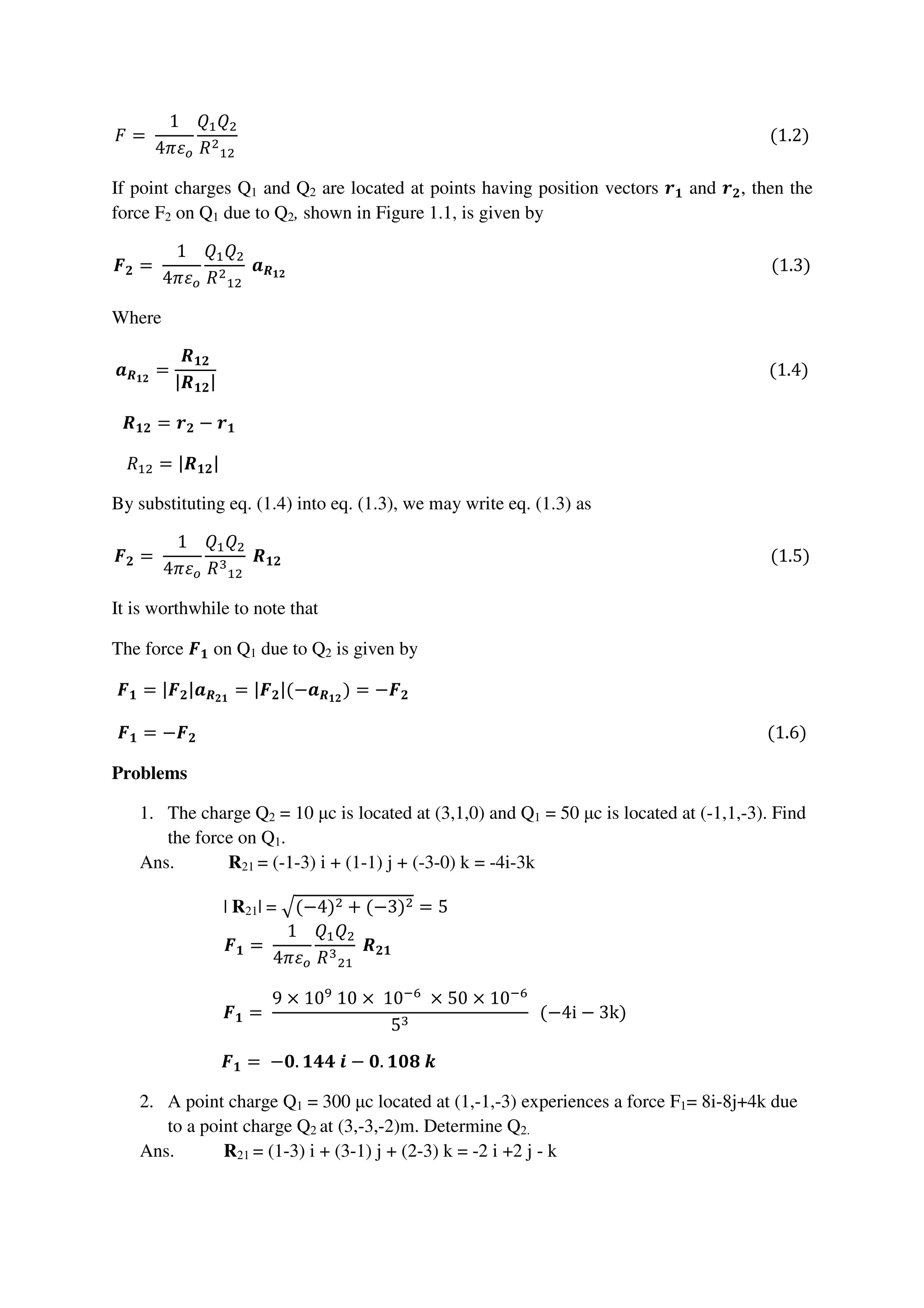
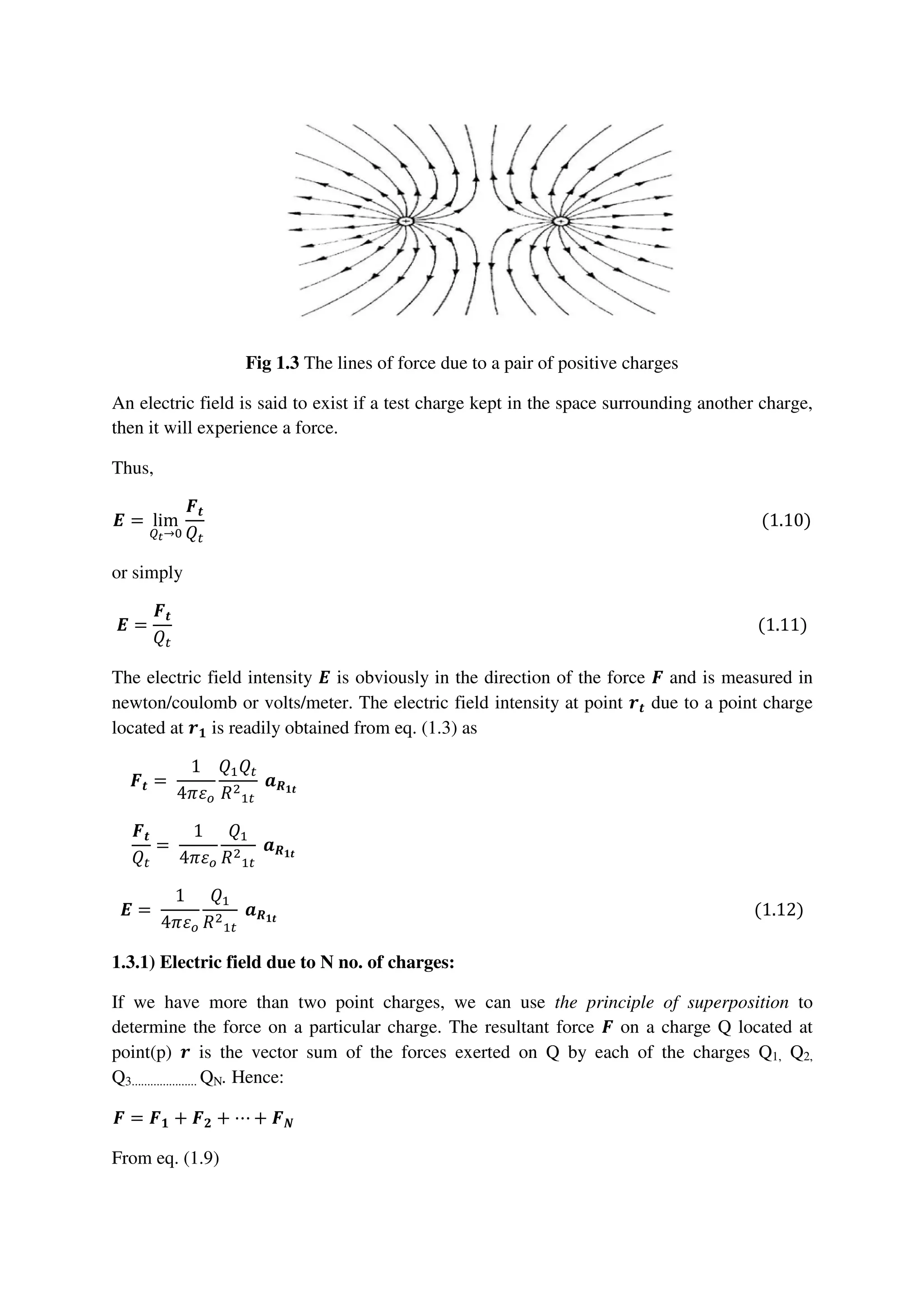
1. Coulomb's law states that the electrostatic force between two point charges is directly proportional to the product of the charges and inversely proportional to the square of the distance between them. 2. The electric field intensity is defined as the force per unit charge. The electric field intensity due to a single point charge is calculated using Coulomb's law. For multiple point charges, the total electric field is calculated using the principle of superposition. 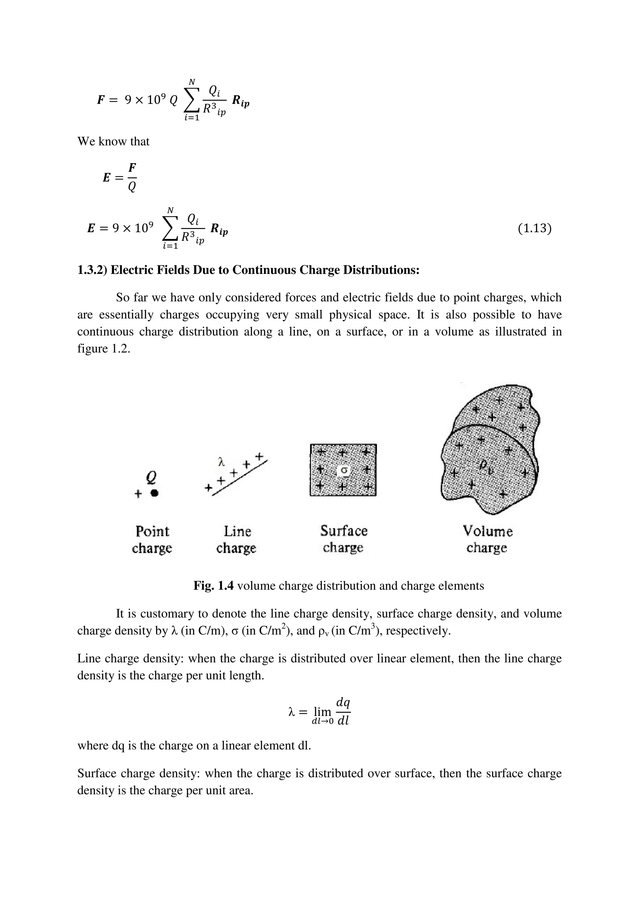3. Continuous charge distributions can also produce electric fields. These include line charge distributions with linear charge density, surface charge distributions with surface charge density, and volume charge distributions with volume charge density. The electric field due to a uniform line charge distribution can be calculated by treating

1. UNIT - I
ELECTROSTATICS
Introduction
Charges at rest produce Static Electric Field or Electrostatic field.
Field: It is the existing space in particular area due to some elements.
1.1) Coulomb’s Law
Coulomb stated that the force between two point charges separated in a vacuum or free space
by a distance which is large compared to their size is
(i) proportional to the charge on each
(ii) inversely proportional to the square of the distance between them
(iii) directed along the line joining the charges
‫ ߙ ܨ‬
ܳଵܳଶ
ܴଶ
ଵଶ
Fig. 1.1 If Q1 and Q2 have like signs the vector force ࡲ૛ on Q2 is in the same direction as ࡾ૚૛
‫ܨ‬ = ݇
ܳଵܳଶ
ܴଶ
ଵଶ
(1.1)
Where Q1 and Q2 are the positive or negative quantities of charge, R12 is the separation, and k
is proportionality constant. If the International System of Units (SI) is used. In SI units,
charges Q1 and Q2 are in coulombs (C), the distance R12 is in meters (m), and the force F is in
newtons (N) so that k = 1/4πεo. The constant εo is known as the permittivity of free space (in
farads per meter) and has the value
εo= 8.854×10-12
≈
ଵ଴షవ
ଷ଺గ
F/m
k = 1/(4πεo) = 9 × 109
m/F
Thus Eq. (1.1) becomes

2. ‫ܨ‬ =
1
4ߨߝ௢
ܳଵܳଶ
ܴଶ
ଵଶ
(1.2)
If point charges Q1 and Q2 are located at points having position vectors ࢘૚ and ࢘૛, then the
force F2 on Q1 due to Q2, shown in Figure 1.1, is given by
ࡲ૛ =
1
4ߨߝ௢
ܳଵܳଶ
ܴଶ
ଵଶ
ࢇࡾ૚૛
(1.3)
Where
ࢇࡾ૚૛
=
ࡾ૚૛
|ࡾ૚૛|
(1.4)
ࡾ૚૛ = ࢘૛ − ࢘૚
ܴଵଶ = |ࡾ૚૛|
By substituting eq. (1.4) into eq. (1.3), we may write eq. (1.3) as
ࡲ૛ =
1
4ߨߝ௢
ܳଵܳଶ
ܴଷ
ଵଶ
ࡾ૚૛ (1.5)
It is worthwhile to note that
The force ࡲ૚ on Q1 due to Q2 is given by
ࡲ૚ = |ࡲ૛|ࢇࡾ૛૚
= |ࡲ૛|(−ࢇࡾ૚૛
) = −ࡲ૛
ࡲ૚ = −ࡲ૛ (1.6)
Problems
1. The charge Q2 = 10 µc is located at (3,1,0) and Q1 = 50 µc is located at (-1,1,-3). Find
the force on Q1.
Ans. R21 = (-1-3) i + (1-1) j + (-3-0) k = -4i-3k
| R21| = ඥ(−4)ଶ + (−3)ଶ = 5
ࡲ૚ =
1
4ߨߝ௢
ܳଵܳଶ
ܴଷ
ଶଵ
ࡾ૛૚
ࡲ૚ =
9 × 10ଽ
10 × 10ି଺
× 50 × 10ି଺
5ଷ
(−4i − 3k)
ࡲ૚ = −૙. ૚૝૝ ࢏ − ૙. ૚૙ૡ ࢑
2. A point charge Q1 = 300 µc located at (1,-1,-3) experiences a force F1= 8i-8j+4k due
to a point charge Q2 at (3,-3,-2)m. Determine Q2.
Ans. R21 = (1-3) i + (3-1) j + (2-3) k = -2 i +2 j - k

3. | R21| = ඥ(−2)ଶ + (2)ଶ + (−1)ଶ = 3
ࡲ૚ =
1
4ߨߝ௢
ܳଵܳଶ
ܴଷ
ଶଵ
ࡾ૛૚
(8i − 8j + 4k ) =
9 × 10ଽ
ܳଶ × 300 × 10ି଺
3ଷ
(−2 i + 2 j − k)
Q2 = -40 µc.
1.2) Force due to N no. of charges:
If we have more than two point charges, we can use the principle of superposition to
determine the force on a particular charge. The principle states that if there are N charges Q1,
Q2, Q3..................... QN located, respectively, at points with position vectors
࢘૚, ࢘૛, ࢘૜ … … … … … ࢘ࡺ , the resultant force ࡲ on a charge Q located at point(p) ࢘ is the
vector sum of the forces exerted on Q by each of the charges Q1, Q2, Q3..................... QN. Hence:
ࡲ = ࡲ૚ + ࡲ૛ + ⋯ + ࡲࡺ
ࡲ =
1
4ߨߝ௢
ܳܳଶ
ܴଷ
ଵ௣
ࡾ૚࢖ +
1
4ߨߝ௢
ܳܳଶ
ܴଷ
ଶ௣
ࡾ૛࢖ + ⋯ +
1
4ߨߝ௢
ܳܳଶ
ܴଷ
ே௣
ࡾࡺ࢖ (1.7)
ࡲ =
ܳ
4ߨߝ௢
෍
ܳ௜
ܴଷ
௜௣
ࡾ࢏࢖
ே
௜ୀଵ
(1.8)
ࡲ = 9 × 10ଽ
ܳ ෍
ܳ௜
ܴଷ
௜௣
ࡾ࢏࢖
ே
௜ୀଵ
(1.9)
Problems
1. Find the force on a 100 µc charge at (0,0,3)m. If four like charges of 20 µc are located
on x and y axes at ±4m.
Ans. R1p = (0-4) i + (0-0) j + (3-0) k = -4 i +3 k
| R1p| = ඥ(−4)ଶ + (3)ଶ = 5
R2p = (0-0) i + (0-4) j + (3-0) k = -4 j +3 k
| R2p| = ඥ(−4)ଶ + (3)ଶ = 5
R3p = (0+4) i + (0-0) j + (3-0) k = 4 i +3 k

4. | R3p| = ඥ(4)ଶ + (3)ଶ = 5
R4p = (0-0) i + (0+4) j + (3-0) k = 4 i +3 k
| R4p| = ඥ(4)ଶ + (3)ଶ = 5
ࡲ = 9 × 10ଽ
ܳ ෍
ܳ௜
ܴଷ
௜௣
ࡾ࢏࢖
ே
௜ୀଵ
ࡲ =
9 × 10ଽ
100 × 10ି଺
× 20 × 10ି଺
5ଷ
(−4 i + 3 k − 4 i + 3 k + 4 i + 3 k + 4 i + 3 k)
ࡲ = ૚. ૠ૛ ࡷ ܰ
2. Two small diameter 10 gm dielectric balls can slide freely on a vertical plastic channel. Each
ball carries a negative charge of 1 nc. Find the separation between the balls if the upper ball is
restrained from moving.
Ans. Gravitational force and coulomb force must be equal
F2 = mg = 10 × 10-3
× 9.8 = 9.8× 10-2
N.
‫ܨ‬ଵ =
1
4ߨߝ௢
ܳܳଶ
ܴଶ
ଵ௣
Therefore F1 = F2
9.8× 10-2
=
ଽ×ଵ଴వ (ଵ× ଵ଴షల)మ
ோమ
R=0.302 m
1.3) Electric Field Intensity or Electric Field Strength (ࡱ):
It is the force per unit charge when placed in electric field.
Fig 1.2 The lines of force due to a pair of charges, one positive and the other negative

5. Fig 1.3 The lines of force due to a pair of positive charges
An electric field is said to exist if a test charge kept in the space surrounding another charge,
then it will experience a force.
Thus,
ࡱ = lim
ொ೟→଴
ࡲ࢚
ܳ௧
(1.10)
or simply
ࡱ =
ࡲ࢚
ܳ௧
(1.11)
The electric field intensity ࡱ is obviously in the direction of the force ࡲ and is measured in
newton/coulomb or volts/meter. The electric field intensity at point ࢚࢘ due to a point charge
located at ࢘૚ is readily obtained from eq. (1.3) as
ࡲ࢚ =
1
4ߨߝ௢
ܳଵܳ௧
ܴଶ
ଵ௧
ࢇࡾ૚࢚
ࡲ࢚
ܳ௧
=
1
4ߨߝ௢
ܳଵ
ܴଶ
ଵ௧
ࢇࡾ૚࢚
ࡱ =
1
4ߨߝ௢
ܳଵ
ܴଶ
ଵ௧
ࢇࡾ૚࢚
(1.12)
1.3.1) Electric field due to N no. of charges:
If we have more than two point charges, we can use the principle of superposition to
determine the force on a particular charge. The resultant force ࡲ on a charge Q located at
point(p) ࢘ is the vector sum of the forces exerted on Q by each of the charges Q1, Q2,
Q3..................... QN. Hence:
ࡲ = ࡲ૚ + ࡲ૛ + ⋯ + ࡲࡺ
From eq. (1.9)

6. ࡲ = 9 × 10ଽ
ܳ ෍
ܳ௜
ܴଷ
௜௣
ࡾ࢏࢖
ே
௜ୀଵ
We know that
ࡱ =
ࡲ
ܳ
ࡱ = 9 × 10ଽ
෍
ܳ௜
ܴଷ
௜௣
ࡾ࢏࢖
ே
௜ୀଵ
(1.13)
1.3.2) Electric Fields Due to Continuous Charge Distributions:
So far we have only considered forces and electric fields due to point charges, which
are essentially charges occupying very small physical space. It is also possible to have
continuous charge distribution along a line, on a surface, or in a volume as illustrated in
figure 1.2.
Fig. 1.4 volume charge distribution and charge elements
It is customary to denote the line charge density, surface charge density, and volume
charge density by λ (in C/m), σ (in C/m2
), and ρv (in C/m3
), respectively.
Line charge density: when the charge is distributed over linear element, then the line charge
density is the charge per unit length.
λ = lim
ௗ௟→଴
݀‫ݍ‬
݈݀
where dq is the charge on a linear element dl.
Surface charge density: when the charge is distributed over surface, then the surface charge
density is the charge per unit area.

7. σ = lim
ௗ௦→଴
݀‫ݍ‬
݀‫ݏ‬
where dq is the charge on a surface element ds.
Volume charge density: when the charge is confined within a volume, then the volume
charge density is the charge per unit volume.
ρ୴
= lim
ௗ௩→଴
݀‫ݍ‬
݀‫ݒ‬
where dq is the charge contained in a volume element dv.
1.3.3) Electric field due to line charge:
Consider a uniformly charged wire of length L m, the charge being assumed to be
uniformly distributed at the rate of λ (linear charge density) c/m. Let P be any point at which
electric field intensity has to be determined.
Consider a small elemental length dx at a distance x meters from the left end
of the wire, the corresponding charge element is λ dx. Divide the wire into a large number of
such small elements, each element will render its contribution towards the production of field
at P.
Fig 1.5 Evaluation E due to line charge
Let dE be field due to the charge element λ dx. It has a component dEx along x-axis
and dEy along y-axis.
dE = dEx ax + dEy ay

8. we know that
݀‫ܧ‬ =
λ dx
4ߨߝ௢‫ݎ‬ଶ
(1.14)
From figure 1.5 we can write,
dEx = dE cosߠ (1.15)
dEy = dE sinߠ (1.16)
Therefore we can write,
݀‫ܧ‬௫ =
λ cosθ dx
4ߨߝ௢‫ݎ‬ଶ
(1.17)
݀‫ܧ‬௬ =
λ sinθ dx
4ߨߝ௢‫ݎ‬ଶ
(1.18)
Substituting eqs. (1.17) and (1.18) in dE we get,
݀ࡱ =
λ cosθ dx
4ߨߝ௢‫ݎ‬ଶ
ࢇ࢞ +
λ sinθ dx
4ߨߝ௢‫ݎ‬ଶ
ࢇ࢟ (1.19)
From figure 1.5 we write
L1-x = h cotߠ (1.20)
-dx = -h cosec2
ߠ dߠ
(1.21)
r = h cosecߠ
(1.22)
Substituting equations (1.20), (1.21) and (1.22) in 1.19, we get
݀ࡱ =
λ cosθ dθ
4ߨߝ௢ℎ
ࢇ࢞ +
λ sinθ dθ
4ߨߝ௢ℎ
ࢇ࢟ (1.23)
The electric field intensity E due to whole length of the wire
ࡱ = න ݀ࡱ ݀ߠ
ࣂୀ࣊ିࢻ૛
ࣂୀࢻ૚
ࡱ = න ൤
λ cosθ dθ
4ߨߝ௢ℎ
ࢇ࢞ +
λ sinθ dθ
4ߨߝ௢ℎ
ࢇ࢟ ൨ ݀ߠ
ࣂୀ࣊ିࢻ૛
ࣂୀࢻ૚

9. ࡱ =
ߣ
4ߨߝ௢ℎ
ൣ‫ࢇ ߠ݊݅ݏ‬࢞ − ܿ‫ࢇ ߠݏ݋‬࢟൧
ࢻ૚
࣊ିࢻ૛
ࡱ =
ߣ
4ߨߝ௢ℎ
ൣ(‫ߙ݊݅ݏ‬ଶ − ‫ߙ݊݅ݏ‬ଵ)ࢇ࢞ + (ܿ‫ߙݏ݋‬ଶ + ܿ‫ߙݏ݋‬ଵ) ࢇ࢟൧
ܰ
‫ܥ‬
(1.24)
Case (i)
If P is the midpoint, α1= α2 = α
ࡱ =
ߣ
4ߨߝ௢ℎ
ൣ(‫ߙ ݊݅ݏ‬ − ‫ࢇ)ߙ ݊݅ݏ‬࢞ + (ܿ‫ߙ ݏ݋‬ + ܿ‫ࢇ )ߙ ݏ݋‬࢟൧
ܰ
‫ܥ‬
ࡱ =
ߣ
4ߨߝ௢ℎ
ൣ2 ܿ‫ࢇ ߙ ݏ݋‬࢟൧
ܰ
‫ܥ‬
ࡱ =
ߣ
2ߨߝ௢ℎ
ܿ‫ࢇ ߙ ݏ݋‬࢟
ܰ
‫ܥ‬
(1.25)
The direction of electric field intensity is normal to the line charge. The electric field is not
normal to the line charge if the point is not at midpoint.
Case (ii)
As length tends to
α1 = 0 and α2 = 0
from equation (1.24), we get
ࡱ =
ߣ
2ߨߝ௢ℎ
ࢇ࢟
ܰ
‫ܥ‬
(1.26)
1.3.4) Electrical field due to charged ring:
A circular ring of radius a carries a uniform charge λ C/m and is placed on the xy-plane with
axis the same as the z-axis as shown in figure.
Let dE be the electric field intensity due to a charge dQ. The ring is assumed to be formed by
several point charges. When these vectors are resolved, radial components get cancelled and
normal components get added. Therefore the direction of electric field intensity is normal to
the plane of the ring. The sum of normal components can be written as
∞

10. Fig. 1.6 charged ring
ࡱ = න ݀‫ࢇ ߙݏ݋ܿ ܧ‬ࢠ
ࡱ = න
݀ܳ
4ߨߝ௢ܴଶ
ܿ‫ࢇ ߙ ݏ݋‬ࢠ
ࡱ = න
ߣ ݈݀
4ߨߝ௢ܴଶ
ℎ
ܴ
ࢇࢠ
ࡱ =
ߣ ℎ
4ߨߝ௢ܴଷ
ࢇࢠ න ݈݀
ࡱ =
ߣ ℎ
4ߨߝ௢ܴଷ
× 2ߨܽ ࢇࢠ
ࡱ =
ߣ ℎ
4ߨߝ௢√ܽଶ + ℎଶ
ଷ × 2ߨܽ ࢇࢠ
ࡱ =
ߣ ܽ ℎ
2ߝ௢(ܽଶ + ℎଶ)ଷ/ଶ
ࢇࢠ
N
C
(1.27)

11. 1.3.5) Electrical field due to a charged disc:
A disc of radius ‘a’ meters is uniformly charged with a charged density σ c/m2
. It is required
to determine the electric field at ‘P’ which is at a distance h meters from the centre of the disc
as shown in figure 1.7
Fig. 1.7 charged disc
The disc is assumed to be formed by several rings of increasing radius. Consider a ring of
radius x meters. Each ring is assumed to be formed by number of point charges.
Let dE1 be the electric field intensity due to a charge dQ1 and dE2 is the electric field intensity
due to a charge dQ2.
Electric field due to one ring be obtained by adding normal components of dE1, dE2 .......
dEn.
Therefore
dE = (dE1 cosߠ + dE2 cosߠ + ....... + dEn cosߠ ) az
dE = (dE1 + dE2 + ....... + dEn) cosߠ az
dE = (
ௗொభ
ସగఌ௥మ +
ௗொమ
ସగఌ௥మ + ....... +
ௗொ೙
ସగఌ௥మ) cosߠ az
dE =
ௗொభାௗொమା⋯ାௗொ೙
ସగఌ௥మ cosߠ az
dE =
ௗொ
ସగఌ௥మ cosߠ az
The total charge of the ring is σ ds which is equal to dQ

12. dE =
σ ୢୱ
ସగఌ௥మ
cosߠ az (1.28)
ds = π[(x + dx)2
– x2
]
ds = π[x2
+ dx2
+ 2xdx – x2
] = 2π x dx (neglecting dx2
term)
Substituting ds in eq. (1.28) , we get
dE =
σ ଶπ୶ୢ୶
ସగఌ௥మ cosߠ az
dE =
σ ୶ୢ୶
ଶఌ௥మ
cosߠ az (1.29)
From above figure we can write
Tanߠ = x/h
x = h tanߠ
(1.30)
dx = h sec2
ߠ dߠ
(1.31)
cosߠ = h/r
r = h/ cosߠ = h secߠ
(1.32)
Substituting eqs. (1.30), (1.31) and (1.32) in (1.29) we get,
dE =
σ ( ୦ ୲ୟ୬θ)(୦ ୱୣୡమθ ୢθ)
ଶఌ୦ ୱୣୡθమ cosߠ az
dE =
σ
ଶఌ
sinߠ dߠ az
On integrating
ࡱ =
ߪ
2ߝ
න ‫ߠ݊݅ݏ‬
ఈ
଴
݀ߠ ࢇࢠ
ࡱ =
ߪ
2ߝ
ሾ−ܿ‫ߠݏ݋‬ሿ଴
ఈ
ࢇࢠ
ࡱ =
ߪ
2ߝ
(1 − ܿ‫ࢇ)ߙݏ݋‬ࢠ (1.33)
From figure 1.7
ܿ‫ߙݏ݋‬ =
ℎ
ඥ(ܽଶ + ℎଶ)

13. ∴ ࡱ =
ߪ
2ߝ
ቆ1 −
ℎ
ඥ(ܽଶ + ℎଶ)
ቇ ࢇࢠ
ܰ
‫ܥ‬
(1.34)
For infinite disc, radius ‘a’ tends to infinite and α = 90.
ࡱ =
ߪ
2ߝ
(1 − ܿ‫ࢇ)09 ݏ݋‬ࢠ
ࡱ =
ߪ
2ߝ
ࢇࢠ
ܰ
‫ܥ‬
‫ݎ݋‬
ܸ
݉
(1.35)
From equation (1.35), it can be seen that electric field due to infinite disc is independent of
distance. Electric field is uniform.
Problems
1. Determine the magnitude of electric field at a point 3 cm away from the mid point of
two charges of 10-8
c and -10-8
c kept 8 cm apart as shown in figure.
Ans. Er = 2 |E| cos ߠ
|E1|=|E2|=E
‫ܧ‬ =
1
4ߨߝ௢
ܳ
ܴଶ
‫ܧ‬ =
1
4ߨ 8.854 × 10ିଵଶ
10ି଼
0.05ଶ
= 36 ‫ ݉/ܸ ܭ‬
Er = 2 36 × 103
cos 53.1 = 57.6 K V
2. A uniform charge distribution infinite in extent lies along z-axis with a charge density
of 20 nc/m. Determine electric field intensity at (6,8,0).
Ans. d = (6-0)i+(8-0)j+0 k = 6i + 8j
d= ඥ(6ଶ + 8ଶ) = 10
ࡱ =
ߣ
2ߨߝ௢݀
ࢇࢊ
ܰ
‫ܥ‬
ࡱ =
20 × 10ିଽ
2ߨ 8.854 × 10ିଵଶ 10
6i + 8j
10
E = 21.57i + 28.76j N/C
3. A straight wire has an uniformly distributed charge of 0.3×10-4
c/m and of length 12
cm. Determine the electric field at a distance of 3 cm below the wire and displaced 3
cm to the right beyond one end as shown in figure.
Ans. tan α1 =
஼௉
஺஼
=
଴.଴ଷ
଴.ଵଶା଴.଴ଷ
=
଴.଴ଷ
଴.ଵହ

14. α1 = tan-1
(0.03/0.15)= 11.3o
tan β = 0.03/0.03 = 1
β = 45o
,
α2 = 180-45= 135o
ࡱ =
ߣ
4ߨߝ௢ℎ
ൣ(‫ߙ݊݅ݏ‬ଶ − ‫ߙ݊݅ݏ‬ଵ)ࢇ࢞ + (ܿ‫ߙݏ݋‬ଶ + ܿ‫ߙݏ݋‬ଵ) ࢇ࢟൧
ࡱ =
9 × 10ଽ
× 0.3 × 10ିସ
0.03
ൣ(sin 135 − sin 11.3)ࢇ࢞ + (cos 135 + cos 11.3) ࢇ࢟൧
ࡱ = 4.59 × 10଺
ࢇ࢞ + 2.4 × 10଺
ࢇ࢟
ࡱ = ൫4.59 ࢇ࢞ + 2.4 ࢇ࢟൯ ‫ ݉/ݒܭ‬
4. Find the force on a point charge 50 µc at (0,0,5) m due to a charge 0f 500π µc. It is
uniformly distributed over a circular disc of radius 5 m.
Ans. ߪ =
ொ
గ ௔మ
ߪ =
500π 10ି଺
ߨ 5ଶ
= 20 µ c/m
ࡱ =
ߪ
2ߝ
(1 − ܿ‫ࢇ)ߙݏ݋‬ࢠ
ࡱ =
20 × 10ି଺
2 × 8.854 × 10ିଵଶ
(1 − ܿ‫ࢇ )54 ݏ݋‬ࢠ
ࡱ = 3.3 × 10ହ
ࢇࢠ ܰ/‫ ܥ‬
F= E q
F = 3.3 × 10ହ
× 50 × 10ି଺
= 16.5 ܰ
F = 16.5 az N
5. A charge of 40/3 nc is distributed around a ring of radius 2m, find the electric field at
a point (0,0,5)m from the plane of the ring kept in Z=0 plane.

15. Ans. Q = 40/3 n c
ߣ =
ܳ
2 ߨ ܽ
=
40
3 × 10ିଽ
2 ߨ 2
= 1.06 × 10ିଽ
ܿ
݉
ࡱ =
ߣ ܽ ℎ
2ߝ௢‫ݎ‬ଷ
ࢇࢠ
N
C
ࡱ =
1.06 × 10ିଽ
× 2 × 5
2 × 8.854 × 10ିଵଶ × √29
ଷ ࢇࢠ
ࡱ = 3.83 ࢇࢠ ܸ
6. An infinite plane at y=3 m contains a uniform charge distribution of density 10-8
/6π
C/m2
. Determine electric field at all points.
Ans. (i) y>3
E = σ/2ϵ j = 10-8
/(2×6π×8.854×10-12
) j = 29.959 j
Magnitude of electric field at all points is same since the electric field due to an
infinite plane (or) disc is uniform.
For y<3
E = -29.959 j
For y<3, electric field is directed along negative y-axis. Unit vector along negative y-
direction is –j.
7. A straight line of charge of length 12 cm carries a uniformly distributed charge of
0.3×10-6
coulombs per cm length. Determine the magnitude and direction of the
electric field intensity at a point
(i) Located at a distance of a 3 cm above the wire displaced 3 cm to the right of
and beyond one end.
(ii) Located at the distance of 3 cm from one end, in alignment with, but beyond
the wire.
(iii) Located at a distance of 3 cm from one end, on the wire itself.
ans.
(i) tan α1 =
஼௉
஺஼
=
଴.଴ଷ
଴.ଵଶା଴.଴ଷ
=
଴.଴ଷ
଴.ଵହ
α1 = tan-1
(0.03/0.15)= 11.3o
tan β = 0.03/0.03 = 1
β = 45o
,
α2 = 180-45= 135o

16. ࡱ =
ߣ
4ߨߝ௢ℎ
ൣ(‫ߙ݊݅ݏ‬ଶ − ‫ߙ݊݅ݏ‬ଵ)ࢇ࢞ + (ܿ‫ߙݏ݋‬ଶ + ܿ‫ߙݏ݋‬ଵ) ࢇ࢟൧
ࡱ =
9 × 10ଽ
× 0.3 × 10ିସ
0.03
ൣ(sin 135 − sin 11.3)ࢇ࢞ + (cos 135 + cos 11.3) ࢇ࢟൧
ࡱ = 4.59 × 10଺
ࢇ࢞ + 2.4 × 10଺
ࢇ࢟
ࡱ = ൫4.59 ࢇ࢞ + 2.4 ࢇ࢟൯ ‫ ݉/ݒܭ‬
(ii) consider an element dx of charge λdx at a distance x from A. The field at P due to
the positive charge element λdx is directed to the right.
ࢊࡱ =
ߣ݀‫ݔ‬
4ߨߝ௢(‫ܮ‬ + ℎ − ‫)ݔ‬ଶ
ࢇ࢞
ࡱ =
ߣ
4ߨߝ௢
න
݀‫ݔ‬
(‫ܮ‬ + ℎ − ‫)ݔ‬ଶ
ࡸ
଴
ࢇ࢞
ࡱ =
ߣ
4ߨߝ௢
൤
1
ℎ
−
1
‫ܮ‬ + ℎ
൨ ࢇ࢞
ࡱ = 9 × 10ଽ
× 0.3 × 10ିସ
൤
1
0.03
−
1
0.15
൨ ࢇ࢞
ࡱ = 7.2 × 10଺
ࢇ࢞ ࢜/࢓
(iii) Now L=AC= 6 cm = 0.06 cm
h = 0.03 m
ࡱ =
ߣ
4ߨߝ௢
൤
1
ℎ
−
1
‫ܮ‬ + ℎ
൨ ࢇ࢞
ࡱ = 9 × 10ଽ
× 0.3 × 10ିସ
൤
1
0.03
−
1
0.09
൨ ࢇ࢞

17. E = 60 ax K v/cm
1.4) Work Done:
If a point charge ‘Q’ is kept in an electric field it experience a force F in the direction of
electric field. Fa is the applied force in a direction opposite to that of F.
Let dw be the work done in moving this charge Q by a distance dl m. Total work done in
moving the point charge from ‘a’ to ‘b’ can be obtained by integration.
ܹ = න ݀‫ ݓ‬
ܹ = න ࡲࢇ ∙ ࢊ࢒
ܹ = − න ࡲ ∙ ࢊ࢒
௕
௔
(1.36)
E = F/Q
F = E Q
ܹ = − න ࡱ ܳ ∙ ࢊ࢒
௕
௔
ܹ = −ܳ න ࡱ ∙ ࢊ࢒
௕
௔
(1.37)
E = Ex ax + Ey ay + Ez az
dl = dx ax + dyay + dz az
E ∙ dl = EX dx + Ey dy + Ez dz
∴ ܹ = −ܳ න (E୶ dx + E୷ dy + E୸ dz)
(௫మ,௬మ,௭మ)
(௫భ,௬భ,௭భ)
(1.38)
Problems

18. 1. Find the work involved in moving a charge of 1 c from (6,8,-10) to (3,4,-5) in the
field E = -x i +y j –3 k.
Ans.
ܹ = −ܳ න (E୶ dx + E୷ dy + E୸ dz)
(ଷ.ସ.ିହ)
(଺,଼,ିଵ଴)
ܹ = −1 ቈන −‫ݔ݀ ݔ‬ +
ଷ
଺
න ‫ݕ݀ ݕ‬
ସ
଼
− න ‫ݖ݀ ݖ‬
ିହ
ିଵ଴
቉
ܹ = − ൥ቆ
−‫ݔ‬ଶ
2
ቇ
଺
ଷ
+ ቆ
‫ݕ‬ଶ
2
ቇ
଼
ସ
− (3‫)ݖ‬ିଵ଴
ିହ
൩
ܹ = − ൤
−9
2
+
36
2
+
16
2
−
64
2
− −15 + 30൨
W= 25.5 J
2. Find the work done in moving a point charge of -20 µc from the origin to (4,0,0) in
the field E = (x/2 + 2y) i + 2x j
Ans.
ܹ = −ܳ න (E୶ dx + E୷ dy + E୸ dz)
(௫మ,௬మ,௭మ)
(௫భ,௬భ,௭భ)
dl = d xi
ܹ = −ܳ න (E୶ dx )
(ସ,଴,଴)
(଴,଴,଴)
ܹ = 20 × 10ି଺
න ((x/2 + 2y) dx )
(ସ,଴,଴)
(଴,଴,଴)
ܹ = 20 × 10ି଺
ቆ
‫ݔ‬ଶ
4
ቇ
଴
ସ
W = 80×10-6
J
1.5) Absolute Potential:
Absolute potential is defined as the work done in moving a unit positive charge from infinite
to the point against the electric field.

19. A point charge Q is kept at an origin as shown in figure. It is required to find the potential at
‘b’ which is at distance ‘r’ m from the reference.
Consider a point R1 at a distance ‘x’ m. The small work done to move the charge from R1 to
P1 is dw. The electrical field due to a point charge Q at a distance ‘x’ mis
ࡱ = ܳ/(4ߨߝ‫ݔ‬ଶ
)
Work done = E• dx
Total work done can be obtained by integration
Work done (W) = − Q ‫׬‬ ۳ ∙ d‫ܔ‬
ୠ
ୟ
V= − 1 ‫׬‬ ۳ ∙ d‫ܔ‬
ୠ
ୟ
V = − න ۳ ∙ d‫ܔ‬
ୠ
ୟ
E = Ex ax , dl = dx ax
V = − න
ܳ
4ߨߝ‫ݔ‬ଶ
݀‫ݔ‬
ୠ
ୟ
ܸ =
ܳ
4ߨߝ‫ݎ‬
(1.39)
1.6) Potential Difference: Vab
Potential difference Vab is defined as the work done in moving a unit positive charge from ‘b’
to ‘a’.

20. Consider a point charge Q kept at the origin of a spherical co-ordinate system. The
field is always in the direction of ar. No field in the direction of ߠ and ϕ. The points ‘a’ and
’b’ are at distance ra and rb respectively as shown in figure.
Vୟୠ = − න ۳ ∙ d‫ܔ‬
ୟ
ୠ
E = Er ar , dl = dr ar
Vୟୠ = − න E୰d୰
ୟ
ୠ
Vୟୠ = − න
ܳ
4ߨߝ‫ݎ‬ଶ
d୰
୰౗
୰ౘ
Vୟୠ =
ܳ
4ߨߝ
൤
1
‫ݎ‬௔
−
1
‫ݎ‬௕
൨
Vୟୠ =
ܳ
4ߨߝ
1
‫ݎ‬௔
−
ܳ
4ߨߝ
1
‫ݎ‬௕
Vୟୠ = Vୟ − ܸ௕ (1.40)
1.6.1) Potential difference due to line charge:
The wire is uniformly charged with λ C/m. We have to find the potential difference Vab due
to this line charge. Consider a point P at a distance P from the line charge.

21. Fig. Line charge
E = Eρ aρ
dl = dρ aρ
E•dl = Eρ aρ • dρ aρ = Eρ dρ
Potential difference Vab is the work done in moving a unit +ve charge from ‘b’ to ‘a’.
Vୟୠ = − න ۳ ∙ d‫ܔ‬
ୟ
ୠ
Vୟୠ = − න Eρ dρ
ୟ
ୠ
Vୟୠ = − න
ߣ
2ߨߝߩ
dρ
ρ౗
ρౘ
Vୟୠ =
ߣ
2ߨߝ
ln
ߩ௕
ߩ௔
(1.41)
1.6.2) Potential due to charged ring:
A thin wire is bent in the form of a circular ring as shown in figure. It is uniformly charged
with a charge density λ C/m. It is required to determine the potential at height ‘h’ m from the
centre of the ring. The ring is assumed to be formed by several point charges.
Fig. Charged ring
Let dv be the potential due to the line charge element of length dl containing a charge
dQ.
݀‫ݒ‬ =
݀ܳ
4ߨߝ‫ݎ‬
݀‫ݒ‬ =
ߣ݈݀
4ߨߝ‫ݎ‬
ܸ = න
ߣ݈݀
4ߨߝ‫ݎ‬

22. ܸ =
ߣ
4ߨߝ‫ݎ‬
න ݈݀
ܸ =
ߣ
4ߨߝ‫ݎ‬
2ߨܽ
ܸ =
ߣܽ
2ߝ‫ݎ‬
ܸ =
ߣܽ
2ߝ√ܽଶ + ܾଶ
‫)24.1( ݏݐ݈݋ݒ‬
1.6.3) Potential due to a charged disc:
let dv be the potential due to one ring. Each ring is assumed to be having several point
charges dQ1, dQ2, ............ dQn. Potential due to the ring is the sum of potential.
Fig. Charge disc
݀‫ݒ‬ =
݀ܳଵ
4ߨߝ‫ݎ‬
+
݀ܳଶ
4ߨߝ‫ݎ‬
+ … … … … … . +
݀ܳ௡
4ߨߝ‫ݎ‬
݀‫ݒ‬ =
݀ܳଵ + ݀ܳଶ + … … . . + ݀ܳ௡
4ߨߝ‫ݎ‬
݀‫ݒ‬ =
݀ܳ
4ߨߝ‫ݎ‬
݀‫ݒ‬ =
ߪ ݀‫ݏ‬
4ߨߝ‫ݎ‬
=
ߪ 2ߨ‫ݔ݀ ݔ‬
4ߨߝ‫ݎ‬
=
ߪ ‫ݔ݀ ݔ‬
2ߝ‫ݎ‬
Potential due to entire disc can be obtained by integration
ܸ = න ݀‫ݒ‬ = න
ߪ ‫ݔ݀ ݔ‬
2ߝ‫ݎ‬
௔
଴
=
ߪ
2ߝ
න
‫ݔ‬
√‫ݔ‬ଶ + ℎଶ
௔
଴
݀‫ ݔ‬
Let ‫ݔ‬ଶ
+ ℎଶ
= ‫ݐ‬ଶ
2x dx = 2t dt
Therefore we have

23. ܸ =
ߪ
2ߝ
න
‫ݐ݀ ݐ‬
‫ݐ‬
√௔మା௛మ
௛
ܸ =
ߪ
2ߝ
න ݀‫ݐ‬
√௔మା௛మ
௛
ܸ =
ߪ
2ߝ
ቀඥܽଶ + ℎଶ − ℎቁ ‫)34.1( ݏݐ݈݋ݒ‬
At the centre of the disc , h=0;
ܸ =
ߪܽ
2ߝ
‫)44.1( ݏݐ݈݋ݒ‬
Problems
1. Find the work done in moving a poimt charge Q= 5 µ c from origin to (2m, π/4 , π/2),
spherical co-ordinates in the field E = 5 e-r/4
ar + (10/(r sin θ)) aϕ v/m.
Ans.
dl = dr ar + rdθ aθ + r sinθ dϕ aϕ
E• dl = 5 e-r/4
dr + 10 dϕ
W = − Q න ۳ ∙ d‫ܔ‬
ୠ
ୟ
W = − 5 × 10ି଺
ቈන 5 eି୰/ସ
dr
ଶ
଴
න 10 dϕ
π/ଶ
଴
቉
W= -117.9 µ J.
2. 5 equal, point charges of 20 nc are located at x=2,3,4,5 and 6 cm. Determine the
potential at the origin.
Ans.
By superposition principal
V= V1 + V2 + V3 + V4 + V5
ܸ =
ܳ
4ߨߝ‫ݎ‬ଵ
+
ܳ
4ߨߝ‫ݎ‬ଶ
+
ܳ
4ߨߝ‫ݎ‬ଷ
+
ܳ
4ߨߝ‫ݎ‬ସ
+
ܳ
4ߨߝ‫ݎ‬ହ

24. ܸ =
20 × 10ି଻
4ߨߝ௢
൬
1
2
+
1
3
+
1
4
+
1
5
+
1
6
൰ = 261 ‫ ݏݐ݈݋ݒ‬
3. A line charge of 0.5 nc/m lies along z-axis. Find Vab if a is (2,0,0) , and b is (4,0,0).
Ans.
Vୟୠ =
ߣ
2ߨߝ
ln
ߩ௕
ߩ௔
Vୟୠ =
0.5 × 10ିଽ
2ߨ × 8.854 × 10ିଵଶ
ln
4
2
Vab = 6.24 V.
4. A point charge of 0.4 nc is located at (2,3,3) in Cartesian coordinates. Find Vab if a is
(2,2,3) and b is (-2,3,3).
Ans.
Vୟୠ = Vୟ − ܸ௕
Vୟୠ =
ܳ
4ߨߝ
1
‫ݎ‬௔
−
ܳ
4ߨߝ
1
‫ݎ‬௕
ra = (2-2) i + (2-3) j + (3-3) k = -j
ra = 1
rb = (-2-2) i + (3-3) j + (3-3) k = -4 i
rb = 4
Vୟୠ =
0.4 × 10ିଽ
4ߨ × 8.854 × 10ିଵଶ
൤
1
1
−
1
4
൨ = 2.7 ‫ ݒ‬
5. A total charge of 40/3 nc is distributed around a ring of radius 2m. Find the potential
at a point on the z-axis 5m from the plane of the ring kept at z=0. What would be the
potential if the entire charge is concentrated at the centre.
ans.
ܸ =
ߣܽ
2ߝ√ܽଶ + ܾଶ
‫ ݏݐ݈݋ݒ‬
ߣ =
ܳ
݈
=
40
3
× 10ିଽ
2ߨ 2
= 1.06 × 10ିଽ
‫ܥ‬
݉

25. ܸ =
1.06 × 10ିଽ
× 2
2 × 8.854 × 10ିଵଶ × √2ଶ + 5ଶ
= 22.2 ‫ ݒ‬
6. Determine the potential at (0,0,5)m due to a total charge of 10-8
c distributed uniformly
along a disc of radius 5m lying in the Z=0 plane and centered at the orign.
Ans.
ܸ =
ߪ
2ߝ
ቀඥܽଶ + ℎଶ − ℎቁ ‫ ݏݐ݈݋ݒ‬
ߪ =
ܳ
ܽ‫ܽ݁ݎ‬
=
10ି଼
ߨ × 5ଶ
ܸ =
10ି଼
ߨ × 5ଶ
2ߝ
ቀඥ5ଶ + 5ଶ − 5ቁ
V= 14.89 v
1.7) Relation between V and E:
Consider a point charge Q at the origin as shown in figure. Electric field due to this charge at
the point ‘P’ is
ࡱ =
ܳ
4ߨߝ‫ݎ‬ଶ
ࢇ࢘
Consider
સ ൬
1
‫ݎ‬
൰ = ൬
߲
߲‫ݎ‬
ࢇ࢘ + … … … ൰ ൬
1
‫ݎ‬
൰
સ ൬
1
‫ݎ‬
൰ = − ൬
1
‫ݎ‬ଶ
൰ ࢇ࢘
Using above expression in E , we get
ࡱ =
ܳ
4ߨߝ
− સ ൬
1
‫ݎ‬
൰
ࡱ = −સ
ܳ
4ߨߝ
൬
1
‫ݎ‬
൰
Therefore,
ࡱ = −સ ܸ

26. Problem
1. Given V= (x-2)2
× (y+2)2
×(z-1)3
. Find electric field at the origin.
Ans.
V= (x-2)2
× (y+2)2
×(z-1)3
ࡱ = −સ ܸ
ࡱ = − ൬
∂v
∂x
i +
∂v
∂y
j +
∂v
∂z
k൰
ࡱ = −2(x − 2)× (y+2)2
×(z-1)3
i-(x-2)2
× 2(y+2) ×(z-1)3
j - (x-2)2
× (y+2)2
×3(z-1)2
k
Electric field at the origin
ࡱ = −2(0 − 2) (0+2)2
×(0-1)3
i -(0-2)2
× 2(0+2) ×(0-1)3
j - (0-2)2
× (0+2)2
×3(0-1)2
k
E = -(16i+16j+48k) v/m.
1.8) Poisson’s and Laplace’s Equations:
From the Gauss law we know that
‫׬‬ ‫.ܦ‬ ݀‫ݏ‬ = Q (1)
A body containing a charge density ρ uniformly distributed over the body. Then charge of that body
is given by
Q = ‫׬‬ ૉ ݀‫ݒ‬ (2)
‫׬‬ ‫.ܦ‬ ݀‫ݏ‬ = ‫׬‬ ૉ ݀‫ݒ‬ (3)
This is integral form of Gauss law.
As per the divergence theorem
‫׬‬ ‫.ܦ‬ ݀‫ ݏ‬ = ‫׬‬ સ. ۲ ݀‫ݒ‬ (4)
સ. ۲ = ૉ (5)
This is known as point form or vector form or polar form. This is also known as Maxwell’s first
equation.
D = ƐE (6)
સ. ƐE = ρ
સ. E = ࣋/Ɛ (7)
We know that E is negative potential medium

27. E = -સ‫܄‬ (8)
From equations 7 and 8
સ. (– સ‫)܄‬ = ࣋/Ɛ
સ2
V = - ࣋/Ɛ (9)
Which is known as Poisson’s equation in static electric field.
Consider a charge free region (insulator) the value of ρ = 0, since there is no free charges in dielectrics
or insulators.
સ2
V = 0
This is known as Laplace’s equation.