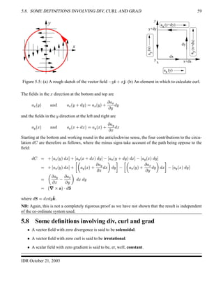
Lecture 5
Vector Operators: Grad, Div and Curl
In the first lecture of the second part of this course we move more to consider properties of fields. We
introduce three field operators which reveal interesting collective field properties, viz.
  the gradient of a scalar field,
  the divergence of a vector field, and
  the curl of a vector field.
There are two points to get over about each:
  The mechanics of taking the grad, div or curl, for which you will need to brush up your multivariate
calculus.
  The underlying physical meaning — that is, why they are worth bothering about.
In Lecture 6 we will look at combining these vector operators.
5.1 The gradient of a scalar field
Recall the discussion of temperature distribution throughout a room in the overview, where we wondered
how a scalar would vary as we moved off in an arbitrary direction. Here we find out how to.
If
¡£¢¥¤§¦©¨¦ is a scalar field, ie a scalar function of position  ¤§¦©¨¦  in 3 dimensions, then its
gradient at any point is defined in Cartesian co-ordinates by
!#©$ % ¡ 
 ¡
 ¤(')10
 ¡
 ¨1'230
 ¡
  '465
It is usual to define the vector operator
7  ')

 ¤ 0 '2

 ¨ 0 '4 
 
which is called “del” or “nabla”. Then
!#©$ % ¡98@7A¡
51
52 LECTURE 5. VECTOR OPERATORS: GRAD, DIV AND CURL
Note immediately that
7A¡ is a vector field!
Without thinking too carefully about it, we can see that the gradient tends to point in the direction of
greatest change of the scalar field. Later we will be more precise.
 
Worked examples of gradient evaluation
1.
¡  ¤¢¡
Only
¤£  ¤ exists so
7A¡ ¦¥
¤ ') 5
2.
¡ ¨§
¡
§
¡
 ¤¢¡ 0 ¨©¡ 0 ¡
, so
7A¡  ¥
¤ ') 0 ¥
¨ '2 0 ¥
 '4
 ¥ 5
3.
¡   , where  is constant.
7A¡ 

')

 ¤ 0 '2

 ¨ 0 '4 
 
¢! ¤ 0  ¡ ¨ 0 #   !
') 0  ¡ '2 0 $ '4 ¨
5
4.
¡ ¦%
¢ §

¡ %
¢¤ §¦©¨¦ ¦%
¢ §
¢¤ §¦©¨¦ 
Now #'
)(
102'
043
)3
$(
, #'
)5
106'
073
)3
)5
, and #'
$8
902'
043
)3
#8
, so
7A¡ 
 %
 ¤ ') 0
 %
 ¨ '2 0
 %
  '4 A@
%
@
§CB
 §
 ¤ ') 0
 §
 ¨ '2 0
 §
  '4ED
But § GF
¤ ¡ 0 ¨ ¡ 0  ¡
, so
 §
£  ¤  ¤ £
§ and similarly for
¨ ¦ . Hence
7A¡  @
%
@
§HB
 §
 ¤ ') 0
 §
 ¨ '2 0
 §
  '4 D
 @
%
@
§PI
¤ ') 0 ¨ '2 0  '4
§ Q
 @
%
@
§SR

§¤T
5
5.2. THE SIGNIFICANCE OF GRAD 53
grad 
¡£¢¥¤¦¡¨§  © ¡¢¤¦¡
¡¦§  © ¡
¤¦¡
Figure 5.1: The directional derivative
5.2 The significance of grad
We have seen that
7A¡ 
 ¡
 ¤ ') 0
 ¡
 ¨ '2 0
 ¡
  '4
so if we move a small amount
@
  @
¤ ') 0
@
¨ '2 0
@
 '4 the change in
¡ is (see figure 5.1)
@
¡ 
 ¡
 ¤ @
¤ 0
 ¡
 ¨ @
¨ 0
 ¡
  @
  7A¡ 
@
 5
Now divide by
@

@
¡
@
  7 ¡  @

@

5
But remember that 
@
  @
 , so
@
 £
@
 is a unit vector in the direction of
@
 .
So
  !#©$ % ¡ has the property that the rate of change of
¡ wrt distance in a particular direction ( '
) is the
projection of !# $ % ¡ onto that direction (or the component of ! ©$ % ¡ in that direction).
The quantity
@
¡ £
@
 is called a directional derivative. Note that in general it has a different value for
each direction, and so has no meaning until you specify the direction.
We could also say that
  At any point P, !#©$ % ¡ points in the direction of greatest change of
¡ at P, and has magnitude equal
to the rate of change of
¡ wrt distance in that direction.
Another nice property emerges if we think of a surface of constant
¡ – that is the locus
¢¤ §¦©¨¦ for
¡£¢¥¤§¦©¨¦  !$#%' $ #(
54 LECTURE 5. VECTOR OPERATORS: GRAD, DIV AND CURL
−4
−2
0
2
4
−4
−2
0
2
4
0
0.02
0.04
0.06
0.08
0.1
Figure 5.2:
If we move a tiny amount within the surface, that is in any tangential direction, there is no change in
¡ ,
so
@
¡ £
@
 ¡  . So for any
@
 £
@
 in the surface
7A¡  @

@
    5
This can only be satisfied if
  ! ©$ % ¡ is NORMAL to a surface of constant
¡ .
Surface of constant U
gradU
Surface of constant U
These are called Level Surfaces
Figure 5.3:
5.3 The divergence of a vector field
The divergence computes a scalar quantity from a vector field by differentiation.
5.4. THE SIGNIFICANCE OF  ¢¡¤£ 55
More precisely, if ¥ ¢¥¤§¦©¨¦ is a vector function of position in 3 dimensions, that is ¥ §¦ ')0 ¦ ¡ '2 0 ¦  '4 ,
then its divergence at any point is defined in Cartesian co-ordinates by
%©¨ ¥ 
 ¦ ¤ 0
 ¦ ¡
 ¨ 0
 ¦ 
 
We can write this in a simplified notation using a scalar product with the
7 vector differential operator:
%©¨ ¥ 

')

 ¤ 0 '2

 ¨ 0 '4 
   ¥  7 ¥
Notice that the divergence of a vector field is a scalar field.
 
Worked examples of divergence evaluation
¥ div¥¤ ') 
 ¢  ¤ ') 0 ¨ '2 0  '4  
3
   
§
¢   
 £
§ where  is constant
Let us show the third example.
The
¤ component of  £
§

is
¤ 5¢ ¥¤ ¡ 0 ¨ ¡ 0  ¡   ¡
, and we need to find
 £  ¤ of it.

 ¤ ¤ 5¢ ¥¤ ¡ 0 ¨ ¡ 0  ¡    ¡
  5¢ ¥¤ ¡ 0 ¨ ¡ 0  ¡    ¡ 0 ¤! 
¥
¢¥¤ ¡ 0 ¨ ¡ 0  ¡  #  ¡ 5¥
¤  §
 %$
  ¤ ¡
§
 ¡
Adding this to similar terms for
¨ and
 gives
§
  $   ¢¤ ¡ 0 ¨ ¡ 0  ¡  §
 ¡   §
 
¢' # ¡ 
5.4 The significance of (0)21
Consider a typical vector field, water flow, and denote it by ¥ ¢   . This vector has magnitude equal to the
mass of water crossing a unit area perpendicular to the direction of ¥ per unit time.
Now take an infinitesimal volume element
@#3 and figure out the balance of the flow of ¥ in and out of
@43 .
To be specific, consider the volume element
@43  @
¤
@
¨
@
 in Cartesian co-ordinates, and think first
about the face of area
@
¤
@
 perpendicular to the
¨ axis and facing outwards in the negative
¨ direction.
(That is, the one with surface area
@65  @
¤
@
 '2 .)
The component of the vector ¥ normal to this face is ¥  '2 7¦ 5
, and is pointing inwards, and so the its
contribution to the OUTWARD flux from this surface is
¥ 
@©5  ¦ 5
¢ ¨ 
@

@
¤ 5
(Flux here means mass per unit time.)
56 LECTURE 5. VECTOR OPERATORS: GRAD, DIV AND CURL
dS = -dxdz j
y
x
z
dz
dx
dy
jdS = +dxdz
Figure 5.4: Elemental volume for calculating divergence.
A similar contribution, but of opposite sign, will arise from the opposite face, but we must remember
that we have moved along
¨ by an amount
@
¨ , so that this OUTWARD amount is
¦ 5
¢¨ 0
@
¨ 
@

@
¤ 

¦ 5
0
 ¦ 5 ¨ @
¨ 
@
¤
@

The total outward amount from these two faces is
 ¦ 5 ¨ @
¨
@
¤
@
 
 ¦ 5 ¨ @#3
Summing the other faces gives a total outward flux of
  ¦ ( ¤ 0
 ¦ 5 ¨ 0
 ¦ 8  
@#3  7  ¥ @#3
Take home message: The divergence of a vector field represents the flux generation per unit volume at
each point of the field. (Divergence because it is an efflux not an influx.)
Interestingly we also saw that the total efflux from the infinitesimal volume was equal to the flux inte-
grated over the surface of the volume.
(NB: The above does not constitute a rigorous proof of the assertion because we have not proved that the
quantity calculated is independent of the co-ordinate system used, but it will suffice for our purposes.
5.5 The Laplacian: (0)21
¡£¢¥¤§¦
(©¨ of a scalar field
Recall that !# $ % ¡ of any scalar field
¡ is a vector field. Recall also that we can compute the divergence
of any vector field. So we can certainly compute %©¨ ¢ ! ©$ % ¡  , even if we don’t know what it means yet.
5.5. THE LAPLACIAN:  ¢¡¤£ ¢¡ £¢¥¤
  ¡  OF A SCALAR FIELD 57
Here is where the
7 operator starts to be really handy.
7 
¢ 7 ¡  

')

 ¤ 0 '2

 ¨ 0 '4 
   
 
')

 ¤ 0 '2

 ¨ 0 '4 
  
¡ 

 
')

 ¤ 0 '2

 ¨ 0 '4 
   

')

 ¤ 0 '2

 ¨ 0 '4 
   
¡

  ¡
 ¤ ¡ 0
 ¡
 ¨ ¡ 0
 ¡
  ¡ 
¡

  ¡ ¡
 ¤ ¡ 0
 ¡ ¡
 ¨ ¡ 0
 ¡ ¡
  ¡ 
This last expression occurs frequently in engineering science (you will meet it next in solving Laplace’s
Equation in partial differential equations). For this reason, the operator ¦
¡
is called the “Laplacian”
¦
¡ ¡ 
  ¡
 ¤ ¡ 0
 ¡
 ¨ ¡ 0
 ¡
  ¡ 
¡
Laplace’s equation itself is
¦
¡ ¡   
 
Examples of §©¨ evaluation
 § ¨ 

¨¨!#$¨%'(¨0) 1
 ¨ 32 456327'1(8 ¨ 
9A@  B
Let’s prove the last example (which is particularly significant – can you guess why?).
 £
§  ¢¥¤¢¡ 0 ¨©¡ 0 ¡   ' ¡
and so

 ¤

 ¤ ¢¥¤ ¡ 0 ¨ ¡ 0  ¡   ' ¡


 ¤ ¤ 5¢¤ ¡ 0 ¨ ¡ 0  ¡    ¡
 ¢¥¤ ¡ 0 ¨ ¡ 0  ¡    ¡ 0  ¤ 5¤ 5¢¤ ¡ 0 ¨ ¡ 0  ¡  #  ¡
 ¢  £
§
  ¢  0  ¤ ¡ £
§
¡ 
Adding up similar terms for
¨ and

¦
¡ 
§


§


 0  ¢¥¤¢¡ 0 ¨ ¡ 0 ¤¢¡ 
§
¡    
58 LECTURE 5. VECTOR OPERATORS: GRAD, DIV AND CURL
5.6 The curl of a vector field
So far we have seen the operator
7
  Applied to a scalar field
7 ¡ ; and
  Dotted with a vector field
7 ¥ .
You are now overwhelmed by that irrestible temptation to
  cross it with a vector field
7   ¥
This gives the curl of a vector field
7¡  ¥ 8 £¢ ¥¤¢ ¥ 
We can follow the pseudo-determinant recipe for vector products, so that
7¡  ¥ 
¦¦¦¦¦¦
') '2 '4

)(

)5

$8¦ (
¦ 5
¦ 8
¦¦¦¦¦¦

  ¦ 8 ¨
 ¦ 5   ') 0
  ¦ ( 
 ¦ 8 ¨  '2 0
  ¦ 5 ¤
 ¦ ( ¨  '4
 
Examples of curl evaluation
¥ 7§  ¥
¨ ') 0 ¤ '2 ¥ '4
¤¢¡¨©¡ '4 ¥
¤¢¡¨ ') ¥
¤ ¨©¡
'2
5.7 The signficance of curl
Perhaps the first example gives a clue. The field ¥  ¨ ') 0 ¤ '2 is sketched in Figure 5.5(a). (It is the
field you would calculate as the velocity field of an object rotating with ¨    ¦   ¦   .) This field has a
curl of ¥ '4 , which is in the r-h screw out of the page. You can also see that a field like this must give a
finite value to the line integral around the complete loop © ¥ 
@
 5
In fact curl is closely related to the line integral around a loop. The circulation of a vector ¥ round any
closed curve  is defined to be

 ¥ 
@

and the curl of the vector field ¥ represents the vorticity, or circulation per unit area, of the field.
Our proof uses the small rectangular element
@
¤ by
@
¨ shown in Figure 5.5(b). Consider the circulation
round the perimeter of a rectangular element.
5.8. SOME DEFINITIONS INVOLVING DIV, CURL AND GRAD 59
y
x
ax(y)
a(x)y
ax(y+dy)
ay(x+dx)
dx
dy
y
y
x x+dx
y+dy
Figure 5.5: (a) A rough sketch of the vector field
¨ ') 0 ¤ '2 . (b) An element in which to calculate curl.
The fields in the
¤ direction at the bottom and top are
¦ (
¢ ¨  $ # % ¦ (
¢¥¨ 0
@
¨   ¦ (
¢¥¨  0
 ¦ ( ¨ @
¨
and the fields in the
¨ direction at the left and right are
¦ 5
¢¤  $ # % ¦ 5
¢¤ 0
@
¤  §¦ 5
¢¤  0
 ¦ 5 ¤ @
¤
Starting at the bottom and working round in the anticlockwise sense, the four contributions to the circu-
lation
@
 are therefore as follows, where the minus signs take account of the path being oppose to the
field:
@
  0 ¦ (
¢ ¨ 
@
¤  0 ¦ 5
¢¥¤ 0
@
¤ 
@
¨  ¦ (
¢ ¨ 0
@
¨ 
@
¤  ¦ 5
¢¤ 
@
¨ 
 0 ¦ (
¢ ¨ 
@
¤  0
B

¦ 5
¢¤  0
 ¦ 5 ¤ @
¤ 
@
¨ D
B

¦ (
¢¥¨  0
 ¦ ( ¨ @
¨ 
@
¤ D
¦ 5
¢¤ 
@
¨ 

  ¦ 5 ¤
 ¦ ( ¨ 
@
¤
@
¨
 ¢ 7§  ¥  
@65
where
@65  @
¤
@
¨ '4 .
NB: Again, this is not a completely rigorous proof as we have not shown that the result is independent
of the co-ordinate system used.
5.8 Some definitions involving div, curl and grad
  A vector field with zero divergence is said to be solenoidal.
  A vector field with zero curl is said to be irrotational.
  A scalar field with zero gradient is said to be, er, well, constant.
IDR October 21, 2003
60 LECTURE 5. VECTOR OPERATORS: GRAD, DIV AND CURL
Lecture 6
Vector Operator Identities
In this lecture we look at more complicated identities involving vector operators. The main thing to
appreciate it that the operators behave both as vectors and as differential operators, so that the usual rules
of taking the derivative of, say, a product must be observed.
We shall derive these using both conventional grunt, and using the compact notation. Note that the
relevance of these identities may only become clear later in other Engineering courses.
6.1 Identity 1: curl grad ¨ =   ¡   ¨ ¢ £
7§  7A¡ 
¦¦¦¦¦¦
') '2 '4
¤£  ¤ ¤£  ¨ ¤£  
 ¡ £  ¤  ¡ £  ¨  ¡ £  
¦¦¦¦¦¦
 ')
  ¡ ¡
 ¨  
 ¡ ¡
   ¨  0 '2 ¢  0 '4 ¢ 
 ¤
5
Note that
7¡  7 can be thought of as a null operator.
6.2 Identity 2: div curl ¥ =   ¦§  ¡ ¥¨¢ ©
7 
7§  ¥ 
¦¦¦¦¦¦
 £  ¤ ¤£  ¨ ¤£  
 £  ¤ ¤£  ¨ ¤£  
¦ (
¦ 5
¦ 8
¦¦¦¦¦¦

 ¡
¦ 8 ¤  ¨
 ¡
¦ 5 ¤  
 ¡
¦ 8 ¨  ¤ 0
 ¡
¦ ( ¨  
 ¡
¦ 5   ¤
 ¡
¦ (   ¨
  
61
62 LECTURE 6. VECTOR OPERATOR IDENTITIES
6.3 Identity 3: div and curl of ¨ ¥
Suppose that
¡£¢   is a scalar field and that ¥ ¢   is a vector field and we are interested in the product
¡ ¥ ,
which is a vector field so we can compute its divergence and curl. For example the density ¡ ¢   of a fluid
is a scalar field, and the instantaneous velocity of the fluid ¢ ¢   is a vector field, and we are probably
interested in mass flow rates for which we will be interested in ¡ ¢   ¢ ¢   .
The divergence (a scalar) of the product
¡ ¥ is given by:
7 
¢ ¡ ¥   7 
¢ ¡ ¥ 
 ¡£¢ 7   ¥  0 ¢ 7 ¡  ¥
 ¡ %©¨  ¥ 0 ¢ !#©$ % ¡  ¥
In a similar way, we can take the curl of the vector field
¡ ¥ , and the result should be a vector field:
7¡  ¢ ¡ ¥   ¡ 7§  ¥ 0 ¢ 7A¡    ¥ 5
6.4 Identity 4: div of ¥ ¡
£
Life quickly gets trickier when vector or scalar products are involved: For example, it is not that obvious
that
%6¨ ¢ ¥  ¥¤   £¢ ¥¤¥ 
¤ ¥  £¢ ¥¤¤
To show this, use the determinant:
¦¦¦¦¦¦
 £  ¤§¦  £  ¤©¨ ¤£  ¤
¦ (
¦ 5
¦ 8
(

5

8
¦¦¦¦¦¦ 

 ¤ ¦ 5

8
¦ 8

5
 0

 ¨ ¦ 8

(
¦ (

8
 0

  ¦ (

5
¦ 5

(

 5 5 5 $ % ! ¢     ! % ¢%
5 5 5
 £¢ ¥¤¥ 
¤ ¥ 
¢ curl
¤ 
6.5 Vector operator identities in HLT
There is a kind of cottage industry in inventing vector identities. HLT contains a lot of them. So why not
leave it at that?
First, since !#©$ % , %©¨ and  ¢  ¤ describe key aspects of vectors fields, they arise often in practice, and
so the identities can save you a lot of time and hacking of partial derivatives, as we will see when we
consider Maxwell’s equation as an example later.
Secondly, they help to identify other practically important vector operators. We now look at such an
example.
6.6. IDENTITY 5:  ¢¡ ¢¤£ ¢¦¥  ¨§  63
6.6 Identity 5: ©
¤ ¡
¥ ¡
£

£¢ ¥¤¢ ¥  ¥¤  
¦¦¦¦¦¦
') '2 '4
¤£  ¤  £  ¨ ¤£  
¦ 5

8
¦ 8

5
¦ 8

(
¦ (

8
¦ (

5
¦ 5

(
¦¦¦¦¦¦
so the ') component is

 ¨ ¢ ¦ (

5
¦ 5

(
 
  ¢ ¦ 8

(
¦ (

8

which can be written as the sum of four terms:
¦ (
  
5 ¨ 0
 
8  D 
(
  ¦ 5 ¨ 0
 ¦ 8  D 0


5

 ¨ 0 
8

   ¦ (

¦ 5

 ¨ 0 ¦ 8


(
Adding ¦ ( 
)(
to the first of these, and subtracting from the last, and doing the same with

( 
)(
to the
other two terms, we find that:
7§  ¢ ¥   ¤   ¢ 7 
¤  ¥ ¢ 7 ¥  ¤ 0 ¤ 
76 ¥ ¥ 
7  ¤
where ¥ 
76 can be regarded as new, and very useful, scalar differential operator.
6.7 Definition of the operator ¥ ¦§  !
This is a scalar operator, but it can obviously can be applied to a scalar field, resulting in a scalar field,
or to a vector field resulting in a vector field:
¥ 
7  8
B
¦ (

 ¤ 0 ¦ 5

 ¨ 0 ¦ 8

  D 5
6.8 Identity 6: ©
¤ ¡
©
¤
¥  for you to derive
The following important identity is stated, and let as an exercise:
£¢ ¥¤¢ £¢ ¥¤¥   ! ©$ % %©¨ ¥ ¦
¡
¥
where
¦
¡
¥  ¦
¡
¦ (
') 0 ¦
¡
¦ 5
'2 0 ¦
¡
¦ 8
'4
 
Example of Identity 6: electromagnetic waves
Background: Maxwell established a set of four vector equations which are fundamental to working out
how eletromagnetic waves propagate. The entire telecommunications industry is built on these!
%©¨$#  ¡
%©¨ §   
£¢  ¤% 

(' §
£¢ ¥¤0)  1 0

(' #
64 LECTURE 6. VECTOR OPERATOR IDENTITIES
In addition, we can assume the following
§ ¡  3
 £¢ ) , 1 ¥¤ % , # ¡¦ 3
¦§¢ % ,
where all the scalars are constants.
Question: Show that in a material with no free charge, ¡    , and with zero conductivity, ¤    , the
eletric field % must be a solution of the wave equation
¦
¡ % ¡  3
 £¢¨¦ 3
¦§¢ ¢  ¡ % £ (' ¡  5
Answer: The good news is that we can do this knowing little about EM waves!
%6¨$#  %©¨  ¢ ¦ 3
¦§¢ %  ©¦ 3
¦¢ %©¨ %  ¡   %©¨  §  %©¨  ¢   3
 £¢ )  ¥  3
 £¢ %6¨$)   
£¢ ¥¤%   § £ ('
   3
 £¢ ¢ ) £ (' 
 ¢  ¤)  1 0  # £ ('
 ¤ 0 ¦ 3
¦§¢ ¢  % £ (' 
But we know (or rather you worked out) that £¢  ¤£¢ ¥¤0%  !# $ % %©¨ $% ¦
¡ % , so
 ¢  ¤£¢  ¤0%   ¢  ¤    3
 ¢ ¢  ) £ ('    !#©$ % %©¨ (% ¦
¡ %
so interchanging the order of partial differentation, and using %©¨ $%    :
  3
 £¢

('  ¢  ¤0)   ¦
¡ %
  3
 £¢

('
B
¦ 3
¦§¢
 %
(' D
 ¦
¡ %
  3
 £¢¨¦ 3
¦§¢
 ¡ %
(' ¡  ¦
¡ %
6.9 Grad, div, curl and
 ¥ in curvilinear co-ordinate systems
It is possible to obtain general expressions for grad, div and curl in any orthogonal curvilinear co-ordinate
system by making use of the  factors which were introduced in Lecture 4.
We recall that the unit vector in the direction of increasing  , with  and  being kept constant, is


where  is the radius vector, and
  
¦¦¦¦
  
¦¦¦¦
and similar expressions apply for the other co-ordinate directions. Then
@
 ©  
@
 0  ! ¢ @
 0   #
@
 5
6.10. GRAD IN CURVILINEAR COORDINATES 65
6.10 Grad in curvilinear coordinates
Using the properties of the gradient of a scalar field obtained previously,
7A¡ 
@
  @
¡ 
 ¡
  @
 0
 ¡
 @
 0
 ¡
  @

It follows that
7A¡ 
¢   
@
 0  ! ¢ @
 0   #
@
  
 ¡
  @
 0
 ¡
  @
 0
 ¡
  @

The only way this can be satisfied for independent
@
 ,
@
 ,
@
 is when
7A¡ 

 
 ¡
  ' 0 
 !
 ¡
  '¢ 0 
 
 ¡
  '#
6.11 Divergence in curvilinear coordinates
Expressions can be obtained for the divergence of a vector field in orthogonal curvilinear co-ordinates
by making use of the flux property.
We consider an element of volume
@#3 . Although earlier we derived this as the volume of a parallelop-
iped, and found that the
@#3 
¦¦¦¦
 ¢¥¤§¦©¨¦
 ¢  ¦  ¦  
¦¦¦¦ @
 @
 @

If the curvilinear coordinates are orthogonal then the little volume is a cuboid (to first order in small
quantities) and
@#3 ¡   !   @
 @
 @
 5
However, it is not quite a cuboid: the area of two opposite faces will differ as the scale parameters are
functions of  ,  and  in general.
So the net efflux from the two faces in the '¢ direction shown in Figure 6.1 is
 B
¦ ! 0
 ¦ !  @
 D
B
  0
    @
 D
B
  0
    @
 D
@
 @
 ¦ !     @
 @


 ¢ ¦ !     
  @
 @
 @

which is easily shown by multiplying the first line out and dropping second order terms (i.e.
¢
@
 $¡
).
By definition div is the net efflux per unit volume, so summing up the other faces:
%©¨  ¥ @#3 
  ¢ ¦   !   
 
0
 ¢ ¦ !     
 
0
 ¢ ¦     ! 
  
@
 @
 @

¡
%6¨ ¥    !   @
 @
 @
 
  ¢ ¦   !   
 
0
 ¢ ¦ !     
 
0
 ¢ ¦     ! 
  
@
 @
 @
66 LECTURE 6. VECTOR OPERATOR IDENTITIES
w
u
y
The scale params are
h (v) dw
h (v+dv) dw
h (v+dv) du
h (v) du
u
w
w
u
h dvv
functions of u,v,w
Figure 6.1: Elemental volume for calculating divergence in orthogonal curvilinear coordinates
So, finally,
%6¨ ¥ 

   !  
  ¢ ¦   !   
 
0
 ¢ ¦ !     
 
0
 ¢ ¦     ! 
  
6.12 Curl in curvilinear coordinates
Recall from Lecture 5 that we computed the
 component of curl as the circulation per unit area — the
contents of the brackets
¢  in the expression for the element of circulation
@
 
  ¦ 5 ¤
 ¦ ( ¨ 
@
¤
@
¨
By analogy with our derivation of divergence, you will realize that for an orthogonal curvilinear coordi-
nate system we can write the area as    ! @
 @
 . But the opposite sides are no longer quite of the same
length. The lower of the pair in Figure 6.2 is length   ¢  
@
 , but the upper is of length   ¢  0
@
 
@

Summing this pair gives a contribution to the circulation
¦  ¢     ¢  
@
 ¦  ¢  0
@
    ¢  0
@
 
@
 
 ¢   ¦  
  @
 @

and together with the other pair:
@
 
  ¢   ¦  
 
0
 ¢  ! ¦ ! 
  
@
 @

So the circulation per unit area is
@

   ! @
 @
 

   !
  ¢  ! ¦ ! 
 
 ¢   ¦
6.13. THE LAPLACIAN IN CURVILINEAR COORDINATES 67
y
y
a
a
u
u u+du
u
u
u
v+dv
(v+dv)
h (v+dv) du
dv
(v)
h (v) du
Figure 6.2: Elemental loop for calculating curl in orthogonal curvilinear coordinates
and hence curl is
£¢ ¥¤¥ ¢  ¦  ¦   

 !  
  ¢   ¦  
 
 ¢  ! ¦ ! 
   ' 0 
   
  ¢   ¦  
 
 ¢   ¦  
   '¢ 0

   !
  ¢  ! ¦ ! 
 
 ¢   ¦  
   '#
6.13 The Laplacian in curvilinear coordinates
Substitution of the components of !#©$ % ¡ into the expression for %©¨ ¥ immediately (!*?) gives the
following expression for the Laplacian in general orthogonal co-ordinates:
¦
¡ ¡ 

   !   B


 !  
 
 ¡
   0


 !
 ¡
   0


   !
 
 ¡
  
D 5
6.14 Grad, etc, in cylindrical polars
We recall that   §  ! %¡  ') 0 §% ¨ #¢  '2 0  '4 , and that   
  £   , and so
  F
¢  !$%
¡
  0 ¤£¦¥ ¡
 
   ¦
 ¡ 
§
¢ §
¡
% ¨ #
¡
  0 §
¡
 ! %
¡
 
  §
¦
68 LECTURE 6. VECTOR OPERATOR IDENTITIES
Hence
! ©$ % ¡ 
 ¡
 §
' 
3
0 
§
 ¡
  
' ¢¡ 0
 ¡
  '4
%©¨  ¥ 

§
  ¢ § ¦ 3

 §
0
 ¦ ¡
  
 0
 ¦ 8 
£¢ ¥¤¥ 
 
§
 ¦ 8  
 ¦ ¡
   ' 
3
0
  ¦ 3 
 ¦ 8 §
 ' ¢¡ 0 
§
  ¢ § ¦ ¡ 
 §
 ¦ 3  
 '4
The derivation of the expression for ¦
¡ ¡ in cylindrical polar co-ordinates is set as a tutorial exercise.
6.15 Grad, etc, in spherical polars
We recall that  ¨§% ¨ #¤£ !$%¡  ') 0 § % ¨ #¤£ % ¨ #   '2 0 § !$%¥£ '4 so that
 
§
¢ % ¨ #
¡
£
¢  ! %
¡
  0 % ¨ #
¡
 
 0  !$%
¡
£
  
 ¡ 
§
¢ §
¡
 ! %
¡
£
¢ !$%
¡
  0 % ¨ #
¡
 
 0 §
¡
% ¨ #
¡
£
  §
 

§
¢ §
¡
% ¨ #
¡
£
¢ % ¨ #
¡
  0  !$%
¡
 
 ¨§ % ¨ #¤£
Hence
! ©$ % ¡ 
 ¡
 §
' 
3
0 
§
 ¡
 £
' ¢¦ 0 
§ % ¨ #§£
 ¡
  
' ¨¡
%©¨  ¥ 

§
¡
 ¢ §
¡
¦ 3

 §
0 
§ % ¨ #§£
 ¢ ¦ ¦ % ¨ #§£

 £
0 
§ % ¨ #§£
 ¦ ¡
  
£¢ ¥¤¥  ' 
3
§ % ¨ #§£
 
 £
¢ ¦ ¡ % ¨ #§£
 
  
¢ ¦ ¦   0 ' ¢¦
§% ¨ #¤£
 
  
¢ ¦ 3
 
 §
¢ ¦ ¡ § % ¨ #¤£
  0
' ¢¡
§
 
 §
¢ ¦ ¦ §
 
 £
¢ ¦ 3
 
  The derivation of the expression for ¦
¡ ¡ is set as a tutorial exercise.
 
Examples
Q1 Find  ¢  ¤¥ in (i) Cartesians and (ii) Spherical poplars when ¥  ¤ ¢¥¤ ') 0 ¨ '2 0  '4  .
6.15. GRAD, ETC, IN SPHERICAL POLARS 69
A1 (i) In Cartesians, using the pseudo determinant gives  ¢  ¤¥   '2 0 ¨ '4 .
(ii) By inspection, in spherical polars
¥  § % ¨ #¤£  ! %¡ 
¢ § ' 
3

so
¦ 3
¨§
¡
% ¨ #¤£ !$%¡ ¡  ¦ ¦ ¡ ¢  ¦ ¡    5
Hence
£¢  ¤¥  ' ¨¦
§% ¨ #¤£
 
  
¢ §
¡
% ¨ #¤£ !$%¡ 
  0
' ¢¡
§
 
 £
¢ §
¡
% ¨ #§£ !$%  
 
 ' ¨¦
§% ¨ #¤£
¢ §
¡
% ¨ #§£ % ¨ #  
 0 ' ¢¡
§
$
§
¡
 !$% £ !$%  
 
 ' ¢¦ ¢ §% ¨ #¢ 
 0 ' ¢¡ ¢ §  !$%¥£ !$%¡ 

Now, these two results should be the same, but to check we need expressions for ' 
3
etc in terms of
') etc.
Remember that we can work out the unit vectors ' 
3
and so on in terms of ') etc using
' 
3


@
§
  ' ¢¦ 

 ¡
 
@
£
  ' ¢¡ 


@
 
£      ¤ ') 0 ¨ '2 0  '4 5
Grinding through we find
¤¥
' 
3
' ¢¦
' ¢¡
¦§

¤¥
% ¨ #§£ !$%   % ¨ #§£ % ¨ #¢  !$%¥£
 !$%¥£ !$%¡   !$%¥£ % ¨ #   % ¨ #¤£
% ¨ #¢   !$%    
¦§¨¤¥
')
'2
'4
¦§
 ©

¤¥
')
'2
'4
¦§
Don’t be shocked to see a rotation matrix ©
 : we are after all rotating one right-handed orthogonal
coord system into another.
So the result in spherical polars is
£¢  ¤¥  ¢  !$%¥£ !$%¡  ') 0 !$%¥£ % ¨ #   '2 % ¨ #¤£ '4  ¢ § % ¨ #  
 0 ¢ % ¨ #   ') 0  !$%¡  '2  ¢ §  !$%¥£ !$%¡ 

 §  ! %¥£ '2 0 §% ¨ #§£ % ¨ #¢  '4
  '2 0 ¨ '4
which is exactly the result in Cartesians.
Q2 Find the divergence of the vector field ¥  §  where  is a constant vector (i) using Cartesian
coordinates and (ii) using Spherical Polar coordinates.
70 LECTURE 6. VECTOR OPERATOR IDENTITIES
A2 (i) Using Cartesian coords:
%©¨ ¥ 

 ¤ ¢¤ ¡ 0 ¨ ¡ 0  ¡  ' ¡ 
(
0 5 5 5
 ¤ 5¢¤ ¡ 0 ¨ ¡ 0  ¡   ' ¡ 
(
0 5 5 5


§
  
5
(ii) Using Spherical polars
¥  ¦ 3
' 
3
0 ¦ ¦ ' ¢¦ 0 ¦ ¡ ' ¢¡
and our first task is to find ¦ 3
and so on. We can’t do this by inspection, and finding their values
requires more work than you might think! Recall
¤¥
' 
3
' ¢¦
'  ¡
¦§

¤¥
% ¨ #§£  ! %   % ¨ #§£ % ¨ #¢  !$% £
!$%¥£  !$%¡  !$%¥£ % ¨ #   % ¨ #¤£
% ¨ #¢  !$%    
¦§ ¤¥
')
'2
'4
¦§
 ©

¤¥
')
'2
'4
¦§
Now the point is the same point in space whatever the coordinate system, so
¦ 3
' 
3
0 ¦ ¦ ' ¢¦ 0 ¦ ¡ ' ¢¡  ¦ (
') 0 ¦ 5
'2 0 ¦ 8
'4
and using the inner product
¤¥
¦ 3
¦ ¦
¦ ¡
¦§ ¡
¤¥
' 
3
' ¨¦
' ¢¡
¦§

¤¥
¦ (
¦ 5
¦ 8
¦§ ¡
¤¥
')
'2
'4
¦§
¤¥
¦ 3
¦ ¦
¦ ¡
¦§ ¡
©

¤¥
')
'2
'4
¦§

¤¥
¦ (
¦ 5
¦ 8
¦§ ¡
¤¥
')
'2
'4
¦§
¡
¤¥
¦ 3
¦ ¦
¦ ¡
¦§ ¡
©
 
¤¥
¦ (
¦ 5
¦ 8
¦§ ¡
¡
¤¥
¦ 3
¦ ¦
¦ ¡
¦§ ¡

¤¥
¦ (
¦ 5
¦ 8
¦§ ¡
©
 ¡
¡
¤¥
¦ 3
¦ ¦
¦ ¡
¦§
 ©

¤¥
¦ (
¦ 5
¦ 8
¦§
For our particular problem, ¦ (
 §

(
, etc, where

(
is a constant, so now we can write down
¦ 3
 §
¢ % ¨ #¤£  !$%¡ 

(
0 % ¨ #¤£ % ¨ #  

5
0 !$%¥£

8

¦ ¦  §
¢  !$%¥£ !$%  

(
0  ! %¥£ % ¨ #  

5
% ¨ #§£

8

¦ ¡  §
¢ % ¨ #  

(
0  !$%¡ 

5
6.15. GRAD, ETC, IN SPHERICAL POLARS 71
Now all we need to do is to bash out
%©¨  ¥ 

§
¡
 ¢ §
¡
¦ 3

 §
0 
§% ¨ #¤£
 ¢ ¦ ¦ % ¨ #¤£

 £
0 
§ % ¨ #¤£
 ¦ ¡
  
In glorious detail this is
%©¨  ¥   ¢ % ¨ #§£  ! %¡ 

(
0 % ¨ #¤£ % ¨ #  

5
0 !$% £

8
 0

% ¨ #§£
$
 !$%
¡
£ % ¨ #
¡
£
 ¢  !$%  

(
0 % ¨ #¢ 

5
 ¥ % ¨ # £  !$%¥£

8
 0

% ¨ #§£
¢  !$%  

(
% ¨ #  

5

A bit more bashing and you’ll find
%©¨  ¥  % ¨ #§£  !$%  

(
0 % ¨ #§£ % ¨ #¢ 

5
0  !$%¥£

8
 ' 
3
 
This is EXACTLY what you worked out before of course.
Take home messages from these examples:
All the trig was a bit tedious, but there are three important points!
  Just as physical vectors are independent of their coordinate systems, so are differential operators.
  Don’t forget about the vector geometry you did in the 1st year. Rotation matrices are useful!
  Spherical polars were NOT a good coordinate system in which to think about this problem. Let
the symmetry guide you.
IDR October 21, 2003

Graddivcurl1

  • 1.
    Lecture 5 Vector Operators:Grad, Div and Curl In the first lecture of the second part of this course we move more to consider properties of fields. We introduce three field operators which reveal interesting collective field properties, viz.   the gradient of a scalar field,   the divergence of a vector field, and   the curl of a vector field. There are two points to get over about each:   The mechanics of taking the grad, div or curl, for which you will need to brush up your multivariate calculus.   The underlying physical meaning — that is, why they are worth bothering about. In Lecture 6 we will look at combining these vector operators. 5.1 The gradient of a scalar field Recall the discussion of temperature distribution throughout a room in the overview, where we wondered how a scalar would vary as we moved off in an arbitrary direction. Here we find out how to. If ¡£¢¥¤§¦©¨¦ is a scalar field, ie a scalar function of position ¤§¦©¨¦ in 3 dimensions, then its gradient at any point is defined in Cartesian co-ordinates by !#©$ % ¡ ¡ ¤(')10 ¡ ¨1'230 ¡ '465 It is usual to define the vector operator 7 ') ¤ 0 '2 ¨ 0 '4 which is called “del” or “nabla”. Then !#©$ % ¡98@7A¡ 51
  • 2.
    52 LECTURE 5.VECTOR OPERATORS: GRAD, DIV AND CURL Note immediately that 7A¡ is a vector field! Without thinking too carefully about it, we can see that the gradient tends to point in the direction of greatest change of the scalar field. Later we will be more precise.   Worked examples of gradient evaluation 1. ¡ ¤¢¡ Only ¤£ ¤ exists so 7A¡ ¦¥ ¤ ') 5 2. ¡ ¨§ ¡ § ¡ ¤¢¡ 0 ¨©¡ 0 ¡ , so 7A¡ ¥ ¤ ') 0 ¥ ¨ '2 0 ¥ '4 ¥ 5 3. ¡ , where is constant. 7A¡ ') ¤ 0 '2 ¨ 0 '4 ¢! ¤ 0 ¡ ¨ 0 # ! ') 0 ¡ '2 0 $ '4 ¨ 5 4. ¡ ¦% ¢ § ¡ % ¢¤ §¦©¨¦ ¦% ¢ § ¢¤ §¦©¨¦ Now #' )( 102' 043 )3 $( , #' )5 106' 073 )3 )5 , and #' $8 902' 043 )3 #8 , so 7A¡ % ¤ ') 0 % ¨ '2 0 % '4 A@ % @ §CB § ¤ ') 0 § ¨ '2 0 § '4ED But § GF ¤ ¡ 0 ¨ ¡ 0 ¡ , so § £ ¤ ¤ £ § and similarly for ¨ ¦ . Hence 7A¡ @ % @ §HB § ¤ ') 0 § ¨ '2 0 § '4 D @ % @ §PI ¤ ') 0 ¨ '2 0 '4 § Q @ % @ §SR §¤T 5
  • 3.
    5.2. THE SIGNIFICANCEOF GRAD 53 grad  ¡£¢¥¤¦¡¨§  © ¡¢¤¦¡ ¡¦§  © ¡ ¤¦¡ Figure 5.1: The directional derivative 5.2 The significance of grad We have seen that 7A¡ ¡ ¤ ') 0 ¡ ¨ '2 0 ¡ '4 so if we move a small amount @ @ ¤ ') 0 @ ¨ '2 0 @ '4 the change in ¡ is (see figure 5.1) @ ¡ ¡ ¤ @ ¤ 0 ¡ ¨ @ ¨ 0 ¡ @ 7A¡ @ 5 Now divide by @ @ ¡ @ 7 ¡ @ @ 5 But remember that @ @ , so @ £ @ is a unit vector in the direction of @ . So   !#©$ % ¡ has the property that the rate of change of ¡ wrt distance in a particular direction ( ' ) is the projection of !# $ % ¡ onto that direction (or the component of ! ©$ % ¡ in that direction). The quantity @ ¡ £ @ is called a directional derivative. Note that in general it has a different value for each direction, and so has no meaning until you specify the direction. We could also say that   At any point P, !#©$ % ¡ points in the direction of greatest change of ¡ at P, and has magnitude equal to the rate of change of ¡ wrt distance in that direction. Another nice property emerges if we think of a surface of constant ¡ – that is the locus ¢¤ §¦©¨¦ for ¡£¢¥¤§¦©¨¦ !$#%' $ #(
  • 4.
    54 LECTURE 5.VECTOR OPERATORS: GRAD, DIV AND CURL −4 −2 0 2 4 −4 −2 0 2 4 0 0.02 0.04 0.06 0.08 0.1 Figure 5.2: If we move a tiny amount within the surface, that is in any tangential direction, there is no change in ¡ , so @ ¡ £ @ ¡  . So for any @ £ @ in the surface 7A¡ @ @   5 This can only be satisfied if   ! ©$ % ¡ is NORMAL to a surface of constant ¡ . Surface of constant U gradU Surface of constant U These are called Level Surfaces Figure 5.3: 5.3 The divergence of a vector field The divergence computes a scalar quantity from a vector field by differentiation.
  • 5.
    5.4. THE SIGNIFICANCEOF  ¢¡¤£ 55 More precisely, if ¥ ¢¥¤§¦©¨¦ is a vector function of position in 3 dimensions, that is ¥ §¦ ')0 ¦ ¡ '2 0 ¦ '4 , then its divergence at any point is defined in Cartesian co-ordinates by %©¨ ¥ ¦ ¤ 0 ¦ ¡ ¨ 0 ¦ We can write this in a simplified notation using a scalar product with the 7 vector differential operator: %©¨ ¥ ') ¤ 0 '2 ¨ 0 '4 ¥ 7 ¥ Notice that the divergence of a vector field is a scalar field.   Worked examples of divergence evaluation ¥ div¥¤ ') ¢ ¤ ') 0 ¨ '2 0 '4 3   § ¢ £ § where is constant Let us show the third example. The ¤ component of £ § is ¤ 5¢ ¥¤ ¡ 0 ¨ ¡ 0 ¡ ¡ , and we need to find £ ¤ of it. ¤ ¤ 5¢ ¥¤ ¡ 0 ¨ ¡ 0 ¡ ¡ 5¢ ¥¤ ¡ 0 ¨ ¡ 0 ¡ ¡ 0 ¤! ¥ ¢¥¤ ¡ 0 ¨ ¡ 0 ¡ # ¡ 5¥ ¤ § %$ ¤ ¡ § ¡ Adding this to similar terms for ¨ and gives § $ ¢¤ ¡ 0 ¨ ¡ 0 ¡ § ¡ § ¢' # ¡  5.4 The significance of (0)21 Consider a typical vector field, water flow, and denote it by ¥ ¢ . This vector has magnitude equal to the mass of water crossing a unit area perpendicular to the direction of ¥ per unit time. Now take an infinitesimal volume element @#3 and figure out the balance of the flow of ¥ in and out of @43 . To be specific, consider the volume element @43 @ ¤ @ ¨ @ in Cartesian co-ordinates, and think first about the face of area @ ¤ @ perpendicular to the ¨ axis and facing outwards in the negative ¨ direction. (That is, the one with surface area @65 @ ¤ @ '2 .) The component of the vector ¥ normal to this face is ¥ '2 7¦ 5 , and is pointing inwards, and so the its contribution to the OUTWARD flux from this surface is ¥ @©5 ¦ 5 ¢ ¨ @ @ ¤ 5 (Flux here means mass per unit time.)
  • 6.
    56 LECTURE 5.VECTOR OPERATORS: GRAD, DIV AND CURL dS = -dxdz j y x z dz dx dy jdS = +dxdz Figure 5.4: Elemental volume for calculating divergence. A similar contribution, but of opposite sign, will arise from the opposite face, but we must remember that we have moved along ¨ by an amount @ ¨ , so that this OUTWARD amount is ¦ 5 ¢¨ 0 @ ¨ @ @ ¤ ¦ 5 0 ¦ 5 ¨ @ ¨ @ ¤ @ The total outward amount from these two faces is ¦ 5 ¨ @ ¨ @ ¤ @ ¦ 5 ¨ @#3 Summing the other faces gives a total outward flux of ¦ ( ¤ 0 ¦ 5 ¨ 0 ¦ 8 @#3 7 ¥ @#3 Take home message: The divergence of a vector field represents the flux generation per unit volume at each point of the field. (Divergence because it is an efflux not an influx.) Interestingly we also saw that the total efflux from the infinitesimal volume was equal to the flux inte- grated over the surface of the volume. (NB: The above does not constitute a rigorous proof of the assertion because we have not proved that the quantity calculated is independent of the co-ordinate system used, but it will suffice for our purposes. 5.5 The Laplacian: (0)21 ¡£¢¥¤§¦ (©¨ of a scalar field Recall that !# $ % ¡ of any scalar field ¡ is a vector field. Recall also that we can compute the divergence of any vector field. So we can certainly compute %©¨ ¢ ! ©$ % ¡ , even if we don’t know what it means yet.
  • 7.
    5.5. THE LAPLACIAN: ¢¡¤£ ¢¡ £¢¥¤   ¡ OF A SCALAR FIELD 57 Here is where the 7 operator starts to be really handy. 7 ¢ 7 ¡ ') ¤ 0 '2 ¨ 0 '4 ') ¤ 0 '2 ¨ 0 '4 ¡ ') ¤ 0 '2 ¨ 0 '4 ') ¤ 0 '2 ¨ 0 '4 ¡ ¡ ¤ ¡ 0 ¡ ¨ ¡ 0 ¡ ¡ ¡ ¡ ¡ ¤ ¡ 0 ¡ ¡ ¨ ¡ 0 ¡ ¡ ¡ This last expression occurs frequently in engineering science (you will meet it next in solving Laplace’s Equation in partial differential equations). For this reason, the operator ¦ ¡ is called the “Laplacian” ¦ ¡ ¡ ¡ ¤ ¡ 0 ¡ ¨ ¡ 0 ¡ ¡ ¡ Laplace’s equation itself is ¦ ¡ ¡     Examples of §©¨ evaluation § ¨ ¨¨!#$¨%'(¨0) 1 ¨ 32 456327'1(8 ¨ 9A@ B Let’s prove the last example (which is particularly significant – can you guess why?). £ § ¢¥¤¢¡ 0 ¨©¡ 0 ¡ ' ¡ and so ¤ ¤ ¢¥¤ ¡ 0 ¨ ¡ 0 ¡ ' ¡ ¤ ¤ 5¢¤ ¡ 0 ¨ ¡ 0 ¡ ¡ ¢¥¤ ¡ 0 ¨ ¡ 0 ¡ ¡ 0 ¤ 5¤ 5¢¤ ¡ 0 ¨ ¡ 0 ¡ # ¡ ¢ £ § ¢ 0 ¤ ¡ £ § ¡ Adding up similar terms for ¨ and ¦ ¡ § § 0 ¢¥¤¢¡ 0 ¨ ¡ 0 ¤¢¡ § ¡  
  • 8.
    58 LECTURE 5.VECTOR OPERATORS: GRAD, DIV AND CURL 5.6 The curl of a vector field So far we have seen the operator 7   Applied to a scalar field 7 ¡ ; and   Dotted with a vector field 7 ¥ . You are now overwhelmed by that irrestible temptation to   cross it with a vector field 7   ¥ This gives the curl of a vector field 7¡  ¥ 8 £¢ ¥¤¢ ¥ We can follow the pseudo-determinant recipe for vector products, so that 7¡  ¥ ¦¦¦¦¦¦ ') '2 '4 )( )5 $8¦ ( ¦ 5 ¦ 8 ¦¦¦¦¦¦ ¦ 8 ¨ ¦ 5 ') 0 ¦ ( ¦ 8 ¨ '2 0 ¦ 5 ¤ ¦ ( ¨ '4   Examples of curl evaluation ¥ 7§  ¥ ¨ ') 0 ¤ '2 ¥ '4 ¤¢¡¨©¡ '4 ¥ ¤¢¡¨ ') ¥ ¤ ¨©¡ '2 5.7 The signficance of curl Perhaps the first example gives a clue. The field ¥ ¨ ') 0 ¤ '2 is sketched in Figure 5.5(a). (It is the field you would calculate as the velocity field of an object rotating with ¨   ¦   ¦ .) This field has a curl of ¥ '4 , which is in the r-h screw out of the page. You can also see that a field like this must give a finite value to the line integral around the complete loop © ¥ @ 5 In fact curl is closely related to the line integral around a loop. The circulation of a vector ¥ round any closed curve is defined to be ¥ @ and the curl of the vector field ¥ represents the vorticity, or circulation per unit area, of the field. Our proof uses the small rectangular element @ ¤ by @ ¨ shown in Figure 5.5(b). Consider the circulation round the perimeter of a rectangular element.
  • 9.
    5.8. SOME DEFINITIONSINVOLVING DIV, CURL AND GRAD 59 y x ax(y) a(x)y ax(y+dy) ay(x+dx) dx dy y y x x+dx y+dy Figure 5.5: (a) A rough sketch of the vector field ¨ ') 0 ¤ '2 . (b) An element in which to calculate curl. The fields in the ¤ direction at the bottom and top are ¦ ( ¢ ¨ $ # % ¦ ( ¢¥¨ 0 @ ¨ ¦ ( ¢¥¨ 0 ¦ ( ¨ @ ¨ and the fields in the ¨ direction at the left and right are ¦ 5 ¢¤ $ # % ¦ 5 ¢¤ 0 @ ¤ §¦ 5 ¢¤ 0 ¦ 5 ¤ @ ¤ Starting at the bottom and working round in the anticlockwise sense, the four contributions to the circu- lation @ are therefore as follows, where the minus signs take account of the path being oppose to the field: @ 0 ¦ ( ¢ ¨ @ ¤ 0 ¦ 5 ¢¥¤ 0 @ ¤ @ ¨ ¦ ( ¢ ¨ 0 @ ¨ @ ¤ ¦ 5 ¢¤ @ ¨ 0 ¦ ( ¢ ¨ @ ¤ 0 B ¦ 5 ¢¤ 0 ¦ 5 ¤ @ ¤ @ ¨ D B ¦ ( ¢¥¨ 0 ¦ ( ¨ @ ¨ @ ¤ D ¦ 5 ¢¤ @ ¨ ¦ 5 ¤ ¦ ( ¨ @ ¤ @ ¨ ¢ 7§  ¥ @65 where @65 @ ¤ @ ¨ '4 . NB: Again, this is not a completely rigorous proof as we have not shown that the result is independent of the co-ordinate system used. 5.8 Some definitions involving div, curl and grad   A vector field with zero divergence is said to be solenoidal.   A vector field with zero curl is said to be irrotational.   A scalar field with zero gradient is said to be, er, well, constant. IDR October 21, 2003
  • 10.
    60 LECTURE 5.VECTOR OPERATORS: GRAD, DIV AND CURL
  • 11.
    Lecture 6 Vector OperatorIdentities In this lecture we look at more complicated identities involving vector operators. The main thing to appreciate it that the operators behave both as vectors and as differential operators, so that the usual rules of taking the derivative of, say, a product must be observed. We shall derive these using both conventional grunt, and using the compact notation. Note that the relevance of these identities may only become clear later in other Engineering courses. 6.1 Identity 1: curl grad ¨ =   ¡   ¨ ¢ £ 7§  7A¡ ¦¦¦¦¦¦ ') '2 '4 ¤£ ¤ ¤£ ¨ ¤£ ¡ £ ¤ ¡ £ ¨ ¡ £ ¦¦¦¦¦¦ ') ¡ ¡ ¨ ¡ ¡ ¨ 0 '2 ¢ 0 '4 ¢ ¤ 5 Note that 7¡  7 can be thought of as a null operator. 6.2 Identity 2: div curl ¥ =   ¦§  ¡ ¥¨¢ © 7 7§  ¥ ¦¦¦¦¦¦ £ ¤ ¤£ ¨ ¤£ £ ¤ ¤£ ¨ ¤£ ¦ ( ¦ 5 ¦ 8 ¦¦¦¦¦¦ ¡ ¦ 8 ¤ ¨ ¡ ¦ 5 ¤ ¡ ¦ 8 ¨ ¤ 0 ¡ ¦ ( ¨ ¡ ¦ 5 ¤ ¡ ¦ ( ¨   61
  • 12.
    62 LECTURE 6.VECTOR OPERATOR IDENTITIES 6.3 Identity 3: div and curl of ¨ ¥ Suppose that ¡£¢ is a scalar field and that ¥ ¢ is a vector field and we are interested in the product ¡ ¥ , which is a vector field so we can compute its divergence and curl. For example the density ¡ ¢ of a fluid is a scalar field, and the instantaneous velocity of the fluid ¢ ¢ is a vector field, and we are probably interested in mass flow rates for which we will be interested in ¡ ¢ ¢ ¢ . The divergence (a scalar) of the product ¡ ¥ is given by: 7 ¢ ¡ ¥ 7 ¢ ¡ ¥ ¡£¢ 7 ¥ 0 ¢ 7 ¡ ¥ ¡ %©¨ ¥ 0 ¢ !#©$ % ¡ ¥ In a similar way, we can take the curl of the vector field ¡ ¥ , and the result should be a vector field: 7¡  ¢ ¡ ¥ ¡ 7§  ¥ 0 ¢ 7A¡   ¥ 5 6.4 Identity 4: div of ¥ ¡ £ Life quickly gets trickier when vector or scalar products are involved: For example, it is not that obvious that %6¨ ¢ ¥  ¥¤ £¢ ¥¤¥ ¤ ¥ £¢ ¥¤¤ To show this, use the determinant: ¦¦¦¦¦¦ £ ¤§¦ £ ¤©¨ ¤£ ¤ ¦ ( ¦ 5 ¦ 8 ( 5 8 ¦¦¦¦¦¦ ¤ ¦ 5 8 ¦ 8 5 0 ¨ ¦ 8 ( ¦ ( 8 0 ¦ ( 5 ¦ 5 ( 5 5 5 $ % ! ¢ ! % ¢% 5 5 5 £¢ ¥¤¥ ¤ ¥ ¢ curl ¤ 6.5 Vector operator identities in HLT There is a kind of cottage industry in inventing vector identities. HLT contains a lot of them. So why not leave it at that? First, since !#©$ % , %©¨ and ¢ ¤ describe key aspects of vectors fields, they arise often in practice, and so the identities can save you a lot of time and hacking of partial derivatives, as we will see when we consider Maxwell’s equation as an example later. Secondly, they help to identify other practically important vector operators. We now look at such an example.
  • 13.
    6.6. IDENTITY 5: ¢¡ ¢¤£ ¢¦¥  ¨§ 63 6.6 Identity 5: © ¤ ¡ ¥ ¡ £ £¢ ¥¤¢ ¥  ¥¤ ¦¦¦¦¦¦ ') '2 '4 ¤£ ¤ £ ¨ ¤£ ¦ 5 8 ¦ 8 5 ¦ 8 ( ¦ ( 8 ¦ ( 5 ¦ 5 ( ¦¦¦¦¦¦ so the ') component is ¨ ¢ ¦ ( 5 ¦ 5 ( ¢ ¦ 8 ( ¦ ( 8 which can be written as the sum of four terms: ¦ ( 5 ¨ 0 8 D ( ¦ 5 ¨ 0 ¦ 8 D 0 5 ¨ 0 8 ¦ ( ¦ 5 ¨ 0 ¦ 8 ( Adding ¦ ( )( to the first of these, and subtracting from the last, and doing the same with ( )( to the other two terms, we find that: 7§  ¢ ¥   ¤ ¢ 7 ¤ ¥ ¢ 7 ¥ ¤ 0 ¤ 76 ¥ ¥ 7 ¤ where ¥ 76 can be regarded as new, and very useful, scalar differential operator. 6.7 Definition of the operator ¥ ¦§  ! This is a scalar operator, but it can obviously can be applied to a scalar field, resulting in a scalar field, or to a vector field resulting in a vector field: ¥ 7 8 B ¦ ( ¤ 0 ¦ 5 ¨ 0 ¦ 8 D 5 6.8 Identity 6: © ¤ ¡ © ¤ ¥ for you to derive The following important identity is stated, and let as an exercise: £¢ ¥¤¢ £¢ ¥¤¥ ! ©$ % %©¨ ¥ ¦ ¡ ¥ where ¦ ¡ ¥ ¦ ¡ ¦ ( ') 0 ¦ ¡ ¦ 5 '2 0 ¦ ¡ ¦ 8 '4   Example of Identity 6: electromagnetic waves Background: Maxwell established a set of four vector equations which are fundamental to working out how eletromagnetic waves propagate. The entire telecommunications industry is built on these! %©¨$# ¡ %©¨ §   £¢ ¤% (' § £¢ ¥¤0) 1 0 (' #
  • 14.
    64 LECTURE 6.VECTOR OPERATOR IDENTITIES In addition, we can assume the following § ¡  3  £¢ ) , 1 ¥¤ % , # ¡¦ 3 ¦§¢ % , where all the scalars are constants. Question: Show that in a material with no free charge, ¡   , and with zero conductivity, ¤   , the eletric field % must be a solution of the wave equation ¦ ¡ % ¡  3  £¢¨¦ 3 ¦§¢ ¢ ¡ % £ (' ¡ 5 Answer: The good news is that we can do this knowing little about EM waves! %6¨$# %©¨ ¢ ¦ 3 ¦§¢ % ©¦ 3 ¦¢ %©¨ % ¡  %©¨ § %©¨ ¢   3  £¢ ) ¥  3  £¢ %6¨$)   £¢ ¥¤% § £ ('   3  £¢ ¢ ) £ (' ¢ ¤) 1 0 # £ (' ¤ 0 ¦ 3 ¦§¢ ¢ % £ (' But we know (or rather you worked out) that £¢ ¤£¢ ¥¤0% !# $ % %©¨ $% ¦ ¡ % , so ¢ ¤£¢ ¤0% ¢ ¤   3  ¢ ¢ ) £ (' !#©$ % %©¨ (% ¦ ¡ % so interchanging the order of partial differentation, and using %©¨ $%   :   3  £¢ (' ¢ ¤0) ¦ ¡ %   3  £¢ (' B ¦ 3 ¦§¢ % (' D ¦ ¡ %   3  £¢¨¦ 3 ¦§¢ ¡ % (' ¡ ¦ ¡ % 6.9 Grad, div, curl and ¥ in curvilinear co-ordinate systems It is possible to obtain general expressions for grad, div and curl in any orthogonal curvilinear co-ordinate system by making use of the factors which were introduced in Lecture 4. We recall that the unit vector in the direction of increasing , with and being kept constant, is where is the radius vector, and ¦¦¦¦ ¦¦¦¦ and similar expressions apply for the other co-ordinate directions. Then @ © @ 0 ! ¢ @ 0 # @ 5
  • 15.
    6.10. GRAD INCURVILINEAR COORDINATES 65 6.10 Grad in curvilinear coordinates Using the properties of the gradient of a scalar field obtained previously, 7A¡ @ @ ¡ ¡ @ 0 ¡ @ 0 ¡ @ It follows that 7A¡ ¢ @ 0 ! ¢ @ 0 # @ ¡ @ 0 ¡ @ 0 ¡ @ The only way this can be satisfied for independent @ , @ , @ is when 7A¡ ¡ ' 0 ! ¡ '¢ 0 ¡ '# 6.11 Divergence in curvilinear coordinates Expressions can be obtained for the divergence of a vector field in orthogonal curvilinear co-ordinates by making use of the flux property. We consider an element of volume @#3 . Although earlier we derived this as the volume of a parallelop- iped, and found that the @#3 ¦¦¦¦ ¢¥¤§¦©¨¦ ¢ ¦ ¦ ¦¦¦¦ @ @ @ If the curvilinear coordinates are orthogonal then the little volume is a cuboid (to first order in small quantities) and @#3 ¡ ! @ @ @ 5 However, it is not quite a cuboid: the area of two opposite faces will differ as the scale parameters are functions of , and in general. So the net efflux from the two faces in the '¢ direction shown in Figure 6.1 is B ¦ ! 0 ¦ ! @ D B 0 @ D B 0 @ D @ @ ¦ ! @ @ ¢ ¦ ! @ @ @ which is easily shown by multiplying the first line out and dropping second order terms (i.e. ¢ @ $¡ ). By definition div is the net efflux per unit volume, so summing up the other faces: %©¨ ¥ @#3 ¢ ¦ ! 0 ¢ ¦ ! 0 ¢ ¦ ! @ @ @ ¡ %6¨ ¥ ! @ @ @ ¢ ¦ ! 0 ¢ ¦ ! 0 ¢ ¦ ! @ @ @
  • 16.
    66 LECTURE 6.VECTOR OPERATOR IDENTITIES w u y The scale params are h (v) dw h (v+dv) dw h (v+dv) du h (v) du u w w u h dvv functions of u,v,w Figure 6.1: Elemental volume for calculating divergence in orthogonal curvilinear coordinates So, finally, %6¨ ¥ ! ¢ ¦ ! 0 ¢ ¦ ! 0 ¢ ¦ ! 6.12 Curl in curvilinear coordinates Recall from Lecture 5 that we computed the component of curl as the circulation per unit area — the contents of the brackets ¢ in the expression for the element of circulation @ ¦ 5 ¤ ¦ ( ¨ @ ¤ @ ¨ By analogy with our derivation of divergence, you will realize that for an orthogonal curvilinear coordi- nate system we can write the area as ! @ @ . But the opposite sides are no longer quite of the same length. The lower of the pair in Figure 6.2 is length ¢ @ , but the upper is of length ¢ 0 @ @ Summing this pair gives a contribution to the circulation ¦ ¢ ¢ @ ¦ ¢ 0 @ ¢ 0 @ @ ¢ ¦ @ @ and together with the other pair: @ ¢ ¦ 0 ¢ ! ¦ ! @ @ So the circulation per unit area is @ ! @ @ ! ¢ ! ¦ ! ¢ ¦
  • 17.
    6.13. THE LAPLACIANIN CURVILINEAR COORDINATES 67 y y a a u u u+du u u u v+dv (v+dv) h (v+dv) du dv (v) h (v) du Figure 6.2: Elemental loop for calculating curl in orthogonal curvilinear coordinates and hence curl is £¢ ¥¤¥ ¢ ¦ ¦ ! ¢ ¦ ¢ ! ¦ ! ' 0 ¢ ¦ ¢ ¦ '¢ 0 ! ¢ ! ¦ ! ¢ ¦ '# 6.13 The Laplacian in curvilinear coordinates Substitution of the components of !#©$ % ¡ into the expression for %©¨ ¥ immediately (!*?) gives the following expression for the Laplacian in general orthogonal co-ordinates: ¦ ¡ ¡ ! B ! ¡ 0 ! ¡ 0 ! ¡ D 5 6.14 Grad, etc, in cylindrical polars We recall that § ! %¡  ') 0 §% ¨ #¢  '2 0 '4 , and that £ , and so F ¢ !$% ¡   0 ¤£¦¥ ¡   ¦ ¡ § ¢ § ¡ % ¨ # ¡   0 § ¡ ! % ¡   § ¦
  • 18.
    68 LECTURE 6.VECTOR OPERATOR IDENTITIES Hence ! ©$ % ¡ ¡ § '  3 0 § ¡   ' ¢¡ 0 ¡ '4 %©¨ ¥ § ¢ § ¦ 3 § 0 ¦ ¡   0 ¦ 8 £¢ ¥¤¥ § ¦ 8   ¦ ¡ '  3 0 ¦ 3 ¦ 8 § ' ¢¡ 0 § ¢ § ¦ ¡ § ¦ 3   '4 The derivation of the expression for ¦ ¡ ¡ in cylindrical polar co-ordinates is set as a tutorial exercise. 6.15 Grad, etc, in spherical polars We recall that ¨§% ¨ #¤£ !$%¡  ') 0 § % ¨ #¤£ % ¨ #   '2 0 § !$%¥£ '4 so that § ¢ % ¨ # ¡ £ ¢ ! % ¡   0 % ¨ # ¡   0 !$% ¡ £ ¡ § ¢ § ¡ ! % ¡ £ ¢ !$% ¡   0 % ¨ # ¡   0 § ¡ % ¨ # ¡ £ § § ¢ § ¡ % ¨ # ¡ £ ¢ % ¨ # ¡   0 !$% ¡   ¨§ % ¨ #¤£ Hence ! ©$ % ¡ ¡ § '  3 0 § ¡ £ ' ¢¦ 0 § % ¨ #§£ ¡   ' ¨¡ %©¨ ¥ § ¡ ¢ § ¡ ¦ 3 § 0 § % ¨ #§£ ¢ ¦ ¦ % ¨ #§£ £ 0 § % ¨ #§£ ¦ ¡   £¢ ¥¤¥ '  3 § % ¨ #§£ £ ¢ ¦ ¡ % ¨ #§£   ¢ ¦ ¦ 0 ' ¢¦ §% ¨ #¤£   ¢ ¦ 3 § ¢ ¦ ¡ § % ¨ #¤£ 0 ' ¢¡ § § ¢ ¦ ¦ § £ ¢ ¦ 3   The derivation of the expression for ¦ ¡ ¡ is set as a tutorial exercise.   Examples Q1 Find ¢ ¤¥ in (i) Cartesians and (ii) Spherical poplars when ¥ ¤ ¢¥¤ ') 0 ¨ '2 0 '4 .
  • 19.
    6.15. GRAD, ETC,IN SPHERICAL POLARS 69 A1 (i) In Cartesians, using the pseudo determinant gives ¢ ¤¥ '2 0 ¨ '4 . (ii) By inspection, in spherical polars ¥ § % ¨ #¤£ ! %¡  ¢ § '  3 so ¦ 3 ¨§ ¡ % ¨ #¤£ !$%¡ ¡  ¦ ¦ ¡ ¢  ¦ ¡   5 Hence £¢ ¤¥ ' ¨¦ §% ¨ #¤£   ¢ § ¡ % ¨ #¤£ !$%¡  0 ' ¢¡ § £ ¢ § ¡ % ¨ #§£ !$%   ' ¨¦ §% ¨ #¤£ ¢ § ¡ % ¨ #§£ % ¨ #   0 ' ¢¡ § $ § ¡ !$% £ !$%   ' ¢¦ ¢ §% ¨ #¢  0 ' ¢¡ ¢ § !$%¥£ !$%¡  Now, these two results should be the same, but to check we need expressions for '  3 etc in terms of ') etc. Remember that we can work out the unit vectors '  3 and so on in terms of ') etc using '  3 @ §   ' ¢¦ ¡ @ £   ' ¢¡ @   £ ¤ ') 0 ¨ '2 0 '4 5 Grinding through we find ¤¥ '  3 ' ¢¦ ' ¢¡ ¦§ ¤¥ % ¨ #§£ !$%   % ¨ #§£ % ¨ #¢  !$%¥£ !$%¥£ !$%¡  !$%¥£ % ¨ #   % ¨ #¤£ % ¨ #¢  !$%     ¦§¨¤¥ ') '2 '4 ¦§ © ¤¥ ') '2 '4 ¦§ Don’t be shocked to see a rotation matrix © : we are after all rotating one right-handed orthogonal coord system into another. So the result in spherical polars is £¢ ¤¥ ¢ !$%¥£ !$%¡  ') 0 !$%¥£ % ¨ #   '2 % ¨ #¤£ '4 ¢ § % ¨ #   0 ¢ % ¨ #   ') 0 !$%¡  '2 ¢ § !$%¥£ !$%¡  § ! %¥£ '2 0 §% ¨ #§£ % ¨ #¢  '4 '2 0 ¨ '4 which is exactly the result in Cartesians. Q2 Find the divergence of the vector field ¥ § where is a constant vector (i) using Cartesian coordinates and (ii) using Spherical Polar coordinates.
  • 20.
    70 LECTURE 6.VECTOR OPERATOR IDENTITIES A2 (i) Using Cartesian coords: %©¨ ¥ ¤ ¢¤ ¡ 0 ¨ ¡ 0 ¡ ' ¡ ( 0 5 5 5 ¤ 5¢¤ ¡ 0 ¨ ¡ 0 ¡ ' ¡ ( 0 5 5 5 § 5 (ii) Using Spherical polars ¥ ¦ 3 '  3 0 ¦ ¦ ' ¢¦ 0 ¦ ¡ ' ¢¡ and our first task is to find ¦ 3 and so on. We can’t do this by inspection, and finding their values requires more work than you might think! Recall ¤¥ '  3 ' ¢¦ '  ¡ ¦§ ¤¥ % ¨ #§£ ! %   % ¨ #§£ % ¨ #¢  !$% £ !$%¥£ !$%¡  !$%¥£ % ¨ #   % ¨ #¤£ % ¨ #¢  !$%     ¦§ ¤¥ ') '2 '4 ¦§ © ¤¥ ') '2 '4 ¦§ Now the point is the same point in space whatever the coordinate system, so ¦ 3 '  3 0 ¦ ¦ ' ¢¦ 0 ¦ ¡ ' ¢¡ ¦ ( ') 0 ¦ 5 '2 0 ¦ 8 '4 and using the inner product ¤¥ ¦ 3 ¦ ¦ ¦ ¡ ¦§ ¡ ¤¥ '  3 ' ¨¦ ' ¢¡ ¦§ ¤¥ ¦ ( ¦ 5 ¦ 8 ¦§ ¡ ¤¥ ') '2 '4 ¦§ ¤¥ ¦ 3 ¦ ¦ ¦ ¡ ¦§ ¡ © ¤¥ ') '2 '4 ¦§ ¤¥ ¦ ( ¦ 5 ¦ 8 ¦§ ¡ ¤¥ ') '2 '4 ¦§ ¡ ¤¥ ¦ 3 ¦ ¦ ¦ ¡ ¦§ ¡ © ¤¥ ¦ ( ¦ 5 ¦ 8 ¦§ ¡ ¡ ¤¥ ¦ 3 ¦ ¦ ¦ ¡ ¦§ ¡ ¤¥ ¦ ( ¦ 5 ¦ 8 ¦§ ¡ © ¡ ¡ ¤¥ ¦ 3 ¦ ¦ ¦ ¡ ¦§ © ¤¥ ¦ ( ¦ 5 ¦ 8 ¦§ For our particular problem, ¦ ( § ( , etc, where ( is a constant, so now we can write down ¦ 3 § ¢ % ¨ #¤£ !$%¡  ( 0 % ¨ #¤£ % ¨ #   5 0 !$%¥£ 8 ¦ ¦ § ¢ !$%¥£ !$%   ( 0 ! %¥£ % ¨ #   5 % ¨ #§£ 8 ¦ ¡ § ¢ % ¨ #   ( 0 !$%¡  5
  • 21.
    6.15. GRAD, ETC,IN SPHERICAL POLARS 71 Now all we need to do is to bash out %©¨ ¥ § ¡ ¢ § ¡ ¦ 3 § 0 §% ¨ #¤£ ¢ ¦ ¦ % ¨ #¤£ £ 0 § % ¨ #¤£ ¦ ¡   In glorious detail this is %©¨ ¥ ¢ % ¨ #§£ ! %¡  ( 0 % ¨ #¤£ % ¨ #   5 0 !$% £ 8 0 % ¨ #§£ $ !$% ¡ £ % ¨ # ¡ £ ¢ !$%   ( 0 % ¨ #¢  5 ¥ % ¨ # £ !$%¥£ 8 0 % ¨ #§£ ¢ !$%   ( % ¨ #   5 A bit more bashing and you’ll find %©¨ ¥ % ¨ #§£ !$%   ( 0 % ¨ #§£ % ¨ #¢  5 0 !$%¥£ 8 '  3 This is EXACTLY what you worked out before of course. Take home messages from these examples: All the trig was a bit tedious, but there are three important points!   Just as physical vectors are independent of their coordinate systems, so are differential operators.   Don’t forget about the vector geometry you did in the 1st year. Rotation matrices are useful!   Spherical polars were NOT a good coordinate system in which to think about this problem. Let the symmetry guide you. IDR October 21, 2003