1. Drew Peden
ME 321-402 Final Project
11.76
Known:
In a Rankine power system steam is passed over 100 thin walled tubes 0.01 m in diameter in the
condenser which is a shell-and-tube heat exchanger. The steam enters as a saturated vapor at 0.51 bar and
leaves as a saturated liquid.
𝑚̇ 𝑠𝑡 = 1.5
𝑘𝑔
𝑠
; 𝑇𝑐,𝑖 = 280 𝐾 ; 𝑚̇ 𝑐𝑤 = 15
𝑘𝑔
𝑠
; ℎ̅ 𝑜 = 5000
𝑊
𝑚2 ∙ 𝐾
Properties of Cooling Water
𝑐 𝑝 (
𝐽
𝑘𝑔 ∙ 𝐾
) 𝑘 (
𝑊
𝑚 ∙ 𝐾
) 𝜇 (
𝑘𝑔
𝑠 ∙ 𝑚
)
Pr
4178 0.628 700 X 10−6 4.6
Assume:
- Heat exchanger is well insulated (no heat loss to surroundings)
- Constant Properties
- Negligible tube wall thermal resistance
- Fully developed flow throughout
- Modeled as a reversible process
Diagram:
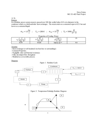
Figure 1: Rankine Cycle
Figure 2: Temperature/Enthalpy Rankine Diagram
2. Find:
(a) What is the water outlet Temperature?
In an ideal Rankine cycle, the heat dissipated in the condenser can be modelled as:
(1) 𝑞 = 𝑚̇ (ℎ2 − ℎ3)
Where 𝑚̇ is the mass flow rate of the hot working fluid; and ℎ2 and ℎ3 are the enthalpy values associated
with the hot working fluid at the given pressure at points 2 and 3, in this case 0.51 bar and conveniently
corresponding to the saturated liquid and saturated vapor states. These states are indicated by the
numbered locations in figures 1 and 2 and can be obtained from steam tables.
Plugging in values to equation 1:
𝑞ℎ𝑜𝑡 = 1.5
𝑘𝑔
𝑠
(2645.9 − 340.49)
𝑘𝐽
𝑘𝑔
= 3458.115 𝑘𝑊
𝑞ℎ𝑜𝑡 = 𝑞 𝑐𝑜𝑙𝑑 so to find the water outlet temperature we can use
(2) 𝑞 𝑐𝑜𝑙𝑑 = 𝑚̇ 𝑤 𝑐 𝑝,𝑤(𝑇𝑜 − 𝑇𝑖)
We know all values but 𝑇𝑜 so just need to rearrange, plug in values and solve:
𝑇𝑜 =
𝑞
𝑚̇ 𝑤 𝑐 𝑝,𝑤
+ 𝑇𝑖 =
3458115 𝑊
15
𝑘𝑔
𝑠
(4178
𝐽
𝑘𝑔∙𝐾
)
+ 280 𝐾
(b) What is the required tube length?
The general procedure will be to find the universal heat transfer coefficient (U) defined as:
(3) 𝑈 =
1
1
ℎ 𝑜
+
1
ℎ 𝑖
Where ℎ 𝑜 and ℎ 𝑖 are the convection coefficients on the outside and inside of the thin walled tubes.
The outside transfer coefficient is known. In order to find the inside coefficient we must find the Nusselt
number, Nu, defined as:
(4) 𝑁𝑢 =
ℎ𝐷
𝑘 𝑓
The Nusselt number is a function of the Reynolds and Pruitt number. The Pruitt number of the cooling
water is known so the Reynolds number needs to be found. For a circular pipe with fully developed flow
the Reynolds number is
(4) 𝑅𝑒 𝐷 =
4𝑚̇
𝜋𝐷𝜇
𝑇𝑜 = 335.12 𝐾 = 62° C
3. All the values are known so
𝑅𝑒 𝐷 =
4𝑚̇
𝜋𝐷𝜇
=
4 (
15 𝑘𝑔
100 𝑡𝑢𝑏𝑒𝑠 𝑠
)
𝜋(0.01𝑚)(700 X 10−6 𝑘𝑔
𝑚 ∙ 𝑠
)
= 27,283.7
For internal flow a Reynolds number 𝑅𝑒 ≥ 2300 is associated with turbulent flow. Looking at Table 8-41
it can be seen that the appropriate equation for the Nusselt number is
(5) 𝑁𝑢 𝐷 = 0.023𝑅𝑒4/5 𝑃𝑟 𝑛
Where n = 0.4 for cold to hot convection. So the Nusselt number is
𝑁𝑢 𝐷 = 0.023𝑅𝑒
4
5 𝑃𝑟 𝑛 = 0.023 (27283.7
4
5)4.60.4 = 150
The inside convection coefficient can be calculated from Equation 4 as
ℎ 𝑖 =
𝑁𝑢 ∙ 𝑘 𝑓
𝐷
=
150 (0.628
𝑊
𝑚 ∙ 𝐾
)
0.01 𝑚
= 9,420
𝑊
𝑚2 ∙ 𝐾
Now that the convection coefficients are known the universal heat transfer coefficient can be calculated
from Equation 3:
𝑈 =
1
1
ℎ 𝑜
+
1
ℎ 𝑖
=
1
1
5000
+
1
9420
= 3,266
𝑊
𝑚2 ∙ 𝐾
To find the length of each tube we must use the effectiveness method from the equation
(6) 𝑁𝑇𝑈( 𝑛𝑢𝑚𝑏𝑒𝑟 𝑜𝑓 𝑡𝑟𝑎𝑛𝑠𝑓𝑒𝑟 𝑢𝑛𝑖𝑡𝑠) =
𝑈𝐴
𝐶 𝑚𝑖𝑛
In order to do so we first need to find the heat capacitance C of each fluid which will give us 𝐶 𝑚𝑖𝑛 and a
heat capacitance ratio that will allow to find NTU.
(7) 𝐶 = 𝑚̇ 𝑐 𝑝
Because the hot fluid undergoes a phase change the temperature does not change. Specific heat is defined
as
𝑐ℎ𝑎𝑛𝑔𝑒 𝑖𝑛 𝑒𝑛𝑒𝑟𝑔𝑦
𝑐ℎ𝑎𝑛𝑔𝑒 𝑖𝑛 𝑡𝑒𝑚𝑝𝑒𝑟𝑎𝑡𝑢𝑟𝑒
so 𝑐 𝑝,ℎ = ∞
𝐶ℎ = 𝑚ℎ̇ 𝑐 𝑝,ℎ = 1.5
𝑘𝑔
𝑠
∞ = ∞
𝐶 𝑐 = 𝑚 𝑐̇ 𝑐 𝑝,𝑐 = 15
𝑘𝑔
𝑠
(4178
𝐽
𝑘𝑔 ∙ 𝐾
) = 62,670
𝑊
𝐾
4. These results show that 𝐶 𝑐 = 𝐶 𝑚𝑖𝑛 because it is smaller. The heat capacity ratio will give us our NTU:
(8) 𝐶𝑟 =
𝐶 𝑚𝑖𝑛
𝐶 𝑚𝑎𝑥
=
62,670
∞
= 0
We can now consult table 8-41
and observe that when 𝐶 𝑟 = 0, NTU is given by:
(9) 𝑁𝑇𝑈 = −𝑙𝑛(1 − 𝜀)
The efficiency, ε, is needed still and is given by:
(10) 𝜀 =
𝑞
𝑞 𝑚𝑎𝑥
Where q is the previously found heat transfer rate and 𝑞 𝑚𝑎𝑥 is:
(11) 𝑞 𝑚𝑎𝑥 = 𝐶 𝑚𝑖𝑛( 𝑇ℎ,𝑖 − 𝑇𝑐,1) = 62,670
𝑊
𝐾
(354.48 𝐾 − 280 𝐾) = 4,667.66 𝑘𝑊
So substituting in our efficiency into equation 9, our NTU becomes
𝑁𝑇𝑈 = −𝑙𝑛 (1 −
3458.115 𝑘𝑊
4.667.66 𝑘𝑊
) = 1.35
We can finally solve for our tube length by substituting values into equation 6 and solving for L:
𝑁𝑇𝑈 =
𝑈𝐴
𝐶 𝑚𝑖 𝑛
=
𝑈𝜋𝐷𝐿
𝐶 𝑚𝑖𝑛
𝐿 =
𝑁𝑇𝑈 ∙ 𝐶 𝑚𝑖𝑛
𝑈𝜋𝐷
=
(1.35) (62,670
𝑊
𝐾
)
3,266
𝑊
𝑚2 ∙ 𝐾
∙ 𝜋(0.01𝑚)
= 824.57 𝑚
(c)
With an accumulated fouling factor of 𝑅 𝑓 = 0.0003
𝑚2∙K
𝑊
, and using calculated length and inlet conditions,
what mass fraction of vapor is condensed?
Because the previous un-fouled system condensed all of the steam into water we can consider the former
condensed amount 100%. All we need to do is find the fouled efficiency and compare the ratios. The
overall heat transfer coefficient with fouling is
𝑈𝑓 = (
1
1
𝑈
+ 𝑅 𝑓
) = (
1
1
3266
+ 0.0003
) = 1650
𝑊
𝑚2 ∙ 𝐾
824.57
100
𝑚
𝑡𝑢𝑏𝑒
= 8.25
𝑚
𝑡𝑢𝑏𝑒
5. Our new NTU can be found using equation 6:
𝑁𝑇𝑈 =
𝑈𝐴
𝐶 𝑚𝑖𝑛
=
1650 ∙ 𝜋 ∙ (0.01)(824.57)
62,670
= 0.682
We can find our effectiveness by rearranging equation 9:
𝜀 𝑓 =
−1
𝑒 𝑁𝑇𝑈 + 1 =
−1
𝑒0.680 + 1 = 0.4944
The former efficiency was
𝜀 𝑢−𝑓 =
3458.115
4.667.66
= 0.7409
So our mass fraction condensed is
(d)
With tube length from (b) and fouling from (c), explore the extent to which the water flow rate and inlet
temperature can be varied to improve the condenser performance. Show results graphically.
*Note: I am very confused with this problem, if my 𝑚̇ changes, it effects many other variables.
My argument will be that as 𝑚̇ 𝑐 changes, so does Reynolds, Nusselt, convection coefficient, overall heat
transfer coefficient, NTU, and finally effectiveness.
Data in Appendix
0
0.1
0.2
0.3
0.4
0.5
0.6
0.7
0.8
0.9
1
0 5 10 15 20 25 30 35
Effectiveness
Mass Flow Rate of Cooling Water, kg/s
Mass Flow Rate of Cooling Water vs. Effectiveness
𝜀 𝑢−𝑓
𝜀 𝑓
=
0.7409
0.4944
= 0.667
6. 13.55
Known:
Two concentric spheres are separated by an air space.
𝐷1 = 0.8 𝑚; 𝐷2 = 1.2 𝑚; 𝑇1 = 400 𝐾; 𝑇2 = 300 𝐾
Diagram:
Assume:
- Steady State
Find:
(a) If the surfaces are black,what is the net rate of radiation exchange between the surfaces?
This can be calculated with:
(11) 𝑞 = 𝐴𝜎(𝑇𝑠
4 − 𝑇𝑠𝑢𝑟
4 )
Where 𝜎 ≡ 𝑡ℎ𝑒 𝑆𝑡𝑒𝑓𝑎𝑛 − 𝐵𝑜𝑙𝑡𝑧𝑚𝑎𝑛𝑛 𝐶𝑜𝑛𝑠𝑡𝑎𝑛𝑡 = 5.670 𝑋
10−8 𝑊
𝑚2∙𝐾4
. Solving equation 11:
𝑞 = 𝜋0.8𝑚2 (5.670 𝑋10−8
𝑊
𝑚2 ∙ 𝐾4 .) (400 𝐾4 − 300 𝐾4)
(b)
What is the net rate of radiation exchange if they are diffuse and gray and 𝜀1 = 0.5 and 𝜀2 = 0.05?
From Table 13.31
the heat flux for concentric spheres is
(12) 𝑞12 =
𝜎𝐴( 𝑇1
4
− 𝑇2
4)
1
𝜀1
+
1 − 𝜀2
𝜀2
(
𝑟1
𝑟2
)
2
So
𝑞 = 1995 𝑊
7. 𝑞12 =
(5.670 ∙ 10−8) 𝜋0.82(100 𝐾)
1
0.5
+
1 − 0.05
0.05
(
0.8
1.2
)
2 = 191 𝑊
(c)
What is the net rate of radiation exchange if 𝐷2 is increased to 20 m, with 𝜀1 = 0.5 and 𝜀2 = 0.05, and
𝐷2 = 0.8 𝑚?
Can just plug in additional value to equation 12 :
𝑞12 =
(5.670 ∙ 10−8) 𝜋0.82(100 𝐾)
1
0.5
+
1 − 0.05
0.05
(
0.8
20
)
2 = 982.6 𝑊
What error introduced if 𝜀2 = 1?
Using equation 12 again we get:
𝑞12 =
(5.670 ∙ 10−8) 𝜋0.82(1.75 ∙ 1010 )
1
0.5
+
1 − 1
1
(
0.8
20
)
2 = 997.5 𝑊
(d)
For 𝐷2 = 1.2 𝑚 and emissivities of 𝜀1 = 0.1,0.5, 𝑎𝑛𝑑 1.0, compute and plot the net rate of radiation
exchange as a function of 𝜀2 𝑓𝑜𝑟 0.05 ≤ 𝜀2 ≤ 1.0.
𝑞12 = 191 𝑊
𝑞12 = 982.6 𝑊
100 −
982.6
997.5
∙ 100 = 1.5%
8. Data in Appendix
0
50
100
150
200
250
0 0.2 0.4 0.6 0.8 1
q, W
ε2
Rate of Radiation, ε1 = 0.1
0
200
400
600
800
1000
1200
0 0.2 0.4 0.6 0.8 1
q, W
ε2
Radiation Rate, ε1 = 0.5
0
500
1000
1500
2000
2500
0 0.2 0.4 0.6 0.8 1
q, W
ε2
Radiation Rate, ε1 = 1.0
9. 13.112
Known:
There is a double paned window separated by atmospheric air for which the critical Raleigh number for
the onset of convection is 𝑅𝑎 = 2000.
𝑇1 = 22℃ ; 𝑇2 = −20℃
Diagram:
Assume:
- Isothermal Surfaces
- Steady State
- Quiescent Air
- Air is dry and at 1 atm
Find:
(a)
What is the conduction heat flux across the air gap for the optimal spacing 𝐿 𝑜𝑝 between the panes?
For this first part we are just dealing with conduction heat flux through the air so need to first find the
properties of the air at the mean temperature:
𝑇 𝑚 =
𝑇1 + 𝑇2
2
=
22 + (−20)
2
= 1℃
From Table A-41
𝜈 ∙ 106 (
𝑚2
𝑠
) 𝛼 ∙ 106 (
𝑚2
𝑠
) 𝛽 ( 𝐾−1)(
1
𝑇 𝑚
) 𝑘 ∙ 103 (
𝑊
𝑚 ∙ 𝐾
)
13.67 19.2 0.003648 24.3
The critical Rayleigh Number, where free convection will turn turbulent, is given as 2000. Using the
definition of the Rayleigh number I think I just need to solve for x:
(13) 𝑅𝑎 =
𝑔𝛽(𝑇2 − 𝑇1)𝑥3
𝛼 ∙ 𝜈
𝑥 = √
2000(19.2 ∙ 10−6)(13.64 ∙ 10−6)
9.8
𝑚
𝑠2 (0.003648 𝐾−1)(295.15 − 253.15)
3
= 0.00704 𝑚
10. So the conduction heat flux across it can be calculated with Fourier’s Law
(14) 𝑞̇ = 𝑘
∆𝑇
∆𝑥
Plugging in:
(b)
If the glass has an emissivity of 𝜀 𝑔 = 0.90, what is the total heat flux across the gap?
We can look at Table 13.31
again to get the equation we need parallel planes:
(15) 𝑞12 =
𝜎𝐴( 𝑇1
4
− 𝑇2
4)
1
𝜀1
+
1
𝜀2
− 1
With 𝜀1 = 𝜀2 = 0.9 and solving for heat flux instead of heat rate:
𝑞̇12 =
5.670 ∙ 10−8 𝑊
𝑚2 ∙ 𝐾4 (295.15 𝐾4 − 253.15 𝐾4)
1
0.9
+
1
0.9
− 1
= 161.3
𝑊
𝑚2
So total heat flux is the conduction from part (a) plus the radiation:
(c)
What is the total heat flux if a special, low emissivity coating (𝜀1 = 0.1) is applied to one of the panes at
its air glass interface? What is total heat flux if both panes are coated?
One Pane
Assuming the other pane still has an emissivity of 0.9 we can just plug into equation 15 with our new
value:
𝑞̇12 =
5.670 ∙ 10−8 𝑊
𝑚2 ∙ 𝐾4 (295.15 𝐾4 − 253.15 𝐾4)
1
0.9
+
1
0.1
− 1
= 19.5
𝑊
𝑚2
𝑞̇ = (0.0243
𝑊
𝑚 ∙ 𝐾
)
42℃
0.00704 𝑚
= 145
𝑊
𝑚2
𝑞̇ 𝑛𝑒𝑡 = 161.3 + 145 = 306.3
𝑊
𝑚2
11. Then add to the conduction:
Two Panes
Same procedure as with one pane but both emissivities equal to 0.1
𝑞̇12 =
5.670 ∙ 10−8 𝑊
𝑚2 ∙ 𝐾4 (295.15 𝐾4 − 253.15 𝐾4)
1
0.1
+
1
0.1
− 1
= 10.4
𝑊
𝑚2
And add to conduction
𝑞̇ 𝑛𝑒𝑡 = 19.5 + 145 = 164.5
𝑊
𝑚2
𝑞̇ 𝑛𝑒𝑡 = 10.4 + 145 = 155.4
𝑊
𝑚2