Download as PDF, PPTX

![Matlab Coding for pde
✓ m corresponds to m.
✓ xmesh(1) and xmesh(end) correspond to a and b.
✓ tspan(1) and tspan(end) correspond to t0 and tf.
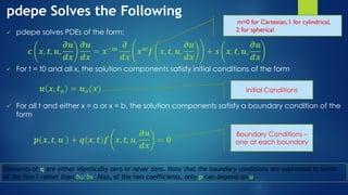
✓ pdefun computes the terms c, f, and s . It has the form
❖ [c,f,s] = pdefun(x,t,u,dudx)
✓ icfun evaluates the initial conditions. It has the form
❖ u = icfun(x)
✓ bcfun evaluates the terms p and q of the boundary conditions. It has the form
❖ [pl,ql,pr,qr] = bcfun(xl,ul,xr,ur,t)](https://image.slidesharecdn.com/solvingheatconductionequationparabolicpde-210513173631/85/Solving-heat-conduction-equation-parabolic-pde-7-320.jpg)


![Code Cont…
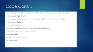
%now we will code all the program required to get the solution of pde
%our pde function
function [c,f,s]=pdex1pde(x,t,u,DuDx)
global alpha
c=1/alpha;
f=DuDx;
s=0;
%intial condion
function u0=pdex1ic(x,t,u,DuDx)
u0=20;
%boundary function
function [pl,ql,pr,qr]=pdex1bc(xl,ul,xr,ur,t)
pl=ul-100;
ql=0;
pr=ur-25;
qr=0;
% now we are ready to get the solution
%we can also get numerical soultion instead of plot](https://image.slidesharecdn.com/solvingheatconductionequationparabolicpde-210513173631/85/Solving-heat-conduction-equation-parabolic-pde-13-320.jpg)


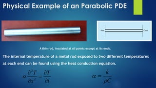
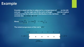
This document discusses solving a parabolic partial differential equation (PDE) describing heat conduction using the MATLAB PDE solver. It provides an example of using the pdepe solver to find the temperature distribution in a steel rod over time, given the boundary temperatures and properties of the rod. The document includes the equations, initial and boundary conditions, and MATLAB code used to set up and solve the PDE numerically using pdepe.


![Esercizio semicirconferenze tangenti [sc]](https://cdn.slidesharecdn.com/ss_thumbnails/esercizio-semicirconferenzetangentisc-210926212109-thumbnail.jpg?width=640&height=640&fit=bounds)


![[Deck] What's New in Spark-Iceberg Integration via DSV2.pptx](https://cdn.slidesharecdn.com/ss_thumbnails/deckwhatsnewinspark-icebergintegrationviadsv2-260210005337-25955b12-thumbnail.jpg?width=640&height=640&fit=bounds)


