Downloaded 8,988 times
![Chapter 1 • Introduction 3
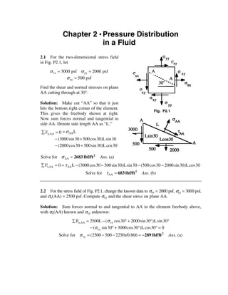
where the latter form follows from the ideal-gas law, ρ = p/RT. What are the dimensions
of the constant “1.26”? Estimate the mean free path of air at 20°C and 7 kPa. Is air
rarefied at this condition?
Solution: We know the dimensions of every term except “1.26”:
ìMü ìMü ì L2 ü
{l} = {L} {µ} = í ý {ρ} = í 3 ý {R} = í 2 ý {T} = {Θ}
î LT þ îL þ îT Θþ
Therefore the above formula (first form) may be written dimensionally as
{M/L⋅T}
{L} = {1.26?} = {1.26?}{L}
{M/L } √ [{L2 /T 2 ⋅ Θ}{Θ}]
3
Since we have {L} on both sides, {1.26} = {unity}, that is, the constant is dimensionless.
The formula is therefore dimensionally homogeneous and should hold for any unit system.
For air at 20°C = 293 K and 7000 Pa, the density is ρ = p/RT = (7000)/[(287)(293)] =
0.0832 kg/m3. From Table A-2, its viscosity is 1.80E−5 N ⋅ s/m2. Then the formula predict
a mean free path of
1.80E−5
l = 1.26 ≈ 9.4E−7 m Ans.
(0.0832)[(287)(293)]1/2
This is quite small. We would judge this gas to approximate a continuum if the physical
scales in the flow are greater than about 100 l, that is, greater than about 94 µm.
1.6 If p is pressure and y is a coordinate, state, in the {MLT} system, the dimensions of
the quantities (a) ∂p/∂y; (b) ò p dy; (c) ∂ 2 p/∂y2; (d) ∇p.
Solution: (a) {ML−2T−2}; (b) {MT−2}; (c) {ML−3T−2}; (d) {ML−2T−2}
1.7 A small village draws 1.5 acre-foot of water per day from its reservoir. Convert this
water usage into (a) gallons per minute; and (b) liters per second.
Solution: One acre = (1 mi2/640) = (5280 ft)2/640 = 43560 ft2. Therefore 1.5 acre-ft =
65340 ft3 = 1850 m3. Meanwhile, 1 gallon = 231 in3 = 231/1728 ft3. Then 1.5 acre-ft of
water per day is equivalent to
ft 3 æ 1728 gal ö æ 1 day ö gal
Q = 65340 ç 3 ÷ç ÷ ≈ 340 Ans. (a)
day è 231 ft ø è 1440 min ø min](https://image.slidesharecdn.com/solucionariodefluidoswhite-120604143132-phpapp02/85/Solucionario-de-fluidos_white-3-320.jpg)

![Chapter 1 • Introduction 5
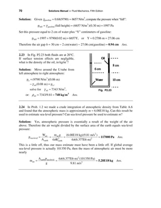
1.9 The dimensionless Galileo number, Ga, expresses the ratio of gravitational effect to
viscous effects in a flow. It combines the quantities density ρ, acceleration of gravity g,
length scale L, and viscosity µ. Without peeking into another textbook, find the form of
the Galileo number if it contains g in the numerator.
Solution: The dimensions of these variables are {ρ} = {M/L3}, {g} = {L/T2}, {L} =
{L}, and {µ} = {M/LT}. Divide ρ by µ to eliminate mass {M} and then combine with g
and L to eliminate length {L} and time {T}, making sure that g appears only to the first
power:
ì ρ ü ì M / L3 ü ì T ü
í ý=í ý=í 2ý
î µ þ î M / LT þ î L þ
while only {g} contains {T}. To keep {g} to the 1st power, we need to multiply it by
{ρ/µ}2. Thus {ρ/µ}2{g} = {T2/L4}{L/T2} = {L−3}.
We then make the combination dimensionless by multiplying the group by L3. Thus
we obtain:
2
æρö ρ 2 gL3 gL3
Galileo number = Ga = ç ÷ ( g)( L )3 = = 2 Ans.
èµø µ2 ν
1.10 The Stokes-Oseen formula [10] for drag on a sphere at low velocity V is:
9π
F = 3πµ DV + ρ V 2 D2
16
where D = sphere diameter, µ = viscosity, and ρ = density. Is the formula homogeneous?
Solution: Write this formula in dimensional form, using Table 1-2:
ì 9π ü
{F} = {3π }{µ}{D}{V} + í ý{ρ}{V}2 {D}2 ?
î 16 þ
ìMüì L ü
2
ì ML ü ìMü ìL ü
or: í 2 ý = {1} í ý{L} í ý + {1} í 3 ý í 2 ý {L2} ?
îT þ î LT þ îT þ îL þîT þ
where, hoping for homogeneity, we have assumed that all constants (3,π,9,16) are pure,
i.e., {unity}. Well, yes indeed, all terms have dimensions {ML/T2}! Therefore the Stokes-
Oseen formula (derived in fact from a theory) is dimensionally homogeneous.](https://image.slidesharecdn.com/solucionariodefluidoswhite-120604143132-phpapp02/85/Solucionario-de-fluidos_white-5-320.jpg)
![6 Solutions Manual • Fluid Mechanics, Fifth Edition
1.11 Test, for dimensional homogeneity, the following formula for volume flow Q
through a hole of diameter D in the side of a tank whose liquid surface is a distance h
above the hole position:
Q = 0.68D2 gh
where g is the acceleration of gravity. What are the dimensions of the constant 0.68?
Solution: Write the equation in dimensional form:
ì L3 ü ? 2 ì L ü
1/ 2
ì L3 ü
{Q} = í ý = {0.68?}{L } í 2 ý {L} 1/ 2
= {0.68} í ý
îTþ îT þ îTþ
Thus, since D2 ( gh ) has provided the correct volume-flow dimensions, {L3/T}, it follows
that the constant “0.68” is indeed dimensionless Ans. The formula is dimensionally
homogeneous and can be used with any system of units. [The formula is very similar to the
valve-flow formula Q = Cd A o (∆p/ ρ ) discussed at the end of Sect. 1.4, and the number
“0.68” is proportional to the “discharge coefficient” Cd for the hole.]
1.12 For low-speed (laminar) flow in a tube of radius ro, the velocity u takes the form
∆p 2 2
u=B
µ
(
ro − r )
where µ is viscosity and ∆p the pressure drop. What are the dimensions of B?
Solution: Using Table 1-2, write this equation in dimensional form:
{∆p} 2 ìL ü {M/LT 2} 2 ì L2 ü
{u} = {B} {r }, or: í ý = {B?} {L } = {B?} í ý ,
{µ} îT þ {M/LT} îTþ
or: {B} = {L–1} Ans.
The parameter B must have dimensions of inverse length. In fact, B is not a constant, it
hides one of the variables in pipe flow. The proper form of the pipe flow relation is
∆p 2 2
u=C
Lµ
(
ro − r )
where L is the length of the pipe and C is a dimensionless constant which has the
theoretical laminar-flow value of (1/4)—see Sect. 6.4.](https://image.slidesharecdn.com/solucionariodefluidoswhite-120604143132-phpapp02/85/Solucionario-de-fluidos_white-6-320.jpg)
![10 Solutions Manual • Fluid Mechanics, Fifth Edition
Solution: List the dimensions: {α} = {L2/T}, {L} = {L}, {µ} = {M/LT}, {δY} = {M/T2}.
We divide δ Y by µ to get rid of mass dimensions, then divide by α to eliminate time:
ìδ Y ü
í ý= 2
î µ þ T M
{
M LT
} ìL ü
= í ý , then í
îT þ
ìδ Y 1 ü ì L T ü ì 1 ü
ý=í =
2ý í ý
î µ α þ îT L þ î L þ
δ YL
Multiply by L and we obtain the Marangoni number: M = Ans.
µα
1.20C (“C” means computer-oriented, although this one can be done analytically.) A
baseball, with m = 145 g, is thrown directly upward from the initial position z = 0 and
Vo = 45 m/s. The air drag on the ball is CV2, where C ≈ 0.0010 N ⋅ s2/m2. Set up a
differential equation for the ball motion and solve for the instantaneous velocity V(t) and
position z(t). Find the maximum height zmax reached by the ball and compare your results
with the elementary-physics case of zero air drag.
Solution: For this problem, we include the weight of the ball, for upward motion z:
V t
dV dV
å Fz = −ma z , or: −CV − mg = m ò = − ò dt = −t
2
, solve
dt Vo
g + CV 2 /m 0
mg æ Cg ö m é cos(φ − t √ (gC/m) ù
Thus V = tan ç φ − t
ç ÷ and z = ln ê ú
C è m ÷ø C ë cosφ û
where φ = tan –1[Vo √ (C/mg)] . This is cumbersome, so one might also expect some
students simply to program the differential equation, m(dV/dt) + CV2 = −mg, with a
numerical method such as Runge-Kutta.
For the given data m = 0.145 kg, Vo = 45 m/s, and C = 0.0010 N⋅s2/m2, we compute
mg m Cg m
φ = 0.8732 radians, = 37.72 , = 0.2601 s−1 , = 145 m
C s m C
Hence the final analytical formulas are:
æ mö
V ç in ÷ = 37.72 tan(0.8732 − .2601t)
è sø
é cos(0.8732 − 0.2601t) ù
and z(in meters) = 145 ln ê ú
ë cos(0.8732) û
The velocity equals zero when t = 0.8732/0.2601 ≈ 3.36 s, whence we evaluate the
maximum height of the baseball as zmax = 145 ln[sec(0.8734)] ≈ 64.2 meters. Ans.](https://image.slidesharecdn.com/solucionariodefluidoswhite-120604143132-phpapp02/85/Solucionario-de-fluidos_white-10-320.jpg)
![Chapter 1 • Introduction 11
For zero drag, from elementary physics formulas, V = Vo − gt and z = Vot − gt2/2, we
calculate that
Vo 45 V2 (45)2
t max height = = ≈ 4.59 s and z max = o = ≈ 103.2 m
g 9.81 2g 2(9.81)
Thus drag on the baseball reduces the maximum height by 38%. [For this problem I
assumed a baseball of diameter 7.62 cm, with a drag coefficient CD ≈ 0.36.]
1.21 The dimensionless Grashof number, Gr, is a combination of density ρ, viscosity µ,
temperature difference ∆T, length scale L, the acceleration of gravity g, and the
coefficient of volume expansion β, defined as β = (−1/ρ)(∂ρ/∂T)p. If Gr contains both g
and β in the numerator, what is its proper form?
Solution: Recall that {µ/ρ} = {L2/T} and eliminates mass dimensions. To eliminate tem-
perature, we need the product {β∆Τ} = {1}. Then {g} eliminates {T}, and L3 cleans it all up:
Thus the dimensionless Gr = ρ 2 gβ∆TL3 /µ 2 Ans.
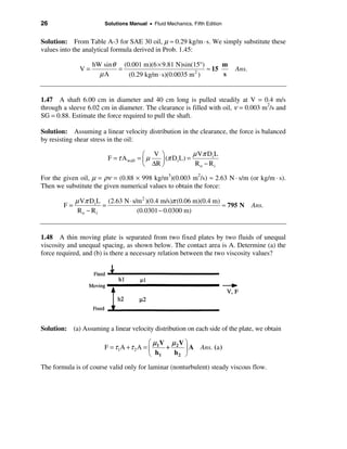
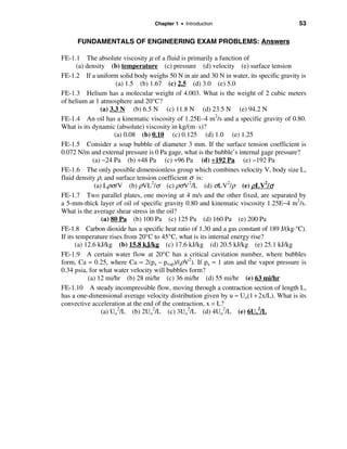
1.22* According to the theory of Chap. 8,
as a uniform stream approaches a cylinder
of radius R along the line AB shown in
Fig. P1.22, –∞ < x < –R, the velocities are
u = U ∞ (1 − R 2 /x 2 ); v = w = 0
Fig. P1.22
Using the concepts from Ex. 1.5, find (a) the maximum flow deceleration along AB; and
(b) its location.
Solution: We see that u slows down monotonically from U∞ at A to zero at point B,
x = −R, which is a flow “stagnation point.” From Example 1.5, the acceleration (du/dt) is
du ∂ u ∂u æ R2 ö é æ 2R 2 ö ù U 2 æ 2 2 ö x
= +u = 0 + U∞ ç1 − 2 ÷ ê U∞ ç + 3 ÷ú = ∞ ç 3 − 5 ÷ , ζ =
dt ∂ t ∂x è x øê ë è x øú R è ζ
û ζ ø R
This acceleration is negative, as expected, and reaches a minimum near point B, which is
found by differentiating the acceleration with respect to x:
d æ du ö 2 5
ç ÷ = 0 if ζ = , or
x
|max decel. ≈ −1.291 Ans. (b)
dx è dt ø 3 R
2
Substituting ζ = −1.291 into (du/dt) gives
du
|min = −0.372 U∞ Ans. (a)
dt R](https://image.slidesharecdn.com/solucionariodefluidoswhite-120604143132-phpapp02/85/Solucionario-de-fluidos_white-11-320.jpg)

![14 Solutions Manual • Fluid Mechanics, Fifth Edition
1.27 Given temperature and specific volume data for steam at 40 psia [Ref. 13]:
T, °F: 400 500 600 700 800
v, ft3/lbm: 12.624 14.165 15.685 17.195 18.699
Is the ideal gas law reasonable for this data? If so, find a least-squares value for the gas
constant R in m2/(s2⋅K) and compare with Table A-4.
Solution: The units are awkward but we can compute R from the data. At 400°F,
pV (40 lbf/in 2 )(144 in 2 /ft 2 )(12.624 ft 3 /lbm)(32.2 lbm/slug) ft⋅lbf
“R”400° F = = ≈ 2721
T (400 + 459.6)°R slug°R
The metric conversion factor, from the inside cover of the text, is “5.9798”: Rmetric =
2721/5.9798 = 455.1 m2/(s2⋅K). Not bad! This is only 1.3% less than the ideal-gas approxi-
mation for steam in Table A-4: 461 m2/(s2⋅K). Let’s try all the five data points:
T, °F: 400 500 600 700 800
R, m2/(s2⋅K): 455 457 459 460 460
The total variation in the data is only ±0.6%. Therefore steam is nearly an ideal gas in
this (high) temperature range and for this (low) pressure. We can take an average value:
1 5 J
p = 40 psia, 400°F ≤ T ≤ 800°F: R steam ≈ å R i ≈ 458 kg ⋅ K ± 0.6% Ans.
5 i=1
With such a small uncertainty, we don’t really need to perform a least-squares analysis,
but if we wanted to, it would go like this: We wish to minimize, for all data, the sum of
the squares of the deviations from the perfect-gas law:
2
æ pV ö
5
∂E 5
æ pV ö
Minimize E = å ç R − i ÷ by differentiating = 0 = å2çR − i ÷
i =1 è Ti ø ∂R i =1 è Ti ø
p 5 Vi 40(144) é 12.624 18.699 ù
Thus R least-squares = å T = 5 ê 860°R + L + 1260°R ú (32.2)
5 i =1 i ë û
For this example, then, least-squares amounts to summing the (V/T) values and converting
the units. The English result shown above gives Rleast-squares ≈ 2739 ft⋅lbf/slug⋅°R. Convert
this to metric units for our (highly accurate) least-squares estimate:
R steam ≈ 2739/5.9798 ≈ 458 ± 0.6% J/kg⋅K Ans.](https://image.slidesharecdn.com/solucionariodefluidoswhite-120604143132-phpapp02/85/Solucionario-de-fluidos_white-14-320.jpg)

![16 Solutions Manual • Fluid Mechanics, Fifth Edition
1.30 Repeat Prob. 1.29 if the tank is filled with compressed water rather than air. Why
is the result thousands of times less than the result of 215,000 ft⋅lbf in Prob. 1.29?
Solution: First evaluate the density change of water. At 1 atm, ρ o ≈ 1.94 slug/ft3. At
120 psi(gage) = 134.7 psia, the density would rise slightly according to Eq. (1.22):
æ ρ ö
7
p 134.7
= ≈ 3001ç ÷ − 3000, solve ρ ≈ 1.940753 slug/ft ,
3
po 14.7 è 1.94 ø
Hence m water = ρυ = (1.940753)(5 ft 3 ) ≈ 9.704 slug
The density change is extremely small. Now the work done, as in Prob. 1.29 above, is
m dρ ∆ρ
2 2 2
æmö
W1-2 = −ò p dυ = ò pdç ÷ = ò p ≈ pavg m 2 for a linear pressure rise
èρø 1 ρ ρavg
2
1 1
æ 14.7 + 134.7 lbf ö æ 0.000753 ft 3 ö
Hence W1-2 ≈ ç × 144 2 ÷ (9.704 slug) ç ÷ ≈ 21 ft⋅ lbf Ans.
è 2 ft ø è 1.94042 slug ø
[Exact integration of Eq. (1.22) would give the same numerical result.] Compressing
water (extremely small ∆ρ) takes ten thousand times less energy than compressing air,
which is why it is safe to test high-pressure systems with water but dangerous with air.
1.31 The density of water for 0°C < T < 100°C is given in Table A-1. Fit this data to a
least-squares parabola, ρ = a + bT + cT2, and test its accuracy vis-a-vis Table A-1.
Finally, compute ρ at T = 45°C and compare your result with the accepted value of ρ ≈
990.1 kg/m3.
Solution: The least-squares parabola which fits the data of Table A-1 is:
ρ (kg/m3) ≈ 1000.6 – 0.06986T – 0.0036014T2, T in °C Ans.
When compared with the data, the accuracy is less than ±1%. When evaluated at the
particular temperature of 45°C, we obtain
ρ45°C ≈ 1000.6 – 0.06986(45) – 0.003601(45)2 ≈ 990.2 kg/m3 Ans.
This is excellent accuracya good fit to good smooth data.
The data and the parabolic curve-fit are shown plotted on the next page. The curve-fit
does not display the known fact that ρ for fresh water is a maximum at T = +4°C.](https://image.slidesharecdn.com/solucionariodefluidoswhite-120604143132-phpapp02/85/Solucionario-de-fluidos_white-16-320.jpg)
![Chapter 1 • Introduction 17
1.32 A blimp is approximated by a prolate spheroid 90 m long and 30 m in diameter.
Estimate the weight of 20°C gas within the blimp for (a) helium at 1.1 atm; and (b) air at
1.0 atm. What might the difference between these two values represent (Chap. 2)?
Solution: Find a handbook. The volume of a prolate spheroid is, for our data,
2 2
υ = π LR 2 = π (90 m)(15 m)2 ≈ 42412 m 3
3 3
Estimate, from the ideal-gas law, the respective densities of helium and air:
pHe 1.1(101350) kg
(a) ρ helium = = ≈ 0.1832 3 ;
R He T 2077(293) m
pair 101350 kg
(b) ρ air = = ≈ 1.205 3 .
R air T 287(293) m
Then the respective gas weights are
æ kg öæ mö
WHe = ρ He gυ = ç 0.1832 3 ÷ç 9.81 2 ÷ (42412 m 3 ) ≈ 76000 N Ans. (a)
è m øè s ø
Wair = ρ air gυ = (1.205)(9.81)(42412) ≈ 501000 N Ans. (b)
The difference between these two, 425000 N, is the buoyancy, or lifting ability, of the
blimp. [See Section 2.8 for the principles of buoyancy.]](https://image.slidesharecdn.com/solucionariodefluidoswhite-120604143132-phpapp02/85/Solucionario-de-fluidos_white-17-320.jpg)
![Chapter 1 • Introduction 19
For EES or the Steam Tables, just program the properties for steam or look it up:
EES real steam: ρ1 = 5.23 kg/m 3 Ans. (a), ρ2 = 2.16 kg/m 3 Ans. (b)
The ideal-gas error is only about 3%, even though the expansion approached the saturation line.
1.35 In Table A-4, most common gases (air, nitrogen, oxygen, hydrogen, CO, NO)
have a specific heat ratio k = 1.40. Why do argon and helium have such high values?
Why does NH3 have such a low value? What is the lowest k for any gas that you know?
Solution: In elementary kinetic theory of gases [8], k is related to the number of
“degrees of freedom” of the gas: k ≈ 1 + 2/N, where N is the number of different modes
of translation, rotation, and vibration possible for the gas molecule.
Example: Monotomic gas, N = 3 (translation only), thus k ≈ 5/3
This explains why helium and argon, which are monatomic gases, have k ≈ 1.67.
Example: Diatomic gas, N = 5 (translation plus 2 rotations), thus k ≈ 7/5
This explains why air, nitrogen, oxygen, NO, CO and hydrogen have k ≈ 1.40.
But NH3 has four atoms and therefore more than 5 degrees of freedom, hence k will
be less than 1.40 (the theory is not too clear what “N” is for such complex molecules).
The lowest k known to this writer is for uranium hexafluoride, 238UF6, which is a very
complex, heavy molecule with many degrees of freedom. The estimated value of k for
this heavy gas is k ≈ 1.06.
1.36 The bulk modulus of a fluid is defined as B = ρ (∂ p/∂ρ)S. What are the dimensions
of B? Estimate B (in Pa) for (a) N2O, and (b) water, at 20°C and 1 atm.
Solution: The density units cancel in the definition of B and thus its dimensions are the
same as pressure or stress:
ì M ü
{B} = {p} = {F/L2} = í 2 ý Ans.
î LT þ
(a) For an ideal gas, p = Cρ k for an isentropic process, thus the bulk modulus is:
d
Ideal gas: B = ρ (Cρ k ) = ρ kCρ k −1 = kCρ k = kp
dρ
For N 2 O, from Table A-4, k ≈ 1.31, so BN2O = 1.31 atm = 1.33E5 Pa Ans. (a)](https://image.slidesharecdn.com/solucionariodefluidoswhite-120604143132-phpapp02/85/Solucionario-de-fluidos_white-19-320.jpg)
![20 Solutions Manual • Fluid Mechanics, Fifth Edition
For water at 20°C, we could just look it up in Table A-3, but we more usefully try to
estimate B from the state relation (1-22). Thus, for a liquid, approximately,
d
B≈ ρ [po {(B + 1)( ρ / ρo )n − B}] = n(B + 1)p o ( ρ / ρ o )n = n(B + 1)p o at 1 atm
dρ
For water, B ≈ 3000 and n ≈ 7, so our estimate is
Bwater ≈ 7(3001)po = 21007 atm ≈ 2.13E9 Pa Ans. (b)
This is 2.7% less than the value B = 2.19E9 Pa listed in Table A-3.
1.37 A near-ideal gas has M = 44 and cv = 610 J/(kg⋅K). At 100°C, what are (a) its
specific heat ratio, and (b) its speed of sound?
Solution: The gas constant is R = Λ/Μ = 8314/44 ≈ 189 J/(kg⋅K). Then
c v = R/(k − 1), or: k = 1 + R/c v = 1 + 189/610 ≈ 1.31 Ans. (a) [It is probably N 2 O]
With k and R known, the speed of sound at 100ºC = 373 K is estimated by
a = kRT = 1.31[189 m 2 /(s2 ⋅ K)](373 K) ≈ 304 m/s Ans. (b)
1.38 In Fig. P1.38, if the fluid is glycerin
at 20°C and the width between plates is
6 mm, what shear stress (in Pa) is required
to move the upper plate at V = 5.5 m/s?
What is the flow Reynolds number if “L” is
taken to be the distance between plates?
Fig. P1.38
Solution: (a) For glycerin at 20°C, from Table 1.4, µ ≈ 1.5 N · s/m2. The shear stress is
found from Eq. (1) of Ex. 1.8:
µV (1.5 Pa⋅s)(5.5 m/s)
τ= = ≈ 1380 Pa Ans. (a)
h (0.006 m)
The density of glycerin at 20°C is 1264 kg/m3. Then the Reynolds number is defined by
Eq. (1.24), with L = h, and is found to be decidedly laminar, Re < 1500:
ρVL (1264 kg/m 3 )(5.5 m/s)(0.006 m)
Re L = = ≈ 28 Ans. (b)
µ 1.5 kg/m ⋅ s](https://image.slidesharecdn.com/solucionariodefluidoswhite-120604143132-phpapp02/85/Solucionario-de-fluidos_white-20-320.jpg)
![Chapter 1 • Introduction 21
1.39 Knowing µ ≈ 1.80E−5 Pa · s for air at 20°C from Table 1-4, estimate its viscosity at
500°C by (a) the Power-law, (b) the Sutherland law, and (c) the Law of Corresponding
States, Fig. 1.5. Compare with the accepted value µ(500°C) ≈ 3.58E−5 Pa · s.
Solution: First change T from 500°C to 773 K. (a) For the Power-law for air, n ≈ 0.7,
and from Eq. (1.30a),
0.7
æ 773 ö kg
µ = µo (T/To ) ≈ (1.80E − 5) ç
n
≈ 3.55E − 5 Ans. (a)
è 293 ÷
ø m⋅ s
This is less than 1% low. (b) For the Sutherland law, for air, S ≈ 110 K, and from Eq. (1.30b),
é (T/To )1.5 (To + S) ù é (773/293)1.5 (293 + 110) ù
µ = µo ê ú ≈ (1.80E − 5) ê ú
ë (T + S) û ë (773 + 110) û
kg
= 3.52E − 5 Ans. (b)
m⋅ s
This is only 1.7% low. (c) Finally use Fig. 1.5. Critical values for air from Ref. 3 are:
Air: µc ≈ 1.93E − 5 Pa⋅s Tc ≈ 132 K (“mixture” estimates)
At 773 K, the temperature ratio is T/Tc = 773/132 ≈ 5.9. From Fig. 1.5, read µ/µc ≈ 1.8.
Then our critical-point-correlation estimate of air viscosity is only 3% low:
kg
µ ≈ 1.8µc = (1.8)(1.93E−5) ≈ 3.5E−5 Ans. (c)
m⋅ s
1.40 Curve-fit the viscosity data for water in Table A-1 in the form of Andrade’s equation,
æ Bö
µ ≈ A exp ç ÷ where T is in °K and A and B are curve-fit constants.
èTø
Solution: This is an alternative formula to the log-quadratic law of Eq. (1.31). We have
eleven data points for water from Table A-1 and can perform a least-squares fit to
Andrade’s equation:
11
∂E ∂E
Minimize E = å [ µ i − A exp(B/Ti )]2 , then set = 0 and =0
i =1 ∂A ∂B
The result of this minimization is: A ≈ 0.0016 kg/m⋅s, B ≈ 1903°K. Ans.](https://image.slidesharecdn.com/solucionariodefluidoswhite-120604143132-phpapp02/85/Solucionario-de-fluidos_white-21-320.jpg)
![22 Solutions Manual • Fluid Mechanics, Fifth Edition
The data and the Andrade’s curve-fit are plotted. The error is ±7%, so Andrade’s
equation is not as accurate as the log-quadratic correlation of Eq. (1.31).
1.41 Some experimental values of µ for argon gas at 1 atm are as follows:
T, °K: 300 400 500 600 700 800
µ, kg/m · s: 2.27E–5 2.85E–5 3.37E–5 3.83E–5 4.25E–5 4.64E–5
Fit these values to either (a) a Power-law, or (b) a Sutherland law, Eq. (1.30a,b).
Solution: (a) The Power-law is straightforward: put the values of µ and T into, say,
“Cricket Graph”, take logarithms, plot them, and make a linear curve-fit. The result is:
0.73
æ T °K ö
Power-law fit: µ ≈ 2.29E −5 ç ÷ Ans. (a)
è 300 K ø
Note that the constant “2.29E–5” is slightly higher than the actual viscosity “2.27E–5”
at T = 300 K. The accuracy is ±1% and would be poorer if we replaced 2.29E–5 by
2.27E–5.
(b) For the Sutherland law, unless we rewrite the law (1.30b) drastically, we don’t
have a simple way to perform a linear least-squares correlation. However, it is no trouble
to perform the least-squares summation, E = Σ[µi – µo(Ti/300)1.5(300 + S)/(Ti + S)]2 and
minimize by setting ∂ E/∂ S = 0. We can try µo = 2.27E–5 kg/m⋅s for starters, and it works
fine. The best-fit value of S ≈ 143°K with negligible error. Thus the result is:
µ (T/300)1.5 (300 + 143 K)
Sutherland law: ≈ Ans. (b)
2.27E−5 kg/m⋅s (T + 143 K)](https://image.slidesharecdn.com/solucionariodefluidoswhite-120604143132-phpapp02/85/Solucionario-de-fluidos_white-22-320.jpg)
![Chapter 1 • Introduction 23
We may tabulate the data and the two curve-fits as follows:
T, °K: 300 400 500 600 700 800
µ × E5, data: 2.27 2.85 3.37 3.83 4.25 4.64
µ × E5, Power-law: 2.29 2.83 3.33 3.80 4.24 4.68
µ × E5, Sutherland: 2.27 2.85 3.37 3.83 4.25 4.64
1.42 Some experimental values of µ of helium at 1 atm are as follows:
T, °K: 200 400 600 800 1000 1200
µ, kg/m ⋅ s: 1.50E–5 2.43E–5 3.20E–5 3.88E–5 4.50E–5 5.08E–5
Fit these values to either (a) a Power-law, or (b) a Sutherland law, Eq. (1.30a,b).
Solution: (a) The Power-law is straightforward: put the values of µ and T into, say,
“Cricket Graph,” take logarithms, plot them, and make a linear curve-fit. The result is:
0.68
æ T °K ö
Power-law curve-fit: µ He ≈ 1.505E − 5 ç ÷ Ans. (a)
è 200 K ø
The accuracy is less than ±1%. (b) For the Sutherland fit, we can emulate Prob. 1.41 and
perform the least-squares summation, E = Σ[µi – µo(Ti/200)1.5(200 + S)/(Ti + S)]2 and
minimize by setting ∂ E/∂ S = 0. We can try µo = 1.50E–5 kg/m·s and To = 200°K for
starters, and it works OK. The best-fit value of S ≈ 95.1°K. Thus the result is:
µ Helium (T/200)1.5 (200 + 95.1° K)
Sutherland law: ≈ ± 4% Ans. (b)
1.50E−5 kg/m ⋅ s (T + 95.1° K)
For the complete range 200–1200°K, the Power-law is a better fit. The Sutherland law
improves to ±1% if we drop the data point at 200°K.
1.43 Yaws et al. [ref. 34] suggest a 4-constant curve-fit formula for liquid viscosity:
log10 µ ≈ A + B/T + CT + DT 2, with T in absolute units.
(a) Can this formula be criticized on dimensional grounds? (b) If we use the formula
anyway, how do we evaluate A,B,C,D in the least-squares sense for a set of N data points?](https://image.slidesharecdn.com/solucionariodefluidoswhite-120604143132-phpapp02/85/Solucionario-de-fluidos_white-23-320.jpg)
![24 Solutions Manual • Fluid Mechanics, Fifth Edition
Solution: (a) Yes, if you’re a purist: A is dimensionless, but B,C,D are not. It would be
more comfortable to this writer to write the formula in terms of some reference
temperature To:
log10 µ ≈ A + B(To /T) + C(T/To ) + D(T/To )2 , (dimensionless A,B,C,D)
(b) For least squares, express the square error as a summation of data-vs-formula
differences:
N N
2
E = å é A + B/Ti + CTi + DT 2 − log10 µ i ù = å f 2
ë i û i for short.
i =1 i =1
Then evaluate ∂ E /∂ A = 0, ∂ E /∂ B = 0, ∂ E /∂ C = 0, and ∂ E /∂ D = 0, to give four
simultaneous linear algebraic equations for (A,B,C,D):
å fi = 0; å fi /Ti = 0; å fi Ti = 0; å fi T 2 = 0,
i
where fi = A + B/Ti + CTi + DTi2 − log10 µ i
Presumably this was how Yaws et al. [34] computed (A,B,C,D) for 355 organic liquids.
1.44 The viscosity of SAE 30 oil may vary considerably, according to industry-agreed
specifications [SAE Handbook, Ref. 26]. Comment on the following data and fit the data
to Andrade’s equation from Prob. 1.41.
T, °C: 0 20 40 60 80 100
µSAE30, kg/m · s: 2.00 0.40 0.11 0.042 0.017 0.0095
Solution: At lower temperatures, 0°C < T < 60°C, these values are up to fifty per cent
higher than the curve labelled “SAE 30 Oil” in Fig. A-1 of the Appendix. However, at 100°C,
the value 0.0095 is within the range specified by SAE for this oil: 9.3 < ν < 12.5 mm2/s,
if its density lies in the range 760 < ρ < 1020 kg/m3, which it surely must. Therefore a
surprisingly wide difference in viscosity-versus-temperature still makes an oil “SAE 30.”
To fit Andrade’s law, µ ≈ A exp(B/T), we must make a least-squares fit for the 6 data points
above (just as we did in Prob. 1.41):
2
é 6
æ B öù ∂E ∂E
Andrade fit: With E = å ê µ i − A exp ç ÷ ú , then set = 0 and =0
i =1 ë è Ti ø û ∂A ∂B
This formulation produces the following results:
kg æ 6245 K ö
Least-squares of µ versus T: µ ≈ 2.35E−10 exp ç
è T° K ÷
Ans. (#1)
m⋅ s ø](https://image.slidesharecdn.com/solucionariodefluidoswhite-120604143132-phpapp02/85/Solucionario-de-fluidos_white-24-320.jpg)


![28 Solutions Manual • Fluid Mechanics, Fifth Edition
(b) Evaluate the two equations for the data. We need the net weight of the sphere in the fluid:
Wnet = ( ρsphere − ρfluid )g(Vol )fluid = (2700 − 875 kg/m 3)(9.81 m/s2 )(π /6)(0.0025 m)3
= 0.000146 N
Wnet t (0.000146 N )(32 s) kg
Then µ = = = 0.40 Ans. (b)
3π DL 3π (0.0025 m)(0.5 m) m⋅s
2ρDL 2(875 kg/m3)(0.0025 m)(0.5 m)
Check t = 32 s compared to =
µ 0.40 kg/m ⋅ s
= 5.5 s OK, t is greater
1.51 Use the theory of Prob. 1.50 for a shaft 8 cm long, rotating at 1200 r/min, with
ri = 2.00 cm and ro = 2.05 cm. The measured torque is M = 0.293 N·m. What is the fluid
viscosity? If the experimental uncertainties are: L (±0.5 mm), M (±0.003 N-m), Ω (±1%),
and ri and ro (±0.02 mm), what is the uncertainty in the viscosity determination?
Solution: First change the rotation rate to Ω = (2π/60)(1200) = 125.7 rad/s. Then the
analytical expression derived in Prob. 1.50 directly above is
M(R o − R i ) (0.293 N ⋅ m)(0.0205 − 0.0200 m) kg
µ= = ≈ 0.29 Ans.
2πΩR i L
3
æ rad ö m⋅ s
2π ç 125.7 3
÷ (0.02 m) (0.08 m)
è s ø
It might be SAE 30W oil! For estimating overall uncertainty, since the formula involves
five things, the total uncertainty is a combination of errors, each expressed as a fraction:
0.003 0.04
SM = = 0.0102; S∆R = = 0.08; SΩ = 0.01
0.293 0.5
æ 0.02 ö 0.5
SR3 = 3SR = 3 ç ÷ = 0.003; SL = = 0.00625
è 20 ø 80
One might dispute the error in ∆R—here we took it to be the sum of the two (±0.02-mm)
errors. The overall uncertainty is then expressed as an rms computation [Refs. 30 and 31
of Chap. 1]:
(
Sµ = √ S2 + S2 R + S2 + S2 3 + S2
m ∆ Ω R L )
= [(0.0102)2 + (0.08)2 + (0.01)2 + (0.003)2 + (0.00625)2 ] ≈ 0.082 Ans.](https://image.slidesharecdn.com/solucionariodefluidoswhite-120604143132-phpapp02/85/Solucionario-de-fluidos_white-28-320.jpg)

![Chapter 1 • Introduction 31
For uncertainty, looking at the formula for µ, we have first powers in h, M, and Ω and a
fourth power in R. The overall uncertainty estimate [see Eq. (1.44) and Ref. 31] would be
1/ 2
Sµ ≈ éS2 + S2 + S2 + (4SR )2 ù
ë h M Ω û
≈ [(0.01) + (0.01) + (0.01)2 + {4(0.01)}2 ]1/ 2 ≈ 0.044 or: ±4.4% Ans.
2 2
The uncertainty is dominated by the 4% error due to radius measurement. We might
report the measured viscosity as µ ≈ 0.29 ± 4.4% kg/m·s or 0.29 ± 0.013 kg/m·s.
1.56* For the cone-plate viscometer in
Fig. P1.56, the angle is very small, and the
gap is filled with test liquid µ. Assuming a
linear velocity profile, derive a formula for
the viscosity µ in terms of the torque M
and cone parameters. Fig. P1.56
Solution: For any radius r ≤ R, the liquid gap is h = r tanθ. Then
æ Ωr ö æ dr ö
d(Torque) = dM = τ dA w r = ç µ ÷ ç 2π r cosθ ÷ r, or
è r tanθ ø è ø
2πΩµ 2 2πΩµ R 3M sinθ
R 3
M= ò r dr = 3sinθ , or: µ = 2πΩR 3 Ans.
sin θ 0
1.57 Apply the cone-plate viscometer of Prob. 1.56 above to the special case R = 6 cm,
θ = 3°, M = 0.157 N ⋅ m, and a rotation rate of 600 rev/min. What is the fluid viscosity? If
each parameter (M,R,Ω,θ) has an uncertainty of ±1%, what is the uncertainty of µ?
Solution: We derived a suitable linear-velocity-profile formula in Prob. 1.56. Convert
the rotation rate to rad/s: Ω = (600 rev/min)(2π rad/rev ÷ 60 s/min) = 62.83 rad/s. Then,
3M sinθ 3(0.157 N ⋅ m)sin(3°) N⋅ s æ kg ö
µ= = = 0.29 ç or ÷ Ans.
2πΩR 3 2π (62.83 rad/s)(0.06 m)3 m2 è m ⋅ s ø
For uncertainty, looking at the formula for µ, we have first powers in θ, M, and Ω and a
third power in R. The overall uncertainty estimate [see Eq. (1.44) and Ref. 31] would be
1/ 2
Sµ = éSθ + S2 + S2 + (3SR )2 ù
ë
2
M Ω û
≈ [(0.01) + (0.01) + (0.01)2 + {3(0.01)}2 ]1/ 2 = 0.035, or: ±3.5%
2 2
Ans.
The uncertainty is dominated by the 3% error due to radius measurement. We might
report the measured viscosity as µ ≈ 0.29 ± 3.5% kg/m·s or 0.29 ± 0.01 kg/m·s.](https://image.slidesharecdn.com/solucionariodefluidoswhite-120604143132-phpapp02/85/Solucionario-de-fluidos_white-31-320.jpg)
![32 Solutions Manual • Fluid Mechanics, Fifth Edition
1.58 The laminar-pipe-flow example of Prob. 1.14 leads to a capillary viscometer [27],
using the formula µ = π r o4∆p/(8LQ). Given ro = 2 mm and L = 25 cm. The data are
Q, m3/hr: 0.36 0.72 1.08 1.44 1.80
∆p, kPa: 159 318 477 1274 1851
Estimate the fluid viscosity. What is wrong with the last two data points?
Solution: Apply our formula, with consistent units, to the first data point:
π ro4 ∆p π (0.002 m)4 (159000 N/m 2 ) N ⋅s
∆p = 159 kPa: µ ≈ = 3
≈ 0.040 2
8LQ 8(0.25 m)(0.36/3600 m /s) m
Do the same thing for all five data points:
∆p, kPa: 159 318 477 1274 1851
µ, N·s/m : 2
0.040 0.040 0.040 0.080(?) 0.093(?) Ans.
The last two estimates, though measured properly, are incorrect. The Reynolds number of the
capillary has risen above 2000 and the flow is turbulent, which requires a different formula.
1.59 A solid cylinder of diameter D, length L, density ρs falls due to gravity inside a tube of
diameter Do. The clearance, (Do − D) = D, is filled with a film of viscous fluid (ρ,µ). Derive
a formula for terminal fall velocity and apply to SAE 30 oil at 20°C for a steel cylinder with
D = 2 cm, Do = 2.04 cm, and L = 15 cm. Neglect the effect of any air in the tube.
Solution: The geometry is similar to Prob. 1.47, only vertical instead of horizontal. At
terminal velocity, the cylinder weight should equal the viscous drag:
π 2 é V ù
a z = 0: ΣFz = − W + Drag = − ρsg D L + êµ ú π DL,
4 ë (Do − D)/2 û
ρs gD (Do − D)
or: V = Ans.
8µ
For the particular numerical case given, ρsteel ≈ 7850 kg/m3. For SAE 30 oil at 20°C,
µ ≈ 0.29 kg/m·s from Table 1.4. Then the formula predicts
ρsgD(Do − D) (7850 kg/m 3 )(9.81 m/s2 )(0.02 m)(0.0204 − 0.02 m)
Vterminal = =
8µ 8(0.29 kg/m ⋅ s)
≈ 0.265 m/s Ans.](https://image.slidesharecdn.com/solucionariodefluidoswhite-120604143132-phpapp02/85/Solucionario-de-fluidos_white-32-320.jpg)

![34 Solutions Manual • Fluid Mechanics, Fifth Edition
x direction is the air drag resisting the motion, assuming a linear velocity distribution in
the air:
V dV
å Fx = −τ A = − µ A=m , where h = air film thickness
h dt
Separate the variables and integrate to find the velocity of the decelerating puck:
µA
V t
dV
ò = −K ò dt, or V = Vo e − Kt , where K =
Vo
V 0
mh
Integrate again to find the displacement of the puck:
t
Vo
x = ò V dt = [1 − e − Kt ]
0
K
Apply to the particular case given: air, µ ≈ 1.8E−5 kg/m·s, m = 50 g, D = 9 cm, h = 0.12 mm,
Vo = 10 m/s. First evaluate the time-constant K:
µ A (1.8E−5 kg/m ⋅ s)[(π /4)(0.09 m)2 ]
K= = ≈ 0.0191 s −1
mh (0.050 kg)(0.00012 m)
(a) When the puck slows down to 1 m/s, we obtain the time:
−1
V = 1 m/s = Vo e − Kt = (10 m/s) e −(0.0191 s )t
, or t ≈ 121 s Ans. (a)
(b) The puck will stop completely only when e–Kt = 0, or: t = ∞ Ans. (b)
(c) For part (a), the puck will have travelled, in 121 seconds,
Vo 10 m/s
x= (1 − e − Kt ) = −1
[1 − e −(0.0191)(121) ] ≈ 472 m Ans. (c)
K 0.0191 s
This may perhaps be a little unrealistic. But the air-hockey puck does accelerate slowly!
1.62 The hydrogen bubbles in Fig. 1.13 have D ≈ 0.01 mm. Assume an “air-water”
interface at 30°C. What is the excess pressure within the bubble?
Solution: At 30°C the surface tension from Table A-1 is 0.0712 N/m. For a droplet or
bubble with one spherical surface, from Eq. (1.32),
2Y 2(0.0712 N/m)
∆p = = ≈ 28500 Pa Ans.
R (5E−6 m)](https://image.slidesharecdn.com/solucionariodefluidoswhite-120604143132-phpapp02/85/Solucionario-de-fluidos_white-34-320.jpg)
![Chapter 1 • Introduction 37
Solution: For the figure above, the force balance on the annular fluid is
( )
Y cosθ (2π ro + 2π ri ) = ρ gπ ro − ri2 h
2
Cancel where possible and the result is
h = 2Y cosθ /{ ρ g(ro − ri )} Ans.
1.68* Analyze the shape η(x) of the
water-air interface near a wall, as shown.
Assume small slope, R−1 ≈ d2η/dx2. The
pressure difference across the interface is
∆p ≈ ρgη, with a contact angle θ at x = 0
and a horizontal surface at x = ∞. Find an Fig. P1.68
expression for the maximum height h.
Solution: This is a two-dimensional surface-tension problem, with single curvature. The
surface tension rise is balanced by the weight of the film. Therefore the differential equation is
Y d 2η æ dη ö
∆p = ρ gη = ≈Y 2 ç = 1÷
R dx è dx ø
This is a second-order differential equation with the well-known solution,
η = C1 exp[Kx] + C2 exp[ −Kx], K = ( ρ g/Y)
To keep η from going infinite as x = ∞, it must be that C1 = 0. The constant C2 is found
from the maximum height at the wall:
η|x =0 = h = C2 exp(0), hence C2 = h
Meanwhile, the contact angle shown above must be such that,
dη
|x=0 = −cot(θ ) = −hK, thus h = cotθ
dx K](https://image.slidesharecdn.com/solucionariodefluidoswhite-120604143132-phpapp02/85/Solucionario-de-fluidos_white-37-320.jpg)
![38 Solutions Manual • Fluid Mechanics, Fifth Edition
The complete (small-slope) solution to this problem is:
η = h exp[− ( ρ g/Y)1/2 x], where h = (Y/ρg)1/2 cotθ Ans.
The formula clearly satisfies the requirement that η = 0 if x = ∞. It requires “small slope”
and therefore the contact angle should be in the range 70° < θ < 110°.
1.69 A solid cylindrical needle of diameter
d, length L, and density ρn may “float” on a
liquid surface. Neglect buoyancy and assume
a contact angle of 0°. Calculate the maxi-
mum diameter needle able to float on the
Fig. P1.69
surface.
Solution: The needle “dents” the surface downward and the surface tension forces are
upward, as shown. If these tensions are nearly vertical, a vertical force balance gives:
π 8Y
å Fz = 0 = 2YL − ρ g d 2 L, or: d max ≈ Ans. (a)
4 πρ g
(b) Calculate dmax for a steel needle (SG ≈ 7.84) in water at 20°C. The formula becomes:
8Y 8(0.073 N/m)
d max = = ≈ 0.00156 m ≈ 1.6 mm Ans. (b)
πρg π (7.84 × 998 kg/m 3 )(9.81 m/s2 )
1.70 Derive an expression for the capillary-
height change h, as shown, for a fluid of
surface tension Y and contact angle θ be-
tween two parallel plates W apart. Evaluate
h for water at 20°C if W = 0.5 mm.
Solution: With b the width of the plates
into the paper, the capillary forces on each
Fig. P1.70
wall together balance the weight of water
held above the reservoir free surface:
2Y cosθ
ρ gWhb = 2(Yb cosθ ), or: h ≈ Ans.
ρ gW](https://image.slidesharecdn.com/solucionariodefluidoswhite-120604143132-phpapp02/85/Solucionario-de-fluidos_white-38-320.jpg)
![40 Solutions Manual • Fluid Mechanics, Fifth Edition
If we decrease water temperature to 5°C, the vapor pressure reduces to 863 Pa, and the
density changes slightly, to 1000 kg/m3. For this condition, if V = 30 m/s, we compute:
2(131000 − 863)
Ca = ≈ 0.289
(1000)(30)2
This is greater than 0.25, therefore the body will not cavitate for these conditions. Ans. (b)
1.74 A propeller is tested in a water tunnel at 20°C (similar to Fig. 1.12a). The lowest
pressure on the body can be estimated by a Bernoulli-type relation, pmin = po − ρV2/2,
where po = 1.5 atm and V is the tunnel average velocity. If V = 18 m/s, will there be
cavitation? If so, can we change the water temperature and avoid cavitation?
Solution: At 20°C, from Table A-5, pv = 2.337 kPa. Compute the minimum pressure:
2
1 1æ kg öæ mö
p min = po − ρ V 2 = 1.5(101350 Pa) − ç 998 3 ÷ç 18 ÷ = −9650 Pa (??)
2 2è m øè sø
The predicted pressure is less than the vapor pressure, therefore the body will cavitate.
[The actual pressure would not be negative; a cavitation bubble would form.]
Since the predicted pressure is negative; no amount of cooling—even to T = 0°C,
where the vapor pressure is zero, will keep the body from cavitating at 18 m/s.
1.75 Oil, with a vapor pressure of 20 kPa, is delivered through a pipeline by equally-
spaced pumps, each of which increases the oil pressure by 1.3 MPa. Friction losses in the
pipe are 150 Pa per meter of pipe. What is the maximum possible pump spacing to avoid
cavitation of the oil?
Solution: The absolute maximum length L occurs when the pump inlet pressure is
slightly greater than 20 kPa. The pump increases this by 1.3 MPa and friction drops the
pressure over a distance L until it again reaches 20 kPa. In other words, quite simply,
1.3 MPa = 1,300,000 Pa = (150 Pa/m)L, or L max ≈ 8660 m Ans.
It makes more sense to have the pump inlet at 1 atm, not 20 kPa, dropping L to about 8 km.
1.76 Estimate the speed of sound of steam at 200°C and 400 kPa, (a) by an ideal-gas
approximation (Table A.4); and (b) using EES (or the Steam Tables) and making small
isentropic changes in pressure and density and approximating Eq. (1.38).](https://image.slidesharecdn.com/solucionariodefluidoswhite-120604143132-phpapp02/85/Solucionario-de-fluidos_white-40-320.jpg)
2 ≈ 1.87E7 2 ≈ 895 MPa Ans. (b)
ft
For more accuracy, we could fit the data to the nonlinear equation of state for liquids,
Eq. (1.22). The best-fit result for gasoline (data above) is n ≈ 8.0 and B ≈ 900.
Equation (1.22) is too simplified to show temperature or entropy effects, so we
assume that it approximates “isentropic” conditions and thus differentiate:
p dp n(B + 1)pa
≈ (B + 1)( ρ / ρa )n − B, or: a 2 = ≈ ( ρ / ρa )n −1
pa dρ ρa
or, at 1 atm, a liquid ≈ n(B + 1)pa / ρa
The bulk modulus of gasoline is thus approximately:
“Β” = ρ
dp
|1 atm = n(B + 1)pa = (8.0)(901)(101350 Pa) ≈ 731 MPa Ans. (b)
dρ](https://image.slidesharecdn.com/solucionariodefluidoswhite-120604143132-phpapp02/85/Solucionario-de-fluidos_white-41-320.jpg)
![42 Solutions Manual • Fluid Mechanics, Fifth Edition
And the speed of sound in gasoline is approximately,
m
a1 atm = [(8.0)(901)(101350 Pa)/(680 kg/m 3 )]1/2 ≈ 1040 Ans. (a)
s
1.78 Sir Isaac Newton measured sound speed by timing the difference between
seeing a cannon’s puff of smoke and hearing its boom. If the cannon is on a mountain
5.2 miles away, estimate the air temperature in °C if the time difference is (a) 24.2 s;
(b) 25.1 s.
Solution: Cannon booms are finite (shock) waves and travel slightly faster than sound
waves, but what the heck, assume it’s close enough to sound speed:
∆x 5.2(5280)(0.3048) m
(a) a ≈ = = 345.8 = 1.4(287)T, T ≈ 298 K ≈ 25°C Ans. (a)
∆t 24.2 s
∆x 5.2(5280)(0.3048) m
(b) a ≈ = = 333.4 = 1.4(287)T, T ≈ 277 K ≈ 4°C Ans. (b)
∆t 25.1 s
1.79 Even a tiny amount of dissolved gas can drastically change the speed of sound of a
gas-liquid mixture. By estimating the pressure-volume change of the mixture, Olson [40]
gives the following approximate formula:
pg K l
amixture ≈
[ x ρ g + (1 − x ) ρl ][ xK l + (1 − x ) pg ]
where x is the volume fraction of gas, K is the bulk modulus, and subscripts l and g
denote the liquid and gas, respectively. (a) Show that the formula is dimensionally
homogeneous. (b) For the special case of air bubbles (density 1.7 kg/m3 and pressure 150 kPa)
in water (density 998 kg/m3 and bulk modulus 2.2 GPa), plot the mixture speed of sound
in the range 0 ≤ x ≤ 0.002 and discuss.
Solution: (a) Since x is dimensionless and K dimensions cancel between the numerator
and denominator, the remaining dimensions are pressure divided by density:
{amixture} = [{p}/{ρ}]1/2 = [(M/LT 2 )/(M/L3 )]1/ 2 = [L2 /T 2 ]1/ 2
= L/T Yes, homogeneous Ans. (a)](https://image.slidesharecdn.com/solucionariodefluidoswhite-120604143132-phpapp02/85/Solucionario-de-fluidos_white-42-320.jpg)
![Chapter 1 • Introduction 43
(b) For the given data, a plot of sound speed versus gas volume fraction is as follows:
The difference in air and water compressibility is so great that the speed drop-off is quite sharp.
1.80* A two-dimensional steady velocity field is given by u = x2 – y2, v = –2xy. Find
the streamline pattern and sketch a few lines. [Hint: The differential equation is exact.]
Solution: Equation (1.44) leads to the differential equation:
dx dy dx dy
= = 2 = , or: (2xy)dx + (x 2 − y 2 )dy = 0
u v x −y 2
−2xy
As hinted, this equation is exact, that is, it has the form dF = (∂ F/∂ x)dx + (∂ F/∂ y)dy = 0.
We may check this readily by noting that ∂ /∂ y(2xy) = ∂ /∂ x(x2 − y2) = 2x = ∂ 2F/∂ x ∂ y. Thus
we may integrate to give the formula for streamlines:
F = x 2 y − y 3 /3 + constant Ans.
This represents (inviscid) flow in a series of 60° corners, as shown in Fig. E4.7a of the
text. [This flow is also discussed at length in Section 4.7.]
1.81 Repeat Ex. 1.13 by letting the velocity components increase linearly with time:
V = Kxti − Kytj + 0k
Solution: The flow is unsteady and two-dimensional, and Eq. (1.44) still holds:
dx dy dx dy
Streamline: = , or: =
u v Kxt −Kyt](https://image.slidesharecdn.com/solucionariodefluidoswhite-120604143132-phpapp02/85/Solucionario-de-fluidos_white-43-320.jpg)
![Chapter 1 • Introduction 45
1.84* Modify Prob. 1.83 to find the equation of the pathline which passes through the
point (xo, yo) at t = 0. Sketch this pathline.
Solution: The pathline is computed by integration, over time, of the velocities:
dx dx 2
= u = x(1 + 2t), or: ò = ò (1 + 2t) dt, or: x = x o e t + t
dt x
dy dy
= v = y, or: ò = ò dt, or: y = y o e t
dt y
We have implemented the initial conditions (x, y) = (xo, yo) at t = 0. [We were very lucky, as
planned for this problem, that u did not depend upon y and v did not depend upon x.] Now
eliminate t between these two to get a geometric expression for this particular pathline:
x = x o exp{ln(y/y o ) + ln 2 (y/y o )} This pathline is shown in the sketch below.](https://image.slidesharecdn.com/solucionariodefluidoswhite-120604143132-phpapp02/85/Solucionario-de-fluidos_white-45-320.jpg)
![Chapter 1 • Introduction 47
bears his name: a glass tube bent at right angles and inserted into a moving stream with
the opening facing upstream. The water level in the tube rises a distance h above the
surface, and Pitot correctly deduced that the stream velocity ≈ √(2gh). This is still a
basic instrument in fluid mechanics.
1.85-c Report to the class on the achievements of Antoine Chézy.
Solution: The following notes are from Rouse and Ince [Ref. 23].
Chézy (1718–1798) was born in Châlons-sur-Marne, France, studied engineering at the Ecole
des Ponts et Chaussées and then spent his entire career working for this school, finally being
appointed Director one year before his death. His chief contribution was to study the flow in open
channels and rivers, resulting in a famous formula, used even today, for the average velocity:
V ≈ const AS/P
where A is the cross-section area, S the bottom slope, and P the wetted perimeter, i.e., the
length of the bottom and sides of the cross-section. The “constant” depends primarily on
the roughness of the channel bottom and sides. [See Chap. 10 for further details.]
1.85-d Report to the class on the achievements of Gotthilf Heinrich Ludwig Hagen.
Solution: The following notes are from Rouse and Ince [Ref. 23].
Hagen (1884) was born in Königsberg, East Prussia, and studied there, having among
his teachers the famous mathematician Bessel. He became an engineer, teacher, and
writer and published a handbook on hydraulic engineering in 1841. He is best known for
his study in 1839 of pipe-flow resistance, for water flow at heads of 0.7 to 40 cm,
diameters of 2.5 to 6 mm, and lengths of 47 to 110 cm. The measurements indicated that
the pressure drop was proportional to Q at low heads and proportional (approximately) to
Q2 at higher heads, where “strong movements” occurred—turbulence. He also showed
that ∆p was approximately proportional to D−4.
Later, in an 1854 paper, Hagen noted that the difference between laminar and turbulent
flow was clearly visible in the efflux jet, which was either “smooth or fluctuating,” and in
glass tubes, where sawdust particles either “moved axially” or, at higher Q, “came into
whirling motion.” Thus Hagen was a true pioneer in fluid mechanics experimentation.
Unfortunately, his achievements were somewhat overshadowed by the more widely
publicized 1840 tube-flow studies of J. L. M. Poiseuille, the French physician.
1.85-e Report to the class on the achievements of Julius Weisbach.
Solution: The following notes are abstracted from the Dictionary of Scientific Biography
(see Prob. 1.85-a) and also from Rouse and Ince [Ref. 23].](https://image.slidesharecdn.com/solucionariodefluidoswhite-120604143132-phpapp02/85/Solucionario-de-fluidos_white-47-320.jpg)
![48 Solutions Manual • Fluid Mechanics, Fifth Edition
Weisbach (1806–1871) was born near Annaberg, Germany, the 8th of nine children
of working-class parents. He studied mathematics, physics, and mechanics at Göttingen
and Vienna and in 1931 became instructor of mathematics at Freiberg Gymnasium. In
1835 he was promoted to full professor at the Bergakademie in Freiberg. He published
15 books and 59 papers, primarily on hydraulics. He was a skilled laboratory worker and
summarized his results in Experimental-Hydraulik (Freiberg, 1855) and in the Lehrbuch
der Ingenieur- und Maschinen-Mechanik (Brunswick, 1845), which was still in print
60 years later. There were 13 chapters on hydraulics in this latter treatise. Weisbach
modernized the subject of fluid mechanics, and his discussions and drawings of flow
patterns would be welcome in any 20th century textbook—see Rouse and Ince [23] for
examples.
Weisbach was the first to write the pipe-resistance head-loss formula in modern form:
hf(pipe) = f(L/D)(V2/2g), where f was the dimensionless ‘friction factor,’ which Weisbach
noted was not a constant but related to the pipe flow parameters [see Sect. 6.4]. He was also
the first to derive the “weir equation” for volume flow rate Q over a dam of crest length L:
é 3/2
æ V2 ö ù 2
3/2
2 1/2 æ V2 ö
Q ≈ Cw (2g) êç H + ÷ ú
÷ − ç 2g ø ú ≈ 3 Cw (2g) H
1/2 3/2
3 êè 2g ø è
ë û
where H is the upstream water head level above the dam crest and Cw is a
dimensionless weir coefficient ≈ O(unity). [see Sect. 10.7] In 1860 Weisbach received
the first Honorary Membership awarded by the German engineering society, the Verein
Deutscher Ingenieure.
1.85-f Report to the class on the achievements of George Gabriel Stokes.
Solution: The following notes are abstracted from the Dictionary of Scientific
Biography (see Prob. 1.85-a).
Stokes (1819–1903) was born in Skreen, County Sligo, Ireland, to a clergical family
associated for generations with the Church of Ireland. He attended Bristol College and
Cambridge University and, upon graduation in 1841, was elected Fellow of Pembroke
College, Cambridge. In 1849, he became Lucasian Professor at Cambridge, a post once
held by Isaac Newton. His 60-year career was spent primarily at Cambridge and resulted
in many honors: President of the Cambridge Philosophical Society (1859), secretary
(1854) and president (1885) of the Royal Society of London, member of Parliament
(1887–1891), knighthood (1889), the Copley Medal (1893), and Master of Pembroke
College (1902). A true ‘natural philosopher,’ Stokes systematically explored hydro-
dynamics, elasticity, wave mechanics, diffraction, gravity, acoustics, heat, meteorology,
and chemistry. His primary research output was from 1840–1860, for he later became tied
down with administrative duties.](https://image.slidesharecdn.com/solucionariodefluidoswhite-120604143132-phpapp02/85/Solucionario-de-fluidos_white-48-320.jpg)
![Chapter 1 • Introduction 49
In hydrodynamics, Stokes has several formulas and fields named after him:
(1) The equations of motion of a linear viscous fluid: the Navier-Stokes equations.
(2) The motion of nonlinear deep-water surface waves: Stokes waves.
(3) The drag on a sphere at low Reynolds number: Stokes’ formula, F = 3πµVD.
(4) Flow over immersed bodies for Re << 1: Stokes flow.
(5) A metric (CGS) unit of kinematic viscosity, ν : 1 cm2/s = 1 stoke.
(6) A relation between the 1st and 2nd coefficients of viscosity: Stokes’ hypothesis.
(7) A stream function for axisymmetric flow: Stokes’ stream function [see Chap. 8].
Although Navier, Poisson, and Saint-Venant had made derivations of the equations of
motion of a viscous fluid in the 1820’s and 1830’s, Stokes was quite unfamiliar with the
French literature. He published a completely independent derivation in 1845 of the
Navier-Stokes equations [see Sect. 4.3], using a ‘continuum-calculus’ rather than a
‘molecular’ viewpoint, and showed that these equations were directly analogous to the
motion of elastic solids. Although not really new, Stokes’ equations were notable for
being the first to replace the mysterious French ‘molecular coefficient’ ε by the
coefficient of absolute viscosity, µ.
1.85-g Report to the class on the achievements of Moritz Weber.
Solution: The following notes are from Rouse and Ince [Ref. 23].
Weber (1871–1951) was professor of naval mechanics at the Polytechnic Institute of
Berlin. He clarified the principles of similitude (dimensional analysis) in the form used
today. It was he who named the Froude number and the Reynolds number in honor of
those workers. In a 1919 paper, he developed a dimensionless surface-tension (capillarity)
parameter [see Sect. 5.4] which was later named the Weber number in his honor.
1.85-h Report to the class on the achievements of Theodor von Kármán.
Solution: The following notes are abstracted from the Dictionary of Scientific Biography
(see Prob. 1.85-a). Another good reference is his ghost-written (by Lee Edson) auto-
biography, The Wind and Beyond, Little-Brown, Boston, 1967.
Kármán (1881–1963) was born in Budapest, Hungary, to distinguished and well-
educated parents. He attended the Technical University of Budapest and in 1906 received
a fellowship to Göttingen, where he worked for six years with Ludwig Prandtl, who had
just developed boundary layer theory. He received a doctorate in 1912 from Göttingen
and was then appointed director of aeronautics at the Polytechnic Institute of Aachen. He
remained at Aachen until 1929, when he was named director of the newly formed
Guggenheim Aeronautical Laboratory at the California Institute of Technology. Kármán](https://image.slidesharecdn.com/solucionariodefluidoswhite-120604143132-phpapp02/85/Solucionario-de-fluidos_white-49-320.jpg)
![50 Solutions Manual • Fluid Mechanics, Fifth Edition
developed CalTech into a premier research center for aeronautics. His leadership spurred
the growth of the aerospace industry in southern California. He helped found the Jet
Propulsion Laboratory and the Aerojet General Corporation. After World War II, Kármán
founded a research arm for NATO, the Advisory Group for Aeronautical Research and
Development, whose renowned educational institute in Brussels is now called the Von
Kármán Center.
Kármán was uniquely skilled in integrating physics, mathematics, and fluid mechanics
into a variety of phenomena. His most famous paper was written in 1912 to explain the
puzzling alternating vortices shed behind cylinders in a steady-flow experiment conducted
by K. Hiemenz, one of Kármán’s students—these are now called Kármán vortex streets
[see Fig. 5.2a]. Shed vortices are thought to have caused the destruction by winds of the
Tacoma Narrows Bridge in 1940 in Washington State.
Kármán wrote 171 articles and 5 books and his methods had a profound influence on
fluid mechanics education in the 20th century.
1.85-i Report to the class on the achievements of Paul Richard Heinrich Blasius.
Solution: The following notes are from Rouse and Ince [Ref. 23].
Blasius (1883–1970) was Ludwig Prandtl’s first graduate student at Göttingen. His
1908 dissertation gave the analytic solution for the laminar boundary layer on a flat plate
[see Sect. 7.4]. Then, in two papers in 1911 and 1913, he gave the first demonstration that
pipe-flow resistance could be nondimensionalized as a plot of friction factor versus
−
Reynolds number—the first “Moody-type” chart. His correlation, f ≈ 0.316 Re d 1/4, is still
is use today. He later worked on analytical solutions of boundary layers with variable
pressure gradients.
1.85-j Report to the class on the achievements of Ludwig Prandtl.
Solution: The following notes are from Rouse and Ince [Ref. 23].
Ludwig Prandtl (1875–1953) is described by Rouse and Ince [23] as the father of modern
fluid mechanics. Born in Munich, the son of a professor, Prandtl studied engineering and
received a doctorate in elasticity. But his first job as an engineer made him aware of the lack
of correlation between theory and experiment in fluid mechanics. He conducted research
from 1901–1904 at the Polytechnic Institute of Hanover and presented a seminal paper in
1904, outlining the new concept of “boundary layer theory.” He was promptly hired as
professor and director of applied mechanics at the University of Gottingen, where he
remained throughout his career. He, and his dozens of famous students, started a new
“engineering science” of fluid mechanics, emphasizing (1) mathematical analysis based upon
by physical reasoning; (2) new experimental techniques; and (3) new and inspired flow-
visualization schemes which greatly increased our understanding of flow phenomena.](https://image.slidesharecdn.com/solucionariodefluidoswhite-120604143132-phpapp02/85/Solucionario-de-fluidos_white-50-320.jpg)
![Chapter 1 • Introduction 51
In addition to boundary-layer theory, Prandtl made important contributions to
(1) wing theory; (2) turbulence modeling; (3) supersonic flow; (4) dimensional analysis; and
(5) instability and transition of laminar flow. He was a legendary engineering professor.
1.85-k Report to the class on the achievements of Osborne Reynolds.
Solution: The following notes are from Rouse and Ince [Ref. 23].
Osborne Reynolds (1842–1912) was born in Belfast, Ireland, to a clerical family and
studied mathematics at Cambridge University. In 1868 he was appointed chair of
engineering at a college which is now known as the University of Manchester Institute
of Science and Technology (UMIST). He wrote on wide-ranging topics—mechanics,
electricity, navigation—and developed a new hydraulics laboratory at UMIST. He was
the first person to demonstrate cavitation, that is, formation of vapor bubbles due to high
velocity and low pressure. His most famous experiment, still performed in the
undergraduate laboratory at UMIST (see Fig. 6.5 in the text) demonstrated transition of
laminar pipe flow into turbulence. He also showed in this experiment that the viscosity
was very important and led him to the dimensionless stability parameter ρVD/µ now
called the Reynolds number in his honor. Perhaps his most important paper, in 1894,
extended the Navier-Stokes equations (see Eqs. 4.38 of the text) to time-averaged
randomly fluctuating turbulent flow, with a result now called the Reynolds equations of
turbulence. Reynolds also contributed to the concept of the control volume which forms
the basis of integral analysis of flow (Chap. 3).
1.85-l Report to the class on the achievements of John William Strutt, Lord Rayleigh.
Solution: The following notes are from Rouse and Ince [Ref. 23].
John William Strutt (1842–1919) was born in Essex, England, and inherited the title
Lord Rayleigh. He studied at Cambridge University and was a traditional hydro-
dynamicist in the spirit of Euler and Stokes. He taught at Cambridge most of his life and
also served as president of the Royal Society. He is most famous for his work (and his
textbook) on the theory of sound. In 1904 he won the Nobel Prize for the discovery of
argon gas. He made at least five important contributions to hydrodynamics: (1) the
equations of bubble dynamics in liquids, now known as Rayleigh-Plesset theory; (2) the
theory of nonlinear surface waves; (3) the capillary (surface tension) instability of jets;
(4) the “heat-transfer analogy” to laminar flow; and (5) dimensional similarity, especially
related to viscosity data for argon gas and later generalized into group theory which
previewed Buckingham’s Pi Theorem. He ended his career as president, in 1909, of the
first British committee on aeronautics.](https://image.slidesharecdn.com/solucionariodefluidoswhite-120604143132-phpapp02/85/Solucionario-de-fluidos_white-51-320.jpg)
![52 Solutions Manual • Fluid Mechanics, Fifth Edition
1.85-m Report to the class on the achievements of Daniel Bernoulli.
Solution: The following notes are from Rouse and Ince [Ref. 23].
Daniel Bernoulli (1700–1782) was born in Groningen, Holland, his father, Johann,
being a Dutch professor. He studied at the University of Basel, Switzerland, and taught
mathematics for a few years at St. Petersburg, Russia. There he wrote, and published in
1738, his famous treatise Hydrodynamica, for which he is best known. This text
contained numerous ingenious drawings illustrating various flow phenomena. Bernoulli
used energy concepts to establish proportional relations between kinetic and potential
energy, with pressure work added only in the abstract. Thus he never actually derived the
famous equation now bearing his name (Eq. 3.77 of the text), later derived in 1755 by his
friend Leonhard Euler. Daniel Bernoulli never married and thus never contributed
additional members to his famous family of mathematicians.
1.85-n Report to the class on the achievements of Leonhard Euler.
Solution: The following notes are from Rouse and Ince [Ref. 23].
Leonhard Euler (1707–1783) was born in Basel, Switzerland, and studied mathematics
under Johann Bernoulli, Daniel’s father. He succeeded Daniel Bernoulli as professor of
mathematics at the St. Petersburg Academy, leaving there in 1741 to join the faculty of
Berlin University. He lost his sight in 1766 but continued to work, aided by a prodigious
memory, and produced a vast output of scientific papers, dealing with mathematics,
optics, mechanics, hydrodynamics, and celestial mechanics (for which he is most famous
today). His famous paper of 1755 on fluid flow derived the full inviscid equations of fluid
motion (Eqs. 4.36 of the text) now called Euler’s equations. He used a fixed coordinate
system, now called the Eulerian frame of reference. The paper also presented, for the first
time, the correct form of Bernoulli’s equation (Eq. 3.77 of the text). Separately, in 1754
he produced a seminal paper on the theory of reaction turbines, leading to Euler’s turbine
equation (Eq. 11.11 of the text).](https://image.slidesharecdn.com/solucionariodefluidoswhite-120604143132-phpapp02/85/Solucionario-de-fluidos_white-52-320.jpg)


![56 Solutions Manual • Fluid Mechanics, Fifth Edition
Solution: (a) Considering the right side of
the liquid column, the surface tension acts
tangent to the local surface, that is, along the
dashed line at right. This force has
magnitude F = Yb, as shown. Its vertical
component is F cos(θ − α), as shown. There
are two plates. Therefore, the total z-directed
force on the liquid column is
Fvertical = 2Yb cos(θ – α) Ans. (a)
(b) The vertical force in (a) above holds up the entire weight of the liquid column
between plates, which is W = ρg{bh(L − h tanα)}. Set W equal to F and solve for
U = [ρgbh(L − h tanα)]/[2 cos(θ − α)] Ans. (b)
C1.4 Oil of viscosity µ and density ρ
drains steadily down the side of a tall, wide
vertical plate, as shown. The film is fully
developed, that is, its thickness δ and
velocity profile w(x) are independent of
distance z down the plate. Assume that the
atmosphere offers no shear resistance to the
film surface.
(a) Sketch the approximate shape of the
velocity profile w(x), keeping in mind the
boundary conditions.](https://image.slidesharecdn.com/solucionariodefluidoswhite-120604143132-phpapp02/85/Solucionario-de-fluidos_white-56-320.jpg)

![Chapter 1 • Introduction 59
C1.7 SAE 10W oil at 20°C flows past a flat surface, as in Fig. 1.4(b). The velocity
profile u(y) is measured, with the following results:
y, m: 0.0 0.003 0.006 0.009 0.012 0.015
u, m/s: 0.0 1.99 3.94 5.75 7.29 8.46
Using your best interpolating skills, estimate the shear stress in the oil (a) at the wall (y = 0);
and (b) at y = 15 mm.
Solution: For SAE10W oil, from Table A.3, read µ = 0.104 kg/m·s. We need to
estimate the derivative (du/dy) at the two values of y, then compute τ = µ(du/dy).
Method 1: Use a Newton-Raphson three-point derivative estimate.
At three equally-spaced points, du/dy|yo ≈ (−3uo + 4u1 − u2 )/(2∆y). Thus
(a) at y = 0: du/dy | y =0 ≈ [ −3(0.00) + 4(1.99) − (3.94)]/(2{0.003}) = 670 s−1
Then τ = µ (du/dy) = (670 s−1 )(0.104 kg/m ⋅ s) ≈ 70 Pa Ans. (a)
(b) at y = 0.015 m: du/dy |y =0 ≈ [3(8.46) − 4(7.29) + (5.75)]/(2{0.003}) = 328 s−1
Then τ = µ (du/dy) = (328 s−1 )(0.104 kg/m ⋅ s) ≈ 34 Pa Ans. (b)
Method 2: Type the six data points into Excel and run a cubic “trendline” fit. The result is
u ≈ 656.2y + 4339.8y 2 − 699163y3
Differentiating this polynomial at y = 0 gives du/dy ≈ 656.2 s −1 , τ ≈ 68 Pa Ans. (a)
−1
Differentiating this polynomial at y = 0.015 gives du/dy ≈ 314 s , τ ≈ 33 Pa Ans. (b)
C1.8 A mechanical device, which uses the rotating cylinder of Fig. C1.6, is the Stormer
viscometer [Ref. 27 of Chap. 1]. Instead of being driven at constant Ω, a cord is wrapped
around the shaft and attached to a falling weight W. The time t to turn the shaft a given number
of revolutions (usually 5) is measured and correlated with viscosity. The Stormer formula is
t = Aµ /(W − B)
where A and B are constants which are determined by calibrating the device with a known
fluid. Here are calibration data for a Stormer viscometer tested in glycerol, using a weight
of 50 N:
µ, kg/m·s: 0.23 0.34 0.57 0.84 1.15
t, sec: 15 23 38 56 77](https://image.slidesharecdn.com/solucionariodefluidoswhite-120604143132-phpapp02/85/Solucionario-de-fluidos_white-59-320.jpg)
![60 Solutions Manual • Fluid Mechanics, Fifth Edition
(a) Find reasonable values of A and B to fit this calibration data. [Hint: The data are not
very sensitive to the value of B.] (b) A more viscous fluid is tested with a 100-N weight
and the measured time is 44 s. Estimate the viscosity of this fluid.
Solution: (a) The data fit well, with a standard deviation of about 0.17 s in the value of
t, to the values
A ≈ 3000 and B ≈ 3.5 Ans. (a)
(b) With a new fluid and a new weight, the values of A and B should nevertheless be
the same:
Aµ 3000 µ kg
t = 44 s ≈ = , solve for µ new fluid ≈ 1.42 Ans. (b)
W − B 100 N − 3.5 m⋅s](https://image.slidesharecdn.com/solucionariodefluidoswhite-120604143132-phpapp02/85/Solucionario-de-fluidos_white-60-320.jpg)


![64 Solutions Manual • Fluid Mechanics, Fifth Edition
Solution: (a) Convert 2 miles = 3219 m and use a linear-pressure-variation estimate:
Then p ≈ pa + γ h = 101,350 Pa + (12 N/m 3 )(3219 m) = 140,000 Pa ≈ 140 kPa Ans. (a)
Alternately, the troposphere formula, Eq. (2.27), predicts a slightly higher pressure:
p ≈ pa (1 − Bz/To )5.26 = (101.3 kPa)[1 − (0.0065 K/m)( −3219 m)/288.16 K]5.26
= 147 kPa Ans. (a)
(b) The gage pressure at this depth is approximately 40,000/133,100 ≈ 0.3 m Hg or
300 mm Hg ±1 mm Hg or ±0.3% error. Thus the error in the actual depth is 0.3% of 3220 m
or about ±10 m if all other parameters are accurate. Ans. (b)
2.9 Integrate the hydrostatic relation by assuming that the isentropic bulk modulus,
B = ρ(∂p/∂ρ)s, is constant. Apply your result to the Mariana Trench, Prob. 2.7.
Solution: Begin with Eq. (2.18) written in terms of B:
ρ
dρ
z
B g 1 1 gz
dp = − ρg dz = dρ, or:
ρ ò ρ 2
= − ò dz = − +
B0 ρ ρo
= − , also integrate:
B
ρo
p ρ
dρ
ò dp = B ò
ρ
to obtain p − po = B ln(ρ/ρo )
po ρo
Eliminate ρ between these two formulas to obtain the desired pressure-depth relation:
æ gρ z ö
p = po − B ln ç 1 + o ÷ Ans. (a) With Bseawater ≈ 2.33E9 Pa from Table A.3,
è B ø
é (9.81)(1025)( − 11034) ù
p Trench = 101350 − (2.33E9) ln ê1 + ú
ë 2.33E9 û
= 1.138E8 Pa ≈ 1123 atm Ans. (b)
2.10 A closed tank contains 1.5 m of SAE 30 oil, 1 m of water, 20 cm of mercury, and
an air space on top, all at 20°C. If pbottom = 60 kPa, what is the pressure in the air space?
Solution: Apply the hydrostatic formula down through the three layers of fluid:
p bottom = pair + γ oil h oil + γ water h water + γ mercury h mercury
or: 60000 Pa = pair + (8720 N/m 3 )(1.5 m) + (9790)(1.0 m) + (133100)(0.2 m)
Solve for the pressure in the air space: pair ≈ 10500 Pa Ans.](https://image.slidesharecdn.com/solucionariodefluidoswhite-120604143132-phpapp02/85/Solucionario-de-fluidos_white-64-320.jpg)

![66 Solutions Manual • Fluid Mechanics, Fifth Edition
2.13 In Fig. P2.13 the 20°C water and
gasoline are open to the atmosphere and
are at the same elevation. What is the
height h in the third liquid?
Solution: Take water = 9790 N/m3 and
gasoline = 6670 N/m3. The bottom pressure
must be the same whether we move down
through the water or through the gasoline
into the third fluid: Fig. P2.13
p bottom = (9790 N/m 3 )(1.5 m) + 1.60(9790)(1.0) = 1.60(9790)h + 6670(2.5 − h)
Solve for h = 1.52 m Ans.
2.14 The closed tank in Fig. P2.14 is at
20°C. If the pressure at A is 95 kPa
absolute, determine p at B (absolute). What
percent error do you make by neglecting
the specific weight of the air?
Solution: First compute ρA = pA/RT =
(95000)/[287(293)] ≈ 1.13 kg/m3, hence γA ≈
(1.13)(9.81) ≈ 11.1 N/m3. Then proceed around
Fig. P2.14
hydrostatically from point A to point B:
æp ö
95000 Pa + (11.1 N/m 3 )(4.0 m) + 9790(2.0) − 9790(4.0) − ç B ÷ (9.81)(2.0) = pB
è RT ø
Solve for p B ≈ 75450 Pa Accurate answer.
If we neglect the air effects, we get a much simpler relation with comparable accuracy:
95000 + 9790(2.0) − 9790(4.0) ≈ p B ≈ 75420 Pa Approximate answer.
2.15 In Fig. P2.15 all fluids are at 20°C.
Gage A reads 15 lbf/in2 absolute and gage B
reads 1.25 lbf/in2 less than gage C. Com-
pute (a) the specific weight of the oil; and
(b) the actual reading of gage C in lbf/in2
absolute.
Fig. P2.15](https://image.slidesharecdn.com/solucionariodefluidoswhite-120604143132-phpapp02/85/Solucionario-de-fluidos_white-66-320.jpg)
 ≈ 0.0767 lbf/ft3.
Take γwater = 62.4 lbf/ft3. Then apply the hydrostatic formula from point B to point C:
p B + γ oil (1.0 ft) + (62.4)(2.0 ft) = pC = p B + (1.25)(144) psf
Solve for γ oil ≈ 55.2 lbf/ft 3 Ans. (a)
With the oil weight known, we can now apply hydrostatics from point A to point C:
pC = p A + å ρgh = (15)(144) + (0.0767)(2.0) + (55.2)(2.0) + (62.4)(2.0)
or: pC = 2395 lbf/ft 2 = 16.6 psi Ans. (b)
2.16 Suppose one wishes to construct a barometer using ethanol at 20°C (Table A-3) as
the working fluid. Account for the equilibrium vapor pressure in your calculations and
determine how high such a barometer should be. Compare this with the traditional
mercury barometer.
Solution: From Table A.3 for ethanol at 20°C, ρ = 789 kg/m3 and pvap = 5700 Pa. For a
column of ethanol at 1 atm, the hydrostatic equation would be
patm − pvap = ρeth gh eth , or: 101350 Pa − 5700 Pa = (789 kg/m 3 )(9.81 m/s2 )h eth
Solve for h eth ≈ 12.4 m Ans.
A mercury barometer would have hmerc ≈ 0.76 m and would not have the high vapor pressure.
2.17 All fluids in Fig. P2.17 are at 20°C.
If p = 1900 psf at point A, determine the
pressures at B, C, and D in psf.
Solution: Using a specific weight of
62.4 lbf/ft3 for water, we first compute pB
and pD:
Fig. P2.17
p B = p A − γ water (z B − z A ) = 1900 − 62.4(1.0 ft) = 1838 lbf/ ft 2 Ans. (pt. B)
p D = pA + γ water (z A − z D ) = 1900 + 62.4(5.0 ft) = 2212 lbf/ft 2
Ans. (pt. D)
Finally, moving up from D to C, we can neglect the air specific weight to good accuracy:
pC = p D − γ water (z C − z D ) = 2212 − 62.4(2.0 ft) = 2087 lbf/ft 2 Ans. (pt. C)
The air near C has γ ≈ 0.074 lbf/ft times 6 ft yields less than 0.5 psf correction at C.
3](https://image.slidesharecdn.com/solucionariodefluidoswhite-120604143132-phpapp02/85/Solucionario-de-fluidos_white-67-320.jpg)


![Chapter 2 • Pressure Distribution in a Fluid 71
2.25 Venus has a mass of 4.90E24 kg and a radius of 6050 km. Assume that its atmo-
sphere is 100% CO2 (actually it is about 96%). Its surface temperature is 730 K, decreas-
ing to 250 K at about z = 70 km. Average surface pressure is 9.1 MPa. Estimate the pressure on
Venus at an altitude of 5 km.
Solution: The value of “g” on Venus is estimated from Newton’s law of gravitation:
Gm Venus (6.67E−11)(4.90E24 kg)
gVenus = 2
= 2
≈ 8.93 m/s2
R Venus (6.05E6 m)
Now, from Table A.4, the gas constant for carbon dioxide is R CO2 ≈ 189 m 2 /(s2 ⋅ K). And
we may estimate the Venus temperature lapse rate from the given information:
∆T 730 − 250 K
BVenus ≈ ≈ ≈ 0.00686 K/m
∆z 70000 m
Finally the exponent in the p(z) relation, Eq. (2.27), is “n” = g/RB = (8.93)/(189 × 0.00686) ≈
6.89. Equation (2.27) may then be used to estimate p(z) at z = 10 km on Venus:
6.89
é 0.00686 K/m(5000 m) ù
p 5 km ≈ po (1 − Bz/To ) ≈ (9.1 MPa) ê1 −
n
ú ≈ 6.5 MPa Ans.
ë 730 K û
2.26* A polytropic atmosphere is defined by the Power-law p/po = (ρ/ρo)m, where m is
an exponent of order 1.3 and po and ρo are sea-level values of pressure and density.
(a) Integrate this expression in the static atmosphere and find a distribution p(z).
(b) Assuming an ideal gas, p = ρRT, show that your result in (a) implies a linear
temperature distribution as in Eq. (2.25). (c) Show that the standard B = 0.0065 K/m is
equivalent to m = 1.235.
Solution: (a) In the hydrostatic Eq. (2.18) substitute for density in terms of pressure:
p
ρo g
z
dp
dp = − ρg dz = −[ ρo ( p/ po ) ò = − 1/m ò dz
1/m
]g dz, or: 1/m
po p po 0
m/( m −1)
p é ( m − 1) gz ù
Integrate and rearrange to get the result = ê1 − ú Ans. (a)
po ë m( po / ρo ) û
(b) Use the ideal-gas relation to relate pressure ratio to temperature ratio for this process:
m m ( m −1)/m
p æ ρö æ p RTo ö T æ pö
=ç ÷ =ç Solve for =
p o è ρo ø è RT po ÷
ø To ç po ÷
è ø](https://image.slidesharecdn.com/solucionariodefluidoswhite-120604143132-phpapp02/85/Solucionario-de-fluidos_white-71-320.jpg)
![72 Solutions Manual • Fluid Mechanics, Fifth Edition
T é (m − 1)gz ù
Using p/po from Ans. (a), we obtain = ê1 − ú Ans. (b)
To ë mRTo û
Note that, in using Ans. (a) to obtain Ans. (b), we have substituted po/ρo = RTo.
(c) Comparing Ans. (b) with the text, Eq. (2.27), we find that lapse rate “B” in the text is
equal to (m − 1)g/(mR). Solve for m if B = 0.0065 K/m:
g 9.81 m/s 2
m= = = 1.235 Ans. (c)
g − BR 9.81 m/s 2 − (0.0065 K /m)(287 m 2 /s 2 − R )
2.27 This is an experimental problem: Put a card or thick sheet over a glass of water,
hold it tight, and turn it over without leaking (a glossy postcard works best). Let go of the
card. Will the card stay attached when the glass is upside down? Yes: This is essentially a
water barometer and, in principle, could hold a column of water up to 10 ft high!
2.28 What is the uncertainty in using pressure measurement as an altimeter? A gage on
an airplane measures a local pressure of 54 kPa with an uncertainty of 3 kPa. The lapse
rate is 0.006 K/m with an uncertainty of 0.001 K/m. Effective sea-level temperature is
10°C with an uncertainty of 5°C. Effective sea-level pressure is 100 kPa with an
uncertainty of 2 kPa. Estimate the plane’s altitude and its uncertainty.
Solution: Based on average values in Eq. (2.27), (p = 54 kPa, po = 100 kPa, B = 0.006 K/m,
To = 10°C), zavg ≈ 4835 m. Considering each variable separately (p, po, B, To), their predicted
variations in altitude, from Eq. (2.27), are 8.5%, 3.1%, 0.9%, and 1.8%, respectively. Thus
measured local pressure is the largest cause of altitude uncertainty. According to uncertainty
theory, Eq. (1.43), the overall uncertainty is δz = [(8.5)2 + (3.1)2 + (0.9)2 + (1.8)2]1/2 = 9.3%, or
about 450 meters. Thus we can state the altitude as z ≈ 4840 ± 450 m. Ans.
2.29 Show that, for an adiabatic atmosphere, p = C(ρ)k, where C is constant, that
k/(k −1)
é (k − 1)gz ù
p/p o = ê1 − , where k = c p /c v
ë kRTo ú û
Compare this formula for air at 5 km altitude with the U.S. standard atmosphere.
Solution: Introduce the adiabatic assumption into the basic hydrostatic relation (2.18):
dp d(Cρ k ) dρ
= − ρg = = kCρ k −1
dz dz dz](https://image.slidesharecdn.com/solucionariodefluidoswhite-120604143132-phpapp02/85/Solucionario-de-fluidos_white-72-320.jpg)


![Chapter 2 • Pressure Distribution in a Fluid 75
2.34 To show the effect of manometer
dimensions, consider Fig. P2.34. The
containers (a) and (b) are cylindrical and
are such that pa = pb as shown. Suppose the
oil-water interface on the right moves up a
distance ∆h < h. Derive a formula for the
difference pa − pb when (a) d = D; and
(b) d = 0.15D. What is the % difference?
Fig. P2.34
Solution: Take γ = 9790 N/m3 for water and 8720 N/m3 for SAE 30 oil. Let “H” be the
height of the oil in reservoir (b). For the condition shown, pa = pb, therefore
γ water (L + h) = γ oil (H + h), or: H = (γ water /γ oil )(L + h) − h (1)
Case (a), d = D: When the meniscus rises ∆h, there will be no significant change in
reservoir levels. Therefore we can write a simple hydrostatic relation from (a) to (b):
pa + γ water (L + h − ∆h) − γ oil (H + h − ∆h) = p b ,
or: pa − pb = ∆h( γ water − γ oil ) Ans. (a)
where we have used Eq. (1) above to eliminate H and L. Putting in numbers to compare
later with part (b), we have ∆p = ∆h(9790 − 8720) = 1070 ∆h, with ∆h in meters.
Case (b), d = 0.15D. Here we must account for reservoir volume changes. For a rise
∆h < h, a volume (π/4)d 2 ∆h of water leaves reservoir (a), decreasing “L” by
∆h(d/D)2 , and an identical volume of oil enters reservoir (b), increasing “H” by the
same amount ∆h(d/D)2 . The hydrostatic relation between (a) and (b) becomes, for
this case,
pa + γ water [L − ∆h(d/D)2 + h − ∆h] − γ oil [H + ∆h(d/D)2 + h − ∆h] = p b ,
or: pa − pb = ∆h[ γ water (1 + d 2 / D2 ) − γ oil (1 − d 2 /D 2 )] Ans. (b)
where again we have used Eq. (1) to eliminate H and L. If d is not small, this is a
considerable difference, with surprisingly large error. For the case d = 0.15 D, with water
and oil, we obtain ∆p = ∆h[1.0225(9790) − 0.9775(8720)] ≈ 1486 ∆h or 39% more
than (a).](https://image.slidesharecdn.com/solucionariodefluidoswhite-120604143132-phpapp02/85/Solucionario-de-fluidos_white-75-320.jpg)

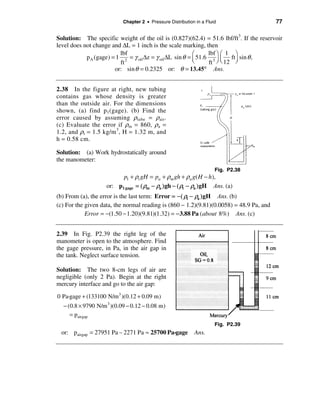
![78 Solutions Manual • Fluid Mechanics, Fifth Edition
2.40 In Fig. P2.40 the pressures at A and B are the same, 100 kPa. If water is
introduced at A to increase pA to 130 kPa, find and sketch the new positions of the
mercury menisci. The connecting tube is a uniform 1-cm in diameter. Assume no change
in the liquid densities.
Fig. P2.40
Solution: Since the tube diameter is constant, the volume of mercury will displace a
distance ∆h down the left side, equal to the volume increase on the right side; ∆h = ∆L. Apply
the hydrostatic relation to the pressure change, beginning at the right (air/mercury) interface:
p B + γ Hg (∆L sin θ + ∆h) − γ W (∆h + ∆L sin θ ) = p Α with ∆h = ∆L
or: 100,000 + 133100(∆h)(1 + sin15°) − 9790(∆h)(1 + sin15°) = p A = 130,000 Pa
Solve for ∆h = (30,000 Pa)/[(133100 – 9790 N/m 2 )(1 + sin15°)] = 0.193 m Ans.
The mercury in the left (vertical) leg will drop 19.3 cm, the mercury in the right (slanted)
leg will rise 19.3 cm along the slant and 0.05 cm in vertical elevation.
2.41 The system in Fig. P2.41 is at 20°C.
Determine the pressure at point A in
pounds per square foot.
Solution: Take the specific weights of
water and mercury from Table 2.1. Write
the hydrostatic formula from point A to the
water surface:
Fig. P2.41
æ 6 ö æ 10 ö æ 5ö lbf
p A + (0.85)(62.4 lbf/ft 3 ) ç ft ÷ − (846) ç ÷ + (62.4) ç ÷ = patm = (14.7)(144) 2
è 12 ø è 12 ø è 12 ø ft
Solve for p A = 2770 lbf/ft 2 Ans.](https://image.slidesharecdn.com/solucionariodefluidoswhite-120604143132-phpapp02/85/Solucionario-de-fluidos_white-78-320.jpg)
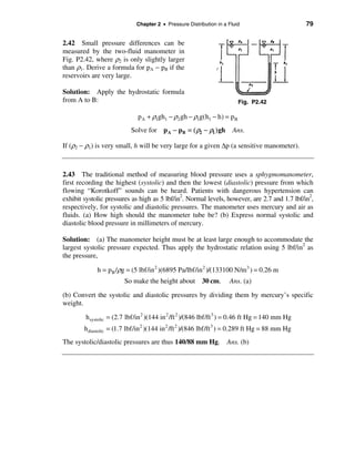

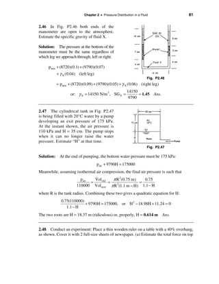
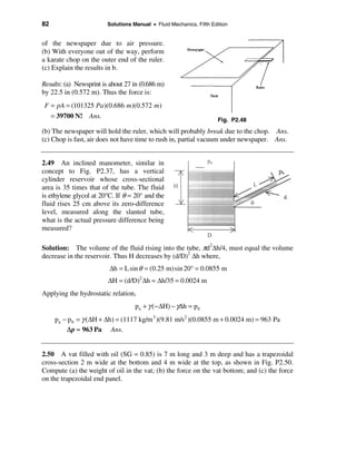

![84 Solutions Manual • Fluid Mechanics, Fifth Edition
2.52 A vertical lock gate is 4 m wide and separates 20°C water levels of 2 m and 3 m,
respectively. Find the moment about the bottom required to keep the gate stationary.
Solution: On the side of the gate where the water measures 3 m, F1 acts and has an hCG
of 1.5 m; on the opposite side, F2 acts with an hCG of 1 m.
F1 = γ h CG1A1 = (9790)(1.5)(3)(4) = 176,220 N
F2 = γ h CG2 A 2 = (9790)(1.0)(2)(4) = 78,320 N
y CP1 = [ −(1/12)(4)(3)3 sin 90°]/[(1.5)(4)(3)] = −0.5 m; so F1 acts at 1.5 – 0.5
= 1.0 m above B
y CP2 = [ −(1/12)(4)(2)3 sin 90°]/[(1)(4)(2)] = −0.333 m; F2 acts at 1.0 – 0.33
= 0.67 m above B
Taking moments about points B (see the figure),
å M B = (176,220 N)(1.0 m) – (78,320 N)(0.667 m)
= 124,000 N ⋅ m; M bottom = 124 kN ⋅ m.
2.53 Panel ABC in the slanted side of a
water tank (shown at right) is an isoceles
triangle with vertex at A and base BC = 2 m.
Find the water force on the panel and its
line of action.
Solution: (a) The centroid of ABC is 2/3
of the depth down, or 8/3 m from the
surface. The panel area is (1/2)(2 m)(5 m) =
5 m2. The water force is
FABC = γ h CG A panel = (9790)(2.67 m)(5 m 2 ) = 131, 000 N Ans. (a)](https://image.slidesharecdn.com/solucionariodefluidoswhite-120604143132-phpapp02/85/Solucionario-de-fluidos_white-84-320.jpg)
![Chapter 2 • Pressure Distribution in a Fluid 85
(b) The moment of inertia of ABC is (1/36)(2 m)(5 m)3 = 6.94 m4. From Eq. (2.44),
y CP = − I xx sin θ /(h CG A panel ) = −6.94 sin (53°)/[2.67(5)] = −0.417 m Ans. (b)
The center of pressure is 3.75 m down from A, or 1.25 m up from BC.
2.54 In Fig. P2.54, the hydrostatic force F is the same on the bottom of all three
containers, even though the weights of liquid above are quite different. The three bottom
shapes and the fluids are the same. This is called the hydrostatic paradox. Explain why it
is true and sketch a freebody of each of the liquid columns.
Fig. P2.54
Solution: The three freebodies are shown below. Pressure on the side-walls balances
the forces. In (a), downward side-pressure components help add to a light W. In (b) side
pressures are horizontal. In (c) upward side pressure helps reduce a heavy W.
2.55 Gate AB in Fig. P2.55 is 5 ft wide
into the paper, hinged at A, and restrained
by a stop at B. Compute (a) the force on
stop B; and (b) the reactions at A if h = 9.5 ft.
Solution: The centroid of AB is 2.0 ft
below A, hence the centroidal depth is
h + 2 − 4 = 7.5 ft. Then the total hydrostatic
force on the gate is Fig. P2.55
F = γ h CG A gate = (62.4 lbf/ft 3 )(7.5 ft)(20 ft 2 ) = 9360 lbf](https://image.slidesharecdn.com/solucionariodefluidoswhite-120604143132-phpapp02/85/Solucionario-de-fluidos_white-85-320.jpg)

 = 352,440 = 352 kN Ans. (b)
The resultant is the same as part (a): F = [(264)2 + (352)2]1/2 = 441 kN.
2.58 In Fig. P2.58, weightless cover gate
AB closes a circular opening 80 cm in
diameter when weighed down by the 200-kg
mass shown. What water level h will dislodge
the gate?
Solution: The centroidal depth is exactly Fig. P2.58
equal to h and force F will be upward on the gate. Dislodging occurs when F equals the
weight:
π
F = γ h CG A gate = (9790 N/m 3 ) h
(0.8 m)2 = W = (200)(9.81) N
4
Solve for h = 0.40 m Ans.
2.59 Gate AB has length L, width b into
the paper, is hinged at B, and has negligible
weight. The liquid level h remains at the
top of the gate for any angle θ. Find an
analytic expression for the force P, per-
pendicular to AB, required to keep the gate
in equilibrium.
Solution: The centroid of the gate remains
at distance L/2 from A and depth h/2 below](https://image.slidesharecdn.com/solucionariodefluidoswhite-120604143132-phpapp02/85/Solucionario-de-fluidos_white-87-320.jpg)
![88 Solutions Manual • Fluid Mechanics, Fifth Edition
the surface. For any θ, then, the hydrostatic force is F = γ (h/2)Lb. The moment of inertia
of the gate is (1/12)bL3, hence yCP = −(1/12)bL3sinθ/[(h/2)Lb], and the center of pressure
is (L/2 − yCP) from point B. Summing moments about hinge B yields
PL = F(L/2 − y CP ), or: P = (γ hb/4)( L − L2 sin θ /3h) Ans.
2.60 The pressure in the air gap is 8000 Pa
gage. The tank is cylindrical. Calculate the
net hydrostatic force (a) on the bottom of
the tank; (b) on the cylindrical sidewall
CC; and (c) on the annular plane panel BB.
Solution: (a) The bottom force is simply
equal to bottom pressure times bottom area:
p bottom = pair + ρwater g ∆z = 8000 Pa
+ (9790 N/m3 )(0.25 + 0.12 m)
Fig. P2.60
= 11622 Pa-gage
Fbottom = p bottom A bottom = (11622 Pa)(π /4)(0.36 m)2 = 1180 N Ans. (a)
(b) The net force on the cylindrical sidewall CC is zero due to symmetry. Ans. (b)
(c) The force on annular region CC is, like part (a), the pressure at CC times the area of CC:
pCC = pair + ρwater g ∆z CC = 8000 Pa + (9790 N/m 3 )(0.25 m) = 10448 Pa-gage
FCC = pCC A CC = (10448 Pa)(π /4)[(0.36 m)2 − (0.16 m)2 ] = 853 N Ans. (c)
2.61 Gate AB in Fig. P2.61 is a homo-
geneous mass of 180 kg, 1.2 m wide into
the paper, resting on smooth bottom B. All
fluids are at 20°C. For what water depth h
will the force at point B be zero?
Solution: Let γ = 12360 N/m3 for glycerin
and 9790 N/m3 for water. The centroid of
Fig. P2.61](https://image.slidesharecdn.com/solucionariodefluidoswhite-120604143132-phpapp02/85/Solucionario-de-fluidos_white-88-320.jpg)

![90 Solutions Manual • Fluid Mechanics, Fifth Edition
contributes to the hydrostatic force shown
in the freebody at right:
æ hö
F = γ h CG A = (62.4) ç ÷ (8h csc 60°)
è 2ø
= 288.2h 2 (lbf)
(1/12)(8)(h csc 60°)3sin 60°
y CP = −
(h/2)(8h csc 60°)
h
= − csc 60°
6
The weight of the gate is (7.85)(62.4 lbf/ft3)(15 ft)(1/12 ft)(8 ft) = 4898 lbf. This weight
acts downward at the CG of the full gate as shown (not the CG of the submerged
portion). Thus, W is 7.5 ft above point B and has moment arm (7.5 cos 60° ft) about B.
We are now in a position to find h by summing moments about the hinge line B:
å M B = (10000)(15) − (288.2h 2 )[(h/2)csc 60° − (h/6) csc 60°] − 4898(7.5cos 60°) = 0,
or: 110.9h3 = 150000 − 18369, h = (131631/110.9)1/3 = 10.6 ft Ans.
2.63 The tank in Fig. P2.63 has a 4-cm-
diameter plug which will pop out if the
hydrostatic force on it reaches 25 N. For
20°C fluids, what will be the reading h on
the manometer when this happens?
Solution: The water depth when the plug
pops out is
π (0.04)2
F = 25 N = γ h CG A = (9790)h CG Fig. P2.63
4
or h CG = 2.032 m
It makes little numerical difference, but the mercury-water interface is a little deeper than
this, by the amount (0.02 sin 50°) of plug-depth, plus 2 cm of tube length. Thus
patm + (9790)(2.032 + 0.02 sin 50° + 0.02) − (133100)h = patm ,
or: h ≈ 0.152 m Ans.](https://image.slidesharecdn.com/solucionariodefluidoswhite-120604143132-phpapp02/85/Solucionario-de-fluidos_white-90-320.jpg)


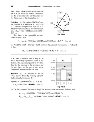
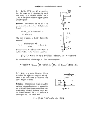
![96 Solutions Manual • Fluid Mechanics, Fifth Edition
Since the air pressure is uniform, Fair acts at the centroid of the gate, or 15 cm below the
hinge. The force imparted by the water is simply the hydrostatic force,
Fw = (γ h CG A)w = (9790 N/m 3 )(h − 0.15 m)(0.3 m)(0.6 m) = 1762.2h − 264.3
This force has a center of pressure at,
1
(0.6)(0.3)3 (sin90) 0.0075
y CP = 12 = with h in meters
(h − 0.15)(0.3)(0.6) h − 0.15
Sum moments about the hinge and set equal to zero to find the minimum height:
å M hinge = 0 = (1762.2h − 264.3)[0.15 + (0.0075/(h − 0.15))] − (1800)(0.15)
This is quadratic in h, but let’s simply solve by iteration: h = 1.12 m Ans.
2.73 Weightless gate AB is 5 ft wide into
the paper and opens to let fresh water out
when the ocean tide is falling. The hinge at
A is 2 ft above the freshwater level. Find h
when the gate opens.
Solution: There are two different hydro- Fig. P2.73
static forces and two different lines of
action. On the water side,
Fw = γ h CG A = (62.4)(5)(10 × 5) = 15600 lbf
positioned at 3.33 ft above point B. In the
seawater,
æ hö
Fs = (1.025 × 62.4) ç ÷ (5h)
è 2ø
= 159.9h (lbf)
2
positioned at h/3 above point B. Summing moments about hinge point A gives the
desired seawater depth h:
å M A = 0 = (159.9h 2 )(12 − h/3) − (15600)(12 − 3.33),
or 53.3h 3 − 1918.8h 2 + 135200 = 0, solve for h = 9.85 ft Ans.](https://image.slidesharecdn.com/solucionariodefluidoswhite-120604143132-phpapp02/85/Solucionario-de-fluidos_white-96-320.jpg)
![Chapter 2 • Pressure Distribution in a Fluid 97
2.74 Find the height H in Fig. P2.74 for
which the hydrostatic force on the rect-
angular panel is the same as the force on
the semicircular panel below. Find the
force on each panel and set them equal:
Frect = γ h CG A rect = γ (H/2)[(2R)(H)] = γ RH 2
Fsemi = γ h CG Asemi = γ (H + 4R/3π )[(π /2)R 2 ] Fig. P2.74
Set them equal, cancel γ : RH2 = (π /2)R2H + 2R3/3, or: H2 − (π /2)RH − 2R2/3 = 0
Solution: H = R[π /4 + {(π /4)2 + 2/3}1/2 ] ≈ 1.92R Ans.
2.75 Gate AB in the figure is hinged at A,
has width b into the paper, and makes
smooth contact at B. The gate has density
ρS and uniform thickness t. For what gate
density, expressed as a function of (h, t, ρ, θ),
will the gate just begin to lift off the
bottom? Why is your answer independent
of L and b?
Solution: Gate weight acts down at the
center between A and B. The hydrostatic Fig. P2.75
force acts at two-thirds of the way down the
gate from A. When “beginning to lift off,” there is no force at B. Summing moments
about A yields
L 2L h
W cosθ = F , F = ρ g bL, W = ρs gbLt
2 3 2
Combine and solve for the density of the gate. L and b and g drop out!
2h
ρs = ρ Ans.
3 t cosθ
2.76 Panel BC in Fig. P2.76 is circular. Compute (a) the hydrostatic force of the
water on the panel; (b) its center of pressure; and (c) the moment of this force about
point B.](https://image.slidesharecdn.com/solucionariodefluidoswhite-120604143132-phpapp02/85/Solucionario-de-fluidos_white-97-320.jpg)


![Chapter 2 • Pressure Distribution in a Fluid 101
On the right side, we have to write everything in terms of the centroidal depth hCG1 = h + 4 ft:
F1 = (62.4)(h CG1 )(70) = 4368h CG1
(1/12)(7)(10)3 sin(53.13°) 6.67
y CP1 = − =−
h CG1 (70) h CG1
Then we sum moments about B in the freebody above, taking FA = 0 (gate opening):
æ 6.67 ö
å M B = 0 = 4368h CG1 ç 5 − − 34944(5 − 0.833) − 3000(5cos 53.13°),
è h CG1 ÷
ø
183720
or: h CG1 = = 8.412 ft, or: h = h CG1 − 4 = 4.41 ft Ans.
21840
2.82 The dam in Fig. P2.82 is a quarter-
circle 50 m wide into the paper. Determine
the horizontal and vertical components of
hydrostatic force against the dam and the
point CP where the resultant strikes the dam. Fig. P2.82
Solution: The horizontal force acts as if
the dam were vertical and 20 m high:
FH = γ h CG A vert
= (9790 N/m 3 )(10 m)(20 × 50 m 2 )
= 97.9 MN Ans.
This force acts 2/3 of the way down or 13.33 m from the surface, as in the figure at right.
The vertical force is the weight of the fluid above the dam:
π
FV = γ (Vol)dam = (9790 N/m 3 ) (20 m)2 (50 m) = 153.8 MN Ans.
4
This vertical component acts through the centroid of the water above the dam, or 4R/3π =
4(20 m)/3π = 8.49 m to the right of point A, as shown in the figure. The resultant
hydrostatic force is F = [(97.9 MN)2 + (153.8 MN)2]1/2 = 182.3 MN acting down at an
angle of 32.5° from the vertical. The line of action of F strikes the circular-arc dam AB at
the center of pressure CP, which is 10.74 m to the right and 3.13 m up from point A, as
shown in the figure. Ans.](https://image.slidesharecdn.com/solucionariodefluidoswhite-120604143132-phpapp02/85/Solucionario-de-fluidos_white-101-320.jpg)
![Chapter 2 • Pressure Distribution in a Fluid 103
2.84 Determine (a) the total hydrostatic
force on curved surface AB in Fig. P2.84
and (b) its line of action. Neglect atmospheric
pressure and assume unit width into the
paper.
Solution: The horizontal force is
Fig. P2.84
FH = γ h CG A vert = (9790 N/m3 )(0.5 m)(1 × 1 m 2 ) = 4895 N at 0.667 m below B.
For the cubic-shaped surface AB, the weight
of water above is computed by integration:
1
3
FV = γ b ò (1 − x3 )dx = γ b
0
4
= (3/4)(9790)(1.0) = 7343 N
The line of action (water centroid) of the vertical force also has to be found by integration:
1
ò x(1 − x )dx
3
ò x dA 3/10
x= = 0
= = 0.4 m
ò dA 1
3/4
ò (1 − x ) dx
3
0
The vertical force of 7343 N thus acts at 0.4 m to the right of point A, or 0.6 m to the left
of B, as shown in the sketch above. The resultant hydrostatic force then is
Ftotal = [(4895)2 + (7343)2 ]1/2 = 8825 N acting at 56.31° down and to the right. Ans.
This result is shown in the sketch at above right. The line of action of F strikes the
vertical above point A at 0.933 m above A, or 0.067 m below the water surface.
2.85 Compute the horizontal and vertical
components of the hydrostatic force on the
quarter-circle panel at the bottom of the
water tank in Fig. P2.85.
Solution: The horizontal component is
FH = γ h CG A vert = (9790)(6)(2 × 6)
= 705000 N Ans. (a) Fig. P2.85](https://image.slidesharecdn.com/solucionariodefluidoswhite-120604143132-phpapp02/85/Solucionario-de-fluidos_white-103-320.jpg)
![104 Solutions Manual • Fluid Mechanics, Fifth Edition
The vertical component is the weight of the fluid above the quarter-circle panel:
FV = W(2 by 7 rectangle) − W(quarter-circle)
= (9790)(2 × 7 × 6) − (9790)(π /4)(2)2 (6)
= 822360 − 184537 = 638000 N Ans. (b)
2.86 The quarter circle gate BC in
Fig. P2.86 is hinged at C. Find the
horizontal force P required to hold the gate
stationary. The width b into the paper
is 3 m.
Solution: The horizontal component of Fig. P2.86
water force is
FH = γ h CG A = (9790 N/m 3 )(1 m)[(2 m)(3 m)] = 58,740 N
This force acts 2/3 of the way down or 1.333 m down from the surface (0.667 m
up from C). The vertical force is the weight of the quarter-circle of water above
gate BC:
FV = γ (Vol)water = (9790 N/m 3 )[(π /4)(2 m)2 (3 m)] = 92,270 N
F V acts down at (4R/3π) = 0.849 m to the left of C. Sum moments clockwise about
point C:
å MC = 0 = (2 m)P − (58740 N)(0.667 m) – (92270 N)(0.849 m) = 2P − 117480
Solve for P = 58,700 N = 58. 7 kN Ans.
2.87 The bottle of champagne (SG =
0.96) in Fig. P2.87 is under pressure as
shown by the mercury manometer reading.
Compute the net force on the 2-in-radius
hemispherical end cap at the bottom of the
bottle.
Solution: First, from the manometer, com-
pute the gage pressure at section AA in the
Fig. P2.87](https://image.slidesharecdn.com/solucionariodefluidoswhite-120604143132-phpapp02/85/Solucionario-de-fluidos_white-104-320.jpg)
![106 Solutions Manual • Fluid Mechanics, Fifth Edition
The net force is thus F = [FH + FV ]1/ 2 = 179100 N per meter of width, acting upward to
2 2
the right at an angle of 10.27° and passing through a point 1.0 m below and 0.4804 m
to the right of point B. This force passes, as expected, right through point O.
2.89 The tank in the figure contains
benzene and is pressurized to 200 kPa
(gage) in the air gap. Determine the vertical
hydrostatic force on circular-arc section AB
and its line of action.
Solution: Assume unit depth into the
paper. The vertical force is the weight of
benzene plus the force due to the air
pressure:
Fig. P2.89
π N
FV = (0.6)2 (1.0)(881)(9.81) + (200,000)(0.6)(1.0) = 122400 Ans.
4 m
Most of this (120,000 N/m) is due to the air pressure, whose line of action is in the
middle of the horizontal line through B. The vertical benzene force is 2400 N/m and has a
line of action (see Fig. 2.13 of the text) at 4R/(3π) = 25.5 cm to the right or A.
The moment of these two forces about A must equal to moment of the combined
(122,400 N/m) force times a distance X to the right of A:
(120000)(30 cm) + (2400)(25.5 cm) = 122400( X ), solve for X = 29.9 cm Ans.
The vertical force is 122400 N/m (down), acting at 29.9 cm to the right of A.
2.90 A 1-ft-diameter hole in the bottom
of the tank in Fig. P2.90 is closed by a
45° conical plug. Neglecting plug weight,
compute the force F required to keep the
plug in the hole.
Solution: The part of the cone that is
inside the water is 0.5 ft in radius and h =
0.5/tan(22.5°) = 1.207 ft high. The force F
Fig. P2.90
equals the air gage pressure times the hole](https://image.slidesharecdn.com/solucionariodefluidoswhite-120604143132-phpapp02/85/Solucionario-de-fluidos_white-106-320.jpg)

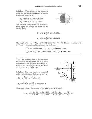
![110 Solutions Manual • Fluid Mechanics, Fifth Edition
−1
γs é2 h ù
Solve for: SGbody = = + Ans.
γ ê3 Rú
ë û
For h = 0, SG = 3/2 Ans. (a). For h = R, SG = 3/5 Ans. (b).
2.96 Curved panel BC is a 60° arc,
perpendicular to the bottom at C. If the
panel is 4 m wide into the paper, estimate
the resultant hydrostatic force of the water
on the panel.
Solution: The horizontal force is,
FH = γ h CG A h Fig. P2.96
= (9790 N/m )[2 + 0.5(3sin 60°) m]
3
× [(3sin 60°)m(4 m)]
= 335,650 N
The vertical component equals the weight
of water above the gate, which is the sum
of the rectangular piece above BC, and the
curvy triangular piece of water just above
arc BC—see figure at right. (The curvy-
triangle calculation is messy and is not
shown here.)
FV = γ (Vol)above BC = (9790 N/m 3 )[(3.0 + 1.133 m 2 )(4 m)] = 161,860 N
The resultant force is thus,
FR = [(335,650)2 + (161,860)2 ]1/2 = 372,635 N = 373 kN Ans.
This resultant force acts along a line which passes through point O at
θ = tan −1 (161,860/335,650) = 25.7°](https://image.slidesharecdn.com/solucionariodefluidoswhite-120604143132-phpapp02/85/Solucionario-de-fluidos_white-110-320.jpg)
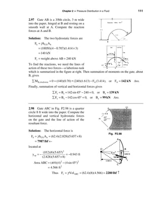
![112 Solutions Manual • Fluid Mechanics, Fifth Edition
The resultant is found to be
FR = [(7987)2 + (2280)2 ]1/2 = 8300 lbf acting at θ = 15.9° through the center O. Ans.
2.99 A 2-ft-diam sphere weighing 400 kbf
closes the 1-ft-diam hole in the tank
bottom. Find the force F to dislodge the
sphere from the hole.
Solution: NOTE: This problem is
laborious! Break up the system into regions
I,II,III,IV, & V. The respective volumes are:
Fig. P2.99
υ III = 0.0539 ft 3 ; υ II = 0.9419 ft 3
υ IV = υI = υ V = 1.3603 ft 3
Then the hydrostatic forces are:
Fdown = γυ II = (62.4)(0.9419) = 58.8 lbf
Fup = γ (υ I + υ V ) = (62.4)(2.7206)
= 169.8 lbf
Then the required force is F = W + Fdown − Fup = 400 + 59 − 170 = 289 lbf ↑ Ans.
2.100 Pressurized water fills the tank in
Fig. P2.100. Compute the hydrostatic force
on the conical surface ABC.
Solution: The gage pressure is equivalent
to a fictitious water level h = p/γ =
150000/9790 = 15.32 m above the gage or
8.32 m above AC. Then the vertical force
on the cone equals the weight of fictitious Fig. P2.100
water above ABC:
FV = γ Volabove
éπ 1π 2 ù
= (9790) ê (2)2 (8.32) + (2) (4)ú
ë4 34 û
= 297, 000 N Ans.](https://image.slidesharecdn.com/solucionariodefluidoswhite-120604143132-phpapp02/85/Solucionario-de-fluidos_white-112-320.jpg)
(2.356) = 25500 N
Then the total hydrostatic force on the end plate is 9050 + 25500 ≈ 34600 N Ans.
2.102 A cubical tank is 3 × 3 × 3 m and is layered with 1 meter of fluid of specific
gravity 1.0, 1 meter of fluid with SG = 0.9, and 1 meter of fluid with SG = 0.8. Neglect
atmospheric pressure. Find (a) the hydrostatic force on the bottom; and (b) the force on a
side panel.
Solution: (a) The force on the bottom is the bottom pressure times the bottom area:
Fbot = p bot A bot = (9790 N/m 3 )[(0.8 × 1 m) + (0.9 × 1 m) + (1.0 × 1 m)](3 m)2
= 238, 000 N Ans. (a)
(b) The hydrostatic force on the side panel is the sum of the forces due to each layer:
Fside = å γ h CG Aside = (0.8 × 9790 N/m 3 )(0.5 m)(3 m 2 ) + (0.9 × 9790 N/m 3 )(1.5 m)(3 m 2 )
+ (9790 N/m 3 )(2.5 m)(3 m 2 ) = 125, 000 kN Ans. (b)](https://image.slidesharecdn.com/solucionariodefluidoswhite-120604143132-phpapp02/85/Solucionario-de-fluidos_white-113-320.jpg)

![Chapter 2 • Pressure Distribution in a Fluid 115
Solution: The altitude can be determined by calculating the air density to provide the
proper buoyancy and then using Table A.3 to find the altitude associated with this density:
ρair = m balloon /Volsphere = (6.7 kg)/[π (2.5 m 3 )/6] = 0.819 kg/m 3
From Table A.3, atmospheric air has ρ = 0.819 kg/m3 at an altitude of about 4000 m. Ans.
2.107 Repeat Prob. 2.62 assuming that
the 10,000 lbf weight is aluminum (SG =
2.71) and is hanging submerged in the water.
Solution: Refer back to Prob. 2.62 for
details. The only difference is that the force
applied to gate AB by the weight is less
due to buoyancy:
(SG − 1) 2.71 − 1
Fnet = γυ body = (10000) = 6310 lbf
SG 2.71
This force replaces “10000” in the gate moment relation (see Prob. 2.62):
æh h ö
å M B = 0 = 6310(15) − (288.2h 2 ) ç csc 60° − csc 60°÷ − 4898(7.5cos 60°)
è2 6 ø
or: h 3 = 76280/110.9 = 688, or: h = 8.83 ft Ans.
2.108 A yellow pine rod (SG = 0.65) is
5 cm by 5 cm by 2.2 m long. How much
lead (SG = 11.4) is needed at one end so
that the rod will float vertically with 30 cm
out of the water?
Solution: The weight of wood and lead
must equal the buoyancy of immersed
wood and lead:
Wwood + Wlead = Bwood + Blead ,
or: (0.65)(9790)(0.05) (2.2) + 11.4(9790)υ lead = (9790)(0.05) (1.9) + 9790υlead
2 2
Solve for υ lead = 0.000113 m 3 whence Wlead = 11.4(9790)υ lead = 12.6 N Ans.](https://image.slidesharecdn.com/solucionariodefluidoswhite-120604143132-phpapp02/85/Solucionario-de-fluidos_white-115-320.jpg)
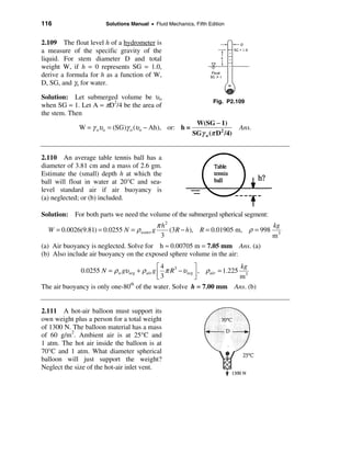


![120 Solutions Manual • Fluid Mechanics, Fifth Edition
2.117 The balloon in the figure is filled
with helium and pressurized to 135 kPa
and 20°C. The balloon material has a mass
of 85 g/m2. Estimate (a) the tension in the
mooring line, and (b) the height in the
standard atmosphere to which the balloon
will rise if the mooring line is cut. Fig. P2.117
Solution: (a) For helium, from Table A-4, R = 2077 m2/s2/K, hence its weight is
é 135000 ù éπ 3ù
Whelium = ρ He gυballoon = ê ú (9.81) ê 6 (10) ú = 1139 N
ë 2077(293) û ë û
Meanwhile, the total weight of the balloon material is
æ kg ö æ mö
Wballoon = ç 0.085 2 ÷ ç 9.81 2 ÷ [π (10 m)2 ] = 262 N
è m øè s ø
Finally, the balloon buoyancy is the weight of displaced air:
é 100000 ù éπ 3ù
Bair = ρair gυballoon = ê ú (9.81) ê 6 (10) ú = 6108 N
ë 287(293) û ë û
The difference between these is the tension in the mooring line:
Tline = Bair − Whelium − Wballoon = 6108 − 1139 − 262 ≈ 4700 N Ans. (a)
(b) If released, and the balloon remains at 135 kPa and 20°C, equilibrium occurs when
the balloon air buoyancy exactly equals the total weight of 1139 + 262 = 1401 N:
π kg
Bair = 1401 N = ρ air (9.81) (10)3 , or: ρ air ≈ 0.273 3
6 m
From Table A-6, this standard density occurs at approximately
Z ≈ 12, 800 m Ans. (b)
2.118 A 14-in-diameter hollow sphere of
steel (SG = 7.85) has 0.16 in wall thickness.
How high will this sphere float in 20°C
water? How much weight must be added
inside to make the sphere neutrally
buoyant?](https://image.slidesharecdn.com/solucionariodefluidoswhite-120604143132-phpapp02/85/Solucionario-de-fluidos_white-120-320.jpg)
![Chapter 2 • Pressure Distribution in a Fluid 121
Solution: The weight of the steel is
π éæ 14 ö æ 13.68 ö ù
3 3
Wsteel = γ Vol = (7.85)(62.4) êç ÷ − ç ÷ ú
6 êè 12 ø è 12 ø ú
ë û
= 27.3 lbf
This is equivalent to 27.3/62.4 = 0.437 ft3 of displaced water, whereas υsphere = 0.831 ft3.
Therefore the sphere floats slightly above its midline, such that the sphere segment
volume, of height h in the figure, equals the displaced volume:
π 2 π
υsegment = 0.437 ft 3 = h (3R − h) = h 2 [3(7/12) − h]
3 3
Solve for h = 0.604 ft ≈ 7.24 in Ans.
In order for the sphere to be neutrally buoyant, we need another (0.831 − 0.437) = 0.394 ft3
of displaced water, so we need additional weight ∆W = 62.4(0.394) ≈ 25 lbf. Ans.
2.119 With a 5-lbf-weight placed at one
end, the uniform wooden beam in the
figure floats at an angle θ with its upper
right corner at the surface. Determine (a) θ;
(b) γwood. Fig. P2.119
Solution: The total wood volume is (4/12)2(9) = 1 ft3. The exposed distance h = 9tanθ.
The vertical forces are
å Fz = 0 = (62.4)(1.0) − (62.4)(h/2)(9)(4/12) − (SG)(62.4)(1.0) − 5 lbf
The moments of these forces about point C at the right corner are:
å MC = 0 = γ (1)(4.5) − γ (1.5h)(6 ft) − (SG)(γ )(1)(4.5 ft) + (5 lbf)(0 ft)
where γ = 62.4 lbf/ft3 is the specific weight of water. Clean these two equations up:
1.5h = 1 − SG − 5/γ (forces) 2.0h = 1 − SG (moments)
Solve simultaneously for SG ≈ 0.68 Ans. (b); h = 0.16 ft; θ ≈ 1.02° Ans. (a)](https://image.slidesharecdn.com/solucionariodefluidoswhite-120604143132-phpapp02/85/Solucionario-de-fluidos_white-121-320.jpg)
![122 Solutions Manual • Fluid Mechanics, Fifth Edition
2.120 A uniform wooden beam (SG =
0.65) is 10 cm by 10 cm by 3 m and hinged
at A. At what angle will the beam float in
20°C water?
Solution: The total beam volume is
3(.1)2 = 0.03 m3, and therefore its weight is
W = (0.65)(9790)(0.03) = 190.9 N, acting
at the centroid, 1.5 m down from point A.
Meanwhile, if the submerged length is H, Fig. P2.120
the buoyancy is B = (9790)(0.1)2H = 97.9H
newtons, acting at H/2 from the lower end.
Sum moments about point A:
å M A = 0 = (97.9H)(3.0 − H/2) cos θ − 190.9(1.5cos θ ),
or: H(3 − H/2) = 2.925, solve for H ≈ 1.225 m
Geometry: 3 − H = 1.775 m is out of the water, or: sinθ = 1.0/1.775, or θ ≈ 34.3° Ans.
2.121 The uniform beam in the figure is of
size L by h by b, with b,h = L. A uniform
heavy sphere tied to the left corner causes
the beam to float exactly on its diagonal.
Show that this condition requires (a) γ b =
γ /3; and (b) D = [Lhb/{π(SG − 1)}]1/3.
Solution: The beam weight W = γ bLhb
and acts in the center, at L/2 from the left
corner, while the buoyancy, being a perfect Fig. P2.121
triangle of displaced water, equals B =
γ Lhb/2 and acts at L/3 from the left corner.
Sum moments about the left corner, point C:
å MC = 0 = (γ b Lhb)(L/2) − (γ Lhb/2)(L/3), or: γ b = γ /3 Ans. (a)
Then summing vertical forces gives the required string tension T on the left corner:
å Fz = 0 = γ Lbh/2 − γ b Lbh − T, or T = γ Lbh/6 since γ b = γ /3
1/3
π é Lhb ù
But also T = (W − B)sphere = (SG − 1)γ D3 , so that D = ê ú Ans. (b)
6 ë π (SG − 1) û](https://image.slidesharecdn.com/solucionariodefluidoswhite-120604143132-phpapp02/85/Solucionario-de-fluidos_white-122-320.jpg)
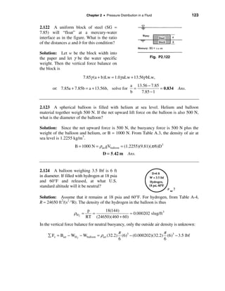
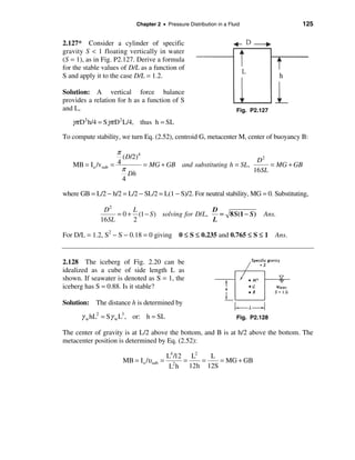
![126 Solutions Manual • Fluid Mechanics, Fifth Edition
Noting that GB = L/2 − h/2 = L(1 − S)/2, we may solve for the metacentric height:
L L 1
MG = − (1 − S) = 0 if S2 − S + = 0, or: S = 0.211 or 0.789
12S 2 6
Instability: 0.211 < S < 0.789. Since the iceberg has S = 0.88 > 0.789, it is stable. Ans.
2.129 The iceberg of Prob. 2.128 may
become unstable if its width decreases.
Suppose that the height is L and the depth
into the paper is L but the width decreases
to H < L. Again with S = 0.88 for the
iceberg, determine the ratio H/L for which
the iceberg becomes unstable.
Solution: As in Prob. 2.128, the submerged distance h = SL = 0.88L, with G at L/2
above the bottom and B at h/2 above the bottom. From Eq. (2.52), the distance MB is
Io LH3 /12 H2 æ L SL ö
MB = = = = MG + GB = MG + ç −
υsub HL(SL) 12SL è2 2 ÷ ø
Then neutral stability occurs when MG = 0, or
H2 L H
= (1 − S), or = [6S(1 − S)]1/2 = [6(0.88)(1 − 0.88)]1/2 = 0.796 Ans.
12SL 2 L
2.130 Consider a wooden cylinder (SG =
0.6) 1 m in diameter and 0.8 m long.
Would this cylinder be stable if placed to
float with its axis vertical in oil (SG = 0.85)?
Solution: A vertical force balance gives
0.85π R 2 h = 0.6π R 2 (0.8 m),
or: h = 0.565 m
The point B is at h/2 = 0.282 m above the bottom. Use Eq. (2.52) to predict the meta-
center location:
MB = I o /υsub = [π (0.5)4 /4] /[π (0.5)2 (0.565)] = 0.111 m = MG + GB](https://image.slidesharecdn.com/solucionariodefluidoswhite-120604143132-phpapp02/85/Solucionario-de-fluidos_white-126-320.jpg)

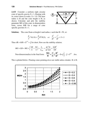
![Chapter 2 • Pressure Distribution in a Fluid 129
2.134 When floating in water (SG = 1),
an equilateral triangular body (SG = 0.9)
might take two positions, as shown at right.
Which position is more stable? Assume
large body width into the paper.
Fig. P2.134
Solution: The calculations are similar to the floating cone of Prob. 2.132. Let the
triangle be L by L by L. List the basic results.
(a) Floating with point up: Centroid G is 0.289L above the bottom line, center of buoyancy B
is 0.245L above the bottom, hence GB = (0.289 − 0.245)L ≈ 0.044L. Equation (2.52) gives
MB = I o /υsub = 0.0068L = MG + GB = MG + 0.044L
Hence MG = −0.037L Unstable Ans. (a)
(b) Floating with point down: Centroid G is 0.577L above the bottom point, center of
buoyancy B is 0.548L above the bottom point, hence GB = (0.577 − 0.548)L ≈ 0.0296L.
Equation (2.52) gives
MB = I o /υsub = 0.1826L = MG + GB = MG + 0.0296L
Hence MG = +0.153L Stable Ans. (b)
2.135 Consider a homogeneous right
circular cylinder of length L, radius R, and
specific gravity SG, floating in water (SG = 1)
with its axis vertical. Show that the body is
stable if
R/L > [2SG(1 − SG)]1/2
Solution: For a given SG, the body floats
with a draft equal to (SG)L, as shown. Its
center of gravity G is at L/2 above the
bottom. Its center of buoyancy B is at
(SG)L/2 above the bottom. Then Eq. (2.52)
predicts the metacenter location:
π R 4 /4 R2 L L
MB = I o /υsub = = = MG + GB = MG + − SG
π R (SG)L 4(SG)L
2
2 2
Thus MG > 0 (stability) if R 2 /L2 > 2SG(1 − SG) Ans.
For example, if SG = 0.8, stability requires that R/L > 0.566.](https://image.slidesharecdn.com/solucionariodefluidoswhite-120604143132-phpapp02/85/Solucionario-de-fluidos_white-129-320.jpg)
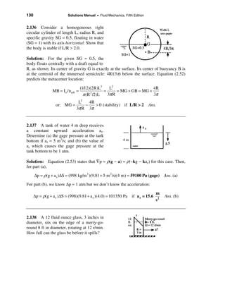
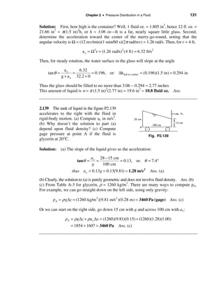
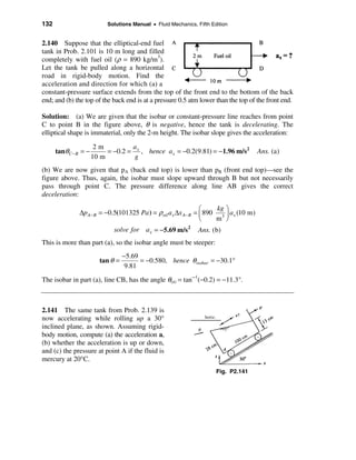
![Chapter 2 • Pressure Distribution in a Fluid 133
Solution: The free surface is tilted at the angle θ = −30° + 7.41° = −22.59°. This angle
must satisfy Eq. (2.55):
tan θ = tan(−22.59°) = −0.416 = a x /(g + a z )
But the 30° incline constrains the acceleration such that ax = 0.866a, az = 0.5a. Thus
0.866a m
tan θ = −0.416 = , solve for a ≈ − 3.80 2 (down) Ans. (a, b)
9.81 + 0.5a s
The cartesian components are aX = −3.29 m/s2 and aZ = −1.90 m/s2.
(c) The distance ∆S normal from the surface down to point A is (28 cosθ) cm. Thus
p A = ρ[a 2 + (g + a z )2 ]1/2 = (13550)[(−3.29)2 + (9.81 − 1.90)2 ]1/2 (0.28 cos 7.41°)
x
≈ 32200 Pa (gage) Ans. (c)
2.142 The tank of water in Fig. P2.142 is
12 cm wide into the paper. If the tank is
accelerated to the right in rigid-body
motion at 6 m/s2, compute (a) the water
depth at AB, and (b) the water force on
panel AB.
Solution: From Eq. (2.55),
Fig. P2.142
6.0
tan θ = a x /g = = 0.612, or θ ≈ 31.45°
9.81
Then surface point B on the left rises an additional ∆z = 12 tanθ ≈ 7.34 cm,
or: water depth AB = 9 + 7.34 ≈ 16.3 cm Ans. (a)
The water pressure on AB varies linearly due to gravity only, thus the water force is
æ 0.163 ö
FAB = p CG A AB = (9790) ç m÷ (0.163 m)(0.12 m) ≈ 15.7 N Ans. (b)
è 2 ø](https://image.slidesharecdn.com/solucionariodefluidoswhite-120604143132-phpapp02/85/Solucionario-de-fluidos_white-133-320.jpg)
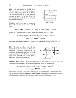

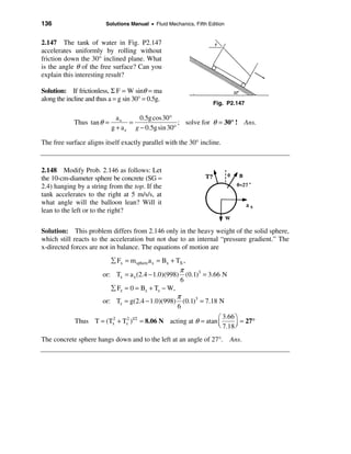


![Chapter 2 • Pressure Distribution in a Fluid 139
Solution: Convert Ω = 150 r/min = 15.7 rad/s. (a) The parabolic surfaces which result
are entirely independent of the fluid density, hence both interfaces will curl up into the
same-shape paraboloid, with a deflection ∆h up at the wall and down in the center:
Ω2 R 2 (15.7)2 (0.09)2
∆h = = = 0.051 m = 5.1 cm Ans. (a)
4g 4(9.81)
(b) The fluid pressure will be highest at point B in the bottom corner. We can compute
this by moving straight down through the oil and water at the wall, with gravity only:
p B = ρoil g∆z oil + ρwater g∆z water
= (891)(9.81)(0.1 m) + (998)(9.81)(0.051 + 0.12 m) = 2550 Pa (gage) Ans. (b)
2.155 For what uniform rotation rate in
r/min about axis C will the U-tube fluid in
Fig. P2.155 take the position shown? The
fluid is mercury at 20°C.
Solution: Let ho be the height of the
free surface at the centerline. Then, from
Eq. (2.64),
Fig. P2.155
Ω2 R 2 Ω2 R 2
zB = ho + B
; zA = ho + A
; R B = 0.05 m and R A = 0.1 m
2g 2g
Ω2
Subtract: z A − z B = 0.08 m = [(0.1)2 − (0.05)2 ],
2(9.81)
rad r
solve Ω = 14.5 = 138 Ans.
s min
The fact that the fluid is mercury does not enter into this “kinematic” calculation.
2.156 Suppose the U-tube of Prob. 2.151
is rotated about axis DC. If the fluid is
water at 122°F and atmospheric pressure is
2116 psfa, at what rotation rate will the
fluid begin to vaporize? At what point in
the tube will this happen?](https://image.slidesharecdn.com/solucionariodefluidoswhite-120604143132-phpapp02/85/Solucionario-de-fluidos_white-139-320.jpg)

![Chapter 2 • Pressure Distribution in a Fluid 141
2.158* It is desired to make a 3-m-
diameter parabolic telescope mirror by
rotating molten glass in rigid-body motion
until the desired shape is achieved and then
cooling the glass to a solid. The focus of
the mirror is to be 4 m from the mirror,
measured along the centerline. What is the
proper mirror rotation rate, in rev/min?
Solution: We have to review our math book, or Mark’s Manual, to recall that the focus F
of a parabola is the point for which all points on the parabola are equidistant from both
the focus and a so-called “directrix” line (which is one focal length below the mirror).
For the focal length h and the z-r axes shown in the figure, the equation of the parabola is
given by r2 = 4hz, with h = 4 m for our example.
Meanwhile the equation of the free-surface of the liquid is given by z = r2Ω2/(2g).
Set these two equal to find the proper rotation rate:
r 2 Ω2 r 2 g 9.81
z= = , or: Ω 2 = = = 1.226
2g 4h 2h 2(4)
rad æ 60 ö
Thus Ω = 1.107 ç ÷ = 10.6 rev/min Ans.
s è 2π ø
The focal point F is far above the mirror itself. If we put in r = 1.5 m and calculate the
mirror depth “L” shown in the figure, we get L ≈ 14 centimeters.
2.159 The three-legged manometer in
Fig. P2.159 is filled with water to a depth
of 20 cm. All tubes are long and have equal
small diameters. If the system spins at
angular velocity Ω about the central tube,
(a) derive a formula to find the change of
height in the tubes; (b) find the height in
cm in each tube if Ω = 120 rev/min. [HINT:
The central tube must supply water to both Fig. P2.159
the outer legs.]
Solution: (a) The free-surface during rotation is visualized as the red dashed line in
Fig. P2.159. The outer right and left legs experience an increase which is one-half that
of the central leg, or ∆hO = ∆hC/2. The total displacement between outer and center
menisci is, from Eq. (2.64) and Fig. 2.23, equal to Ω 2R2/(2g). The center meniscus](https://image.slidesharecdn.com/solucionariodefluidoswhite-120604143132-phpapp02/85/Solucionario-de-fluidos_white-141-320.jpg)


![144 Solutions Manual • Fluid Mechanics, Fifth Edition
COMPREHENSIVE PROBLEMS
C2.1 Some manometers are constructed as in the figure at
right, with one large reservoir and one small tube open to the
atmosphere. We can then neglect movement of the reservoir
level. If the reservoir is not large, its level will move, as in
the figure. Tube height h is measured from the zero-pressure
level, as shown.
(a) Let the reservoir pressure be high, as in the Figure, so its level
goes down. Write an exact Expression for p1gage as a function of
h, d, D, and gravity g. (b) Write an approximate expression for p1gage, neglecting the movement
of the reservoir. (c) Suppose h = 26 cm, pa = 101 kPa, and ρm = 820 kg/m3. Estimate the ratio
(D/d) required to keep the error in (b) less than 1.0% and also < 0.1%. Neglect surface tension.
Solution: Let H be the downward movement of the reservoir. If we neglect air density,
the pressure difference is p1 − pa = ρmg(h + H). But volumes of liquid must balance:
π 2 π
D H = d 2 h, or: H = (d /D)2 h
4 4
Then the pressure difference (exact except for air density) becomes
p1 − pa = p1 gage = ρm gh(1 + d 2 / D2 ) Ans. (a)
If we ignore the displacement H, then p1gage ≈ ρmgh Ans. (b)
(c) For the given numerical values, h = 26 cm and ρm = 820 kg/m3 are irrelevant, all that
matters is the ratio d/D. That is,
∆pexact − ∆papprox ( d /D ) 2
Error E = = , or : D/d = (1 − E )/E
∆pexact 1 + (d /D)2
For E = 1% or 0.01, D/d = [(1 − 0.01)/0.01]1/2 ≥ 9.95 Ans. (c-1%)
For E = 0.1% or 0.001, D/d = [(1 − 0.001)/0.001]1/2 ≥ 31.6 Ans. (c-0.1%)
C2.2 A prankster has added oil, of specific gravity SGo,
to the left leg of the manometer at right. Nevertheless, the
U-tube is still to be used to measure the pressure in the
air tank. (a) Find an expression for h as a function of H
and other parameters in the problem.
(b) Find the special case of your result when ptank = pa.
(c) Suppose H = 5 cm, pa = 101.2 kPa, SGo = 0.85, and
ptank is 1.82 kPa higher than pa. Calculate h in cm,
ignoring surface tension and air density effects.](https://image.slidesharecdn.com/solucionariodefluidoswhite-120604143132-phpapp02/85/Solucionario-de-fluidos_white-144-320.jpg)
![Chapter 2 • Pressure Distribution in a Fluid 145
Solution: Equate pressures at level i in the tube:
p i = pa + ρgH + ρw g(h − H) = p tank ,
ρ = SG o ρw (ignore the column of air in the right leg)
ptk − pa
Solve for: h = + H (1 − SGo ) Ans. (a)
ρw g
If ptank = pa, then
h = H (1 − SGo ) Ans. (b)
(c) For the particular numerical values given above, the answer to (a) becomes
1820 Pa
h= + 0.05(1 − 0.85) = 0.186 + 0.0075 = 0.193 m = 19.3 cm Ans. (c)
998(9.81)
Note that this result is not affected by the actual value of atmospheric pressure.
C2.3 Professor F. Dynamics, riding the merry-go-round with his son, has brought along
his U-tube manometer. (You never know when a manometer might come in handy.) As
shown in Fig. C2.2, the merry-go-round spins at constant angular velocity and the manometer
legs are 7 cm apart. The manometer center is 5.8 m from the axis of rotation. Determine
the height difference h in two ways: (a) approximately, by assuming rigid body
translation with a equal to the average manometer acceleration; and (b) exactly, using
rigid-body rotation theory. How good is the approximation?
Solution: (a) Approximate: The average acceleration of
the manometer is RavgΩ2 = 5.8[6(2π /60)]2 = 2.29 rad/s
toward the center of rotation, as shown. Then
tan(θ ) = a/g = 2.29/9.81 = h/(7 cm) = 0.233
Solve for h = 1.63 cm Ans. (a)](https://image.slidesharecdn.com/solucionariodefluidoswhite-120604143132-phpapp02/85/Solucionario-de-fluidos_white-145-320.jpg)
![146 Solutions Manual • Fluid Mechanics, Fifth Edition
(b) Exact: The isobar in the figure at right would be on the parabola z = C + r2Ω2/(2g),
where C is a constant. Apply this to the left leg (z1) and right leg (z2). As above, the
rotation rate is Ω = 6.0*(2π /60) = 0.6283 rad/s. Then
Ω2 2 2 (0.6283)2
h = z2 − z1 = (r2 − r1 ) = [(5.8 + 0.035)2 − (5.8 − 0.035)2 ]
2g 2(9.81)
= 0.0163 m Ans. (b)
This is nearly identical to the approximate answer (a), because R ? ∆r.
C2.4 A student sneaks a glass of cola onto a roller coaster ride. The glass is cylindrical,
twice as tall as it is wide, and filled to the brim. He wants to know what percent of the cola
he should drink before the ride begins, so that none of it spills during the big drop, in which
the roller coaster achieves 0.55-g acceleration at a 45° angle below the horizontal. Make the
calculation for him, neglecting sloshing and assuming that the glass is vertical at all times.
Solution: We have both horizontal and ver-
tical acceleration. Thus the angle of tilt α is
ax 0.55g cos 45°
tan α = = = 0.6364
g + az g − 0.55g sin 45°
Thus α = 32.47°. The tilted surface strikes the
centerline at Rtanα = 0.6364R below the top.
So the student should drink the cola until its
rest position is 0.6364R below the top. The
percentage drop in liquid level (and therefore
liquid volume) is
0.6364 R
% removed = = 0.159 or: 15.9% Ans.
4R
C2.5 Dry adiabatic lapse rate is defined as DALR = –dT/dz when T and p vary
isentropically. Assuming T = Cpa, where a = (γ – 1)/γ, γ = cp/cv, (a) show that DALR =
g(γ – 1)/(γ R), R = gas constant; and (b) calculate DALR for air in units of °C/km.
Solution: Write T(p) in the form T/To = (p/po)a and differentiate:
a −1
dT æ pö 1 dp dp
= To a ç ÷ , But for the hydrostatic condition: = −ρg
dz è po ø po dz dz](https://image.slidesharecdn.com/solucionariodefluidoswhite-120604143132-phpapp02/85/Solucionario-de-fluidos_white-146-320.jpg)
![Chapter 2 • Pressure Distribution in a Fluid 147
Substitute ρ = p/RT for an ideal gas, combine above, and rewrite:
a −1 a a
dT T æ pö p ag æ T ö æ p ö T æ pö
=− o aç ÷ g = − ç o ÷ ç ÷ . But: o ç ÷ = 1 (isentropic)
dz po è po ø RT R è T ø è po ø T è po ø
Therefore, finally,
dT ag (γ − 1)g
− = DALR = = Ans. (a)
dz R γR
(b) Regardless of the actual air temperature and pressure, the DALR for air equals
|s = (1.4 − 1)(9.81 2m/s ) = 0.00977 °C = 9.77 °C
2
dT
DALR = − Ans. (b)
dz 1.4(287 m 2 /s /°C ) m km
C2.6 Use the approximate pressure-density relation for a “soft” liquid,
dp = a 2 dρ, or p = p o + a 2 (ρ − ρo )
to derive a formula for the density distribution ρ(z) and pressure distribution p(z) in a
column of soft liquid. Then find the force F on a vertical wall of width b, extending from
z = 0 down to z = −h, and compare with the incompressible result F = ρogh2b/2.
Solution: Introduce this p(ρ) relation into the hydrostatic relation (2.18) and integrate:
ρ
dρ
z
g dz 2
dp = a dρ = −γ dz = − ρ g dz, or: ò
2
= − ò 2 , or: ρ = ρo e − gz/a Ans.
ρo
ρ 0 a
assuming constant a2. Substitute into the p(ρ) relation to obtain the pressure distribution:
2
p ≈ po + a 2 ρo [e − gz/a − 1] (1)
Since p(z) increases with z at a greater than linear rate, the center of pressure will always
be a little lower than predicted by linear theory (Eq. 2.44). Integrate Eq. (1) above,
neglecting po, into the pressure force on a vertical plate extending from z = 0 to z = −h:
−h 0
2 é a2 2 ù
F = − ò pb dz = ò a 2 ρo (e − gz/a − 1)b dz = ba 2 ρo ê ( e gh/a − 1) − h ú Ans.
0 −h ëg û
In the limit of small depth change relative to the “softness” of the liquid, h = a 2 /g, this
reduces to the linear formula F = ρogh2b/2 by expanding the exponential into the first
three terms of its series. For “hard” liquids, the difference in the two formulas is
negligible. For example, for water (a ≈ 1490 m/s) with h = 10 m and b = 1 m, the linear
formula predicts F = 489500 N while the exponential formula predicts F = 489507 N.](https://image.slidesharecdn.com/solucionariodefluidoswhite-120604143132-phpapp02/85/Solucionario-de-fluidos_white-147-320.jpg)

![150 Solutions Manual • Fluid Mechanics, Fifth Edition
data for 1.75 < r < 2.0 cm.) The volume flow, Q = ò u(2π r)dr, can be estimated by a
numerical quadrature formula such as Simpson’s rule. Here there are nine data points:
æ ∆r ö
Q = 2π (r1u1 + 4r2u2 + 2r3u3 + 4r4u4 + 2r5u5 + 4r6u6 + 2r7u7 + 4r8u8 + r9u9 ) ç ÷
è 3 ø
For the given data, Q ≈ 0.0059 m 3 /s Ans.
3.6 When a gravity-driven liquid jet
issues from a slot in a tank, as in Fig. P3.6,
an approximation for the exit velocity
distribution is u ≈ 2g(h − z), where h is
the depth of the jet centerline. Near the
slot, the jet is horizontal, two-dimensional,
and of thickness 2L, as shown. Find a
general expression for the total volume
flow Q issuing from the slot; then take the Fig. P3.6
limit of your result if L = h.
Solution: Let the slot width be b into the paper. Then the volume flow from Eq. (3.7) is
+L
2b
Q = ò u dA = ò [2g(h − z)]1/2 b dz = √(2g)[(h + L)3/2 − (h − L)3/2 ] Ans.
−L
3
In the limit of L = h, this formula reduces to Q ≈ (2Lb) (2gh) Ans.
3.7 In Chap. 8 a theory gives the velocities for flow past a cylinder:
v r = U cosθ (1 − R 2 /r 2 )
vθ = − U sinθ (1 + R 2 /r 2 )
Compute the volume flow Q passing through surface CC in the figure.
Fig. P3.7](https://image.slidesharecdn.com/solucionariodefluidoswhite-120604143132-phpapp02/85/Solucionario-de-fluidos_white-150-320.jpg)
![Chapter 3 • Integral Relations for a Control Volume 151
Solution: This problem is quite laborious and illustrates the difficulty of working with
polar velocity components passing through a cartesian (plane) surface. From Eq. (3.7),
+R
Q = ò (V ⋅ n) dA = ò (vr cosθ − vθ sinθ )b dy, where y = r sinθ
−R
We have to integrate over surface CC, where r varies from 2R to 2.24R and θ varies from
153.4° to 206.6°. Inserting the velocity components as given we obtain
+R
Q= ò [U cos2θ (1 − R 2 /r 2 ) + U sin 2θ (1 + R 2 /r 2 )]b dy |x =−2R = 1.6URb Ans.
−R
The integration is messy. In Chaps. 4&8 we find the result easily using the stream function.
3.8 Three pipes steadily deliver water at
20°C to a large exit pipe in Fig. P3.8. The
velocity V2 = 5 m/s, and the exit flow rate
Q4 = 120 m3/h. Find (a) V1; (b) V3; and
(c) V4 if it is known that increasing Q3 by
20% would increase Q4 by 10%.
Solution: (a) For steady flow we have
Q1 + Q2 + Q3 = Q4, or Fig. P3.8
V1 A1 + V2 A2 + V3 A3 = V4 A4 (1)
Since 0.2Q3 = 0.1Q4, and Q4 = (120 m3/h)(h/3600 s) = 0.0333 m3/s,
Q4 (0.0333 m 3 /s)
V3 = = = 5.89 m/s Ans. (b)
2 A3 π 2
(0.06 )
2
Substituting into (1),
æπ ö æπ ö æπ ö
V1 ç ÷ (0.04 2 ) + (5) ç ÷ (0.052 ) + (5.89) ç ÷ (0.06 2 ) = 0.0333 V1 = 5.45 m/s Ans. (a)
è4ø è4ø è4ø
From mass conservation, Q4 = V4A4
(0.0333 m 3 /s) = V4 (π )(0.06 2 )/4 V4 = 5.24 m/s Ans. (c)](https://image.slidesharecdn.com/solucionariodefluidoswhite-120604143132-phpapp02/85/Solucionario-de-fluidos_white-151-320.jpg)

![158 Solutions Manual • Fluid Mechanics, Fifth Edition
Solution: Recall that “relative humidity” is the ratio of water-vapor density present in
the air to the saturated vapor density at the same temperature. From Tables A-4 and A-5
for water at 30°C, Rgas = 461 J/(kg · °K) and pvap = 4242 Pa. Then, at 100% humidity,
pvap 4242
ρvapor = = = 0.0304 kg/m 3
RT (461)(303)
Meanwhile, the inlet volume flow of wet air is Qin = AV = (π/4)(0.08 m)2(3 m/s) = 0.0151 m3/s.
It follows that the mass of water vapor entering is ρvapQin = 4.58E−4 kg/s. If the air leaves
at 50% relative humidity, exactly half of this is drained away:
kg
&
m drained away = (1/2)(4.58E − 4)(3600) ≈ 0.82 Ans.
hr
3.22 The converging-diverging nozzle
shown in Fig. P3.22 expands and accelerates
dry air to supersonic speeds at the exit, where
p2 = 8 kPa and T2 = 240 K. At the throat,
p1 = 284 kPa, T1 = 665 K, and V1 = 517 m/s.
For steady compressible flow of an ideal gas,
estimate (a) the mass flow in kg/h, (b) the
velocity V2, and (c) the Mach number Ma2. Fig. P3.22
Solution: The mass flow is given by the throat conditions:
é 284000 kg ù π æ mö kg
m = ρ1A1V1 = ê
& 3ú
(0.01 m)2 ç 517 ÷ = 0.0604 Ans. (a)
ë (287)(665) m û 4 è sø s
For steady flow, this must equal the mass flow at the exit:
kg é 8000 ù π m
0.0604 = ρ2 A 2 V2 = ê ú 4 (0.025) V2, or V2 ≈ 1060 s
2
Ans. (b)
s ë 287(240) û
Recall from Eq. (1.39) that the speed of sound of an ideal gas = (kRT)1/2. Then
1060
Mach number at exit: Ma = V2 /a 2 = ≈ 3.41 Ans. (c)
[1.4(287)(240)]1/2
3.23 The hypodermic needle in the figure contains a liquid (SG = 1.05). If the serum is
to be injected steadily at 6 cm3/s, how fast should the plunger be advanced (a) if leakage
in the plunger clearance is neglected; and (b) if leakage is 10 percent of the needle flow?](https://image.slidesharecdn.com/solucionariodefluidoswhite-120604143132-phpapp02/85/Solucionario-de-fluidos_white-158-320.jpg)

![Chapter 3 • Integral Relations for a Control Volume 161
3.27 The cone frustum in the figure
contains incompressible liquid to depth h.
A solid piston of diameter d penetrates the
surface at velocity V. Derive an analytic
expression for the rate of rise dh/dt of the
liquid surface.
Solution: The piston motion is equivalent to a volume flow Qin = VApiston into the
liquid. A control volume around the frustum tank yields
d ìπ π 2
d
dt
( ò ρ dυ ) − m
&
in =0= ρ
dt î 3
2 2 ü
í [( R + h tanθ ) (h + R cotθ ) − R ( R cotθ )]ý − ρV d
þ 4
d 3
Cancel ρ and π : (3 R 2 h + 3 Rh 2 tanθ + h 3 tan 2θ ) = Vd 2
dt 4
dh Vd 2
Differentiate and rearrange: = Ans.
dt 4R 2 + 8Rh tanθ + 4h 2 tan 2θ
3.28 According to Torricelli’s theorem, the
velocity of a fluid draining from a hole in a
tank is V ≈ (2gh)1/2, where h is the depth of
water above the hole, as in Fig. P3.28. Let
the hole have area Ao and the cylindrical
tank have bottom area Ab. Derive a formula
for the time to drain the tank from an initial
depth ho. Fig. P3.28
Solution: For a control volume around the tank,
d é
ρ dv ù + mout = 0
dt ë ò
&
û
dh
ρ Ab = − mout = − ρ Ao 2gh
&
dt
0 t
dh A 2g Ab ho
ò =ò o
h 0 Ab
dt; t=
Ao 2g
Ans.
ho](https://image.slidesharecdn.com/solucionariodefluidoswhite-120604143132-phpapp02/85/Solucionario-de-fluidos_white-161-320.jpg)
![162 Solutions Manual • Fluid Mechanics, Fifth Edition
3.29 In elementary compressible-flow theory
(Chap. 9), compressed air will exhaust from a
small hole in a tank at the mass flow rate
m ≈ C ρ , where ρ is the air density in the tank
&
and C is a constant. If ρo is the initial density in
a tank of volume v, derive a formula for the
density change ρ(t) after the hole is opened.
Apply your formula to the following case: a
spherical tank of diameter 50 cm, with initial
pressure 300 kPa and temperature 100°C, and
a hole whose initial exhaust rate is 0.01 kg/s.
Find the time required for the tank density to
drop by 50 percent.
Solution: For a control volume enclosing the tank and the exit jet, we obtain
0=
d
dt
( ò ρ dv ) + m
& out , or: v
dρ
dt
= − m out = − Cρ,
&
ρ
dρ ρ
t
C é C ù
or: ò ρ
= − ò dt, or:
v0 ρo
≈ exp ê − t ú
ë v û
Ans.
ρo
Now apply this formula to the given data. If po = 300 kPa and To = 100°C = 373°K,
then ρo = p/RT = (300,000)/[287(373)] ≈ 2.80 kg/m3. This establishes the constant “C”:
kg æ kg ö m3
m o = Cρo = 0.01
& = C ç 2.80 3 ÷ , or C ≈ 0.00357 for this hole.
s è m ø s
The tank volume is v = (π /6)D3 = (π /6)(0.5 m)3 ≈ 0.00654 m 3 . Then we require
é 0.00357 ù
ρ / ρo = 0.5 = exp ê − t if t ≈ 1.3 s Ans.
ë 0.00654 ú
û
3.30 A wedge splits a sheet of 20°C
water, as shown in Fig. P3.30. Both
wedge and sheet are very long into the
paper. If the force required to hold the
wedge stationary is F = 124 N per meter
of depth into the paper, what is the angle θ
of the wedge?
Fig. P3.30](https://image.slidesharecdn.com/solucionariodefluidoswhite-120604143132-phpapp02/85/Solucionario-de-fluidos_white-162-320.jpg)

 = (0.254)2 U 3
4 4 4
Solve for U 3 ≈ 6.33 m/s Ans.
3.37 A solid steel cylinder, 4.5 cm in
diameter and 12 cm long, with a mass of
1500 grams, falls concentrically through a
5-cm-diameter vertical container filled with
oil (SG = 0.89). Assuming the oil is incom-
pressible, estimate the oil average velocity
in the annular clearance between cylinder
and container (a) relative to the container;
and (b) relative to the cylinder.
Solution: (a) The fixed CV shown is
relative to the container, thus:
π 2 π d2
Qcyl = Qoil , or: d Vcyl = ( D 2 − d 2 )Voil , thus Voil = 2 Vcyl Ans. (a)
4 4 D − d2
For the given dimensions (d = 4.5 cm and D = 5.0 cm), Voil = 4.26 Vcylinder.
(b) If the CV moves with the cylinder we obtain, relative to the cylinder,
D2
Voil relative to cylinder = Vpart ( a) + Vcyl = Vcyl ≈ 5.26Vcyl Ans. (b)
D2 − d 2](https://image.slidesharecdn.com/solucionariodefluidoswhite-120604143132-phpapp02/85/Solucionario-de-fluidos_white-166-320.jpg)


,
2
&
or: ρ e Ae (Vo + Ve )2 = kVo , (1.165)(π /4)(0.03)2 (Vo + 343)2 = 19V2
2
o
work out the numbers: (Vo + 343) = Vo √ (23060), solve for Vo = 2.27 m/s Ans.
3.49 The horizontal nozzle in Fig. P3.49
has D1 = 12 in, D2 = 6 in, with p1 = 38 psia
and V2 = 56 ft/s. For water at 20°C, find
the force provided by the flange bolts to
hold the nozzle fixed.
Solution: For an open jet, p2 = pa =
15 psia. Subtract pa everywhere so the only Fig. P3.49
nonzero pressure is p1 = 38 − 15 = 23 psig.](https://image.slidesharecdn.com/solucionariodefluidoswhite-120604143132-phpapp02/85/Solucionario-de-fluidos_white-172-320.jpg)
![Chapter 3 • Integral Relations for a Control Volume 173
The mass balance yields the inlet velocity:
π π ft
V1 (12)2 = (56) (6)2 , V1 = 14
4 4 s
The density of water is 1.94 slugs per cubic
foot. Then the horizontal force balance is
π
å Fx = − Fbolts + (23 psig) (12 in)2 = m 2 u2 − m1u1 = m(V2 − V1 )
& & &
4
π æ ft ö æ ft ö
Compute Fbolts = 2601 − (1.94) (1 ft)2 ç 14 ÷ ç 56 − 14 ÷ ≈ 1700 lbf Ans.
4 è s øè sø
3.50 The jet engine in Fig. P3.50 admits
air at 20°C and 1 atm at (1), where A1 =
0.5 m2 and V1 = 250 m/s. The fuel-air ratio
is 1:30. The air leaves section (2) at 1 atm,
V2 = 900 m/s, and A2 = 0.4 m2. Compute
the test stand support reaction Rx needed.
Solution: ρ1 = p/RT = 101350/[287(293)] = Fig. P3.50
1.205 kg/m3. For a CV enclosing the engine,
æ 1 ö
m1 = ρ1A1V1 = (1.205)(0.5)(250) = 151 kg/s, m 2 = 151 ç 1 + ÷ = 156 kg/s
& &
è 30 ø
å Fx = R x = m 2 u2 − m1u1 − m fuel u fuel = 156(900) − 151(250) − 0 ≈ 102, 000 N
& & & Ans.
3.51 A liquid jet of velocity Vj and area Aj strikes a single 180° bucket on a turbine
wheel rotating at angular velocity Ω. Find an expression for the power P delivered. At
what Ω is the power a maximum? How does the analysis differ if there are many buckets,
so the jet continually strikes at least one?
Fig. P3.51](https://image.slidesharecdn.com/solucionariodefluidoswhite-120604143132-phpapp02/85/Solucionario-de-fluidos_white-173-320.jpg)
![174 Solutions Manual • Fluid Mechanics, Fifth Edition
Solution: Let the CV enclose the bucket
and jet and let it move to the right at bucket
velocity V = ΩR, so that the jet enters the
CV at relative speed (Vj − ΩR). Then,
& &
å Fx = − Fbucket = muout − muin
= m[ −(Vj − ΩR)] − m[Vj − ΩR]
& &
or: Fbucket = 2m(Vj − ΩR) = 2 ρ A j (Vj − ΩR)2 ,
&
and the power is P = ΩRFbucket = 2 ρ A jΩR(Vj − ΩR)2 Ans.
Maximum power is found by differentiating this expression:
dP Vj æ 8 ö
= 0 if ΩR = Ans. ç whence Pmax = ρ A jV3 ÷
dΩ
j
3 è 27 ø
If there were many buckets, then the full jet mass flow would be available for work:
1 Vj
m available = ρ A jVj , P = 2 ρ A j VjΩR(Vj − ΩR), Pmax =
& ρ A jV 3
j at ΩR = Ans.
2 2
3.52 The vertical gate in a water channel is partially open, as in Fig. P3.52.
Assuming no change in water level and a hydrostatic pressure distribution, derive an
expression for the streamwise force Fx on one-half of the gate as a function of (ρ, h,
w, θ, V1). Apply your result to the case of water at 20°C, V1 = 0.8 m/s, h = 2 m, w = 1.5 m,
and θ = 50°.
Solution: Let the CV enclose sections (1) and (2), the centerline, and the inside of the
gate, as shown. The volume flows are
W 1
V1Wh = V2 Bh, or: V2 = V1 = V1
B 1 − sin θ](https://image.slidesharecdn.com/solucionariodefluidoswhite-120604143132-phpapp02/85/Solucionario-de-fluidos_white-174-320.jpg)

![176 Solutions Manual • Fluid Mechanics, Fifth Edition
We simply insert the appropriate momentum-flux factors β from p. 136 of the text:
(a) Laminar: Fdrag = (p1 − p2 )π R 2 − (1/3) ρπ R 2 U o
2
Ans. (a)
(b) Turbulent, β 2 ≈ 1.020: Fdrag = (p1 − p2 )π R 2 − 0.02 ρπ R 2 U o
2
Ans. (b)
3.54 For the pipe-flow reducing section
of Fig. P3.54, D1 = 8 cm, D2 = 5 cm, and p2 =
1 atm. All fluids are at 20°C. If V1 = 5 m/s
and the manometer reading is h = 58 cm,
estimate the total horizontal force resisted
by the flange bolts.
Fig. P3.54
Solution: Let the CV cut through the bolts and through section 2. For the given
manometer reading, we may compute the upstream pressure:
p1 − p2 = (γ merc − γ water )h = (132800 − 9790)(0.58 m) ≈ 71300 Pa (gage)
Now apply conservation of mass to determine the exit velocity:
Q1 = Q2 , or (5 m/s)(π /4)(0.08 m)2 = V2 (π /4)(0.05)2 , solve for V2 ≈ 12.8 m/s
Finally, write the balance of horizontal forces:
å Fx = − Fbolts + p1,gage A1 = m(V2 − V1 ),
&
π π
or: Fbolts = (71300) (0.08)2 − (998) (0.08)2 (5.0)[12.8 − 5.0] ≈ 163 N Ans.
4 4
3.55 In Fig. P3.55 the jet strikes a vane
which moves to the right at constant velocity
Vc on a frictionless cart. Compute (a) the force
Fx required to restrain the cart and (b) the
power P delivered to the cart. Also find the
cart velocity for which (c) the force Fx is a
maximum and (d) the power P is a maximum.
Fig. P3.55
Solution: Let the CV surround the vane and cart and move to the right at cart speed.
The jet strikes the vane at relative speed Vj − Vc. The cart does not accelerate, so the
horizontal force balance is
å Fx = − Fx = [ ρ A j (Vj − Vc )](Vj − Vc ) cosθ − ρ A j (Vj − Vc )2
or: Fx = ρ A j (Vj − Vc )2 (1 − cosθ ) Ans. (a)](https://image.slidesharecdn.com/solucionariodefluidoswhite-120604143132-phpapp02/85/Solucionario-de-fluidos_white-176-320.jpg)
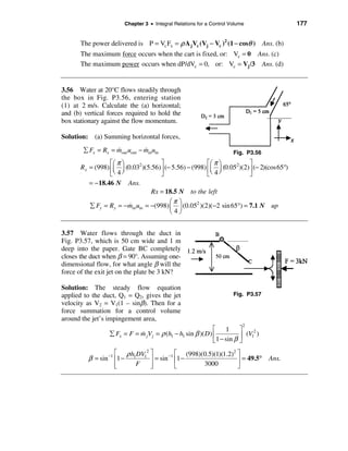

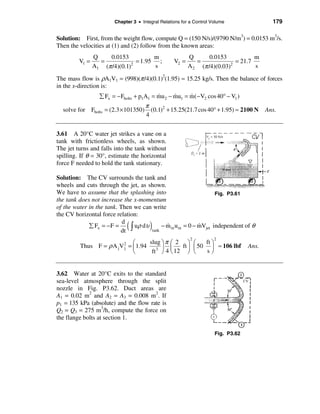
![180 Solutions Manual • Fluid Mechanics, Fifth Edition
Solution: With the known flow rates, we can compute the various velocities:
275/3600 m 3 /s m 550/3600 m
V2 = V3 = 2
= 9.55 ; V1 = = 7.64
0.008 m s 0.02 s
The CV encloses the split nozzle and cuts through the flange. The balance of forces is
å Fx = − Fbolts + p1,gage A1 = ρ Q 2 (− V2 cos 30°) + ρ Q 3 (−V3 cos30°) − ρ Q1 (+ V1 ),
æ 275 ö æ 550 ö
or: Fbolts = 2(998) ç ÷ (9.55cos30°) + 998 ç ÷ (7.64) + (135000 − 101350)(0.02)
è 3600 ø è 3600 ø
= 1261 + 1165 + 673 ≈ 3100 N Ans.
3.63 The sluice gate in Fig. P3.63 can
control and measure flow in open channels.
At sections 1 and 2, the flow is uniform and
the pressure is hydrostatic. The channel
width is b into the paper. Neglecting bottom
friction, derive an expression for the force F
required to hold the gate. For what condition
h2/h1 is the force largest? For very low
velocity V1 = gh1, for what value of h2/h1
2 Fig. P3.63
will the force be one-half of the maximum?
Solution: The CV encloses the inlet and exit and the whole gate, as shown. From mass
conservation, the velocities are related by
V1h1b = V2 h 2 b, or: V2 = V1 (h1 /h 2 )
The bottom pressures at sections 1&2 equal ρgh1 and ρgh2, respectively. The horizontal
force balance is
1 1
å Fx = − Fgate +ρ gh1 (h1b) − ρ gh2 (h2 b) = m(V2 − V1 ), m = ρ h1bV1
& &
2 2
1 2 éh ù
Solve for Fgate = ρ gbh1 [1 − (h 2 /h1 )2 ] − ρ h1bV1 ê 1 − 1ú Ans.
2
2 ë h2 û
For everything held constant except h2, the maximum force occurs when
1/3
h 2 æ V1 ö
( )
2
dF 1/3
= 0 which yields h 2 = V12 h1 /g
2
or: ≈ç ÷ Ans.
dh 2 h1 è gh1 ø
(
Finally, for very low velocity, only the first term holds: F ≈ (1/2)ρ gb h1 − h 2 . In this
2
2 )
case the maximum force occurs when h2 = 0, or Fmax = (1/2)ρgbh1 . (Clearly this is the
2](https://image.slidesharecdn.com/solucionariodefluidoswhite-120604143132-phpapp02/85/Solucionario-de-fluidos_white-180-320.jpg)

![182 Solutions Manual • Fluid Mechanics, Fifth Edition
3.66 The tank in Fig. P3.66 weighs 500 N
empty and contains 600 L of water at 20°C.
Pipes 1 and 2 have D = 6 cm and Q =
300 m3/hr. What should the scale reading
W be, in newtons?
Solution: Let the CV surround the tank,
cut through the two jets, and slip just under Fig. P3.66
the tank bottom, as shown. The relevant jet
velocities are
Q (300/3600) m 3 /s
V1 = V2 = = ≈ 29.5 m/s
A (π /4)(0.06 m)2
The scale reads force “P” on the tank bottom. Then the vertical force balance is
å Fz = P − Wtank − Wwater = m2 v2 − m1v1 = m[0 − (−V1 )]
& & &
æ 300 ö
Solve for P = 500 + 9790(0.6 m 3 ) + 998 ç ÷ (29.5) ≈ 8800 N Ans.
è 3600 ø
3.67 Gravel is dumped from a hopper, at a rate of 650 N/s, onto a moving belt, as in
Fig. P3.67. The gravel then passes off the end of the belt. The drive wheels are 80 cm in
diameter and rotate clockwise at 150 r/min. Neglecting system friction and air drag,
estimate the power required to drive this belt.
Fig. P3.67
Solution: The CV goes under the gravel on the belt and cuts through the inlet and
outlet gravel streams, as shown. The no-slip belt velocity must be
é rev rad 1 min ù m
Vbelt = Voutlet = ΩR wheel = ê150 2π ú (0.4 m) ≈ 6.28 s
ë min rev 60 s û](https://image.slidesharecdn.com/solucionariodefluidoswhite-120604143132-phpapp02/85/Solucionario-de-fluidos_white-182-320.jpg)


![186 Solutions Manual • Fluid Mechanics, Fifth Edition
Solution: First convert 300 gal/min = 0.01893 m3/s, hence the mass flow is ρQ = 18.9 kg/s.
The vertical-tube velocity (down) is Vtube = 0.01893/[(π/4)(0.06)2] = −6.69 k m/s. The
exit tube area is (π/2)R∆h = (π/2)(0.15)(0.01) = 0.002356 m2, hence Vexit = Q/Aexit =
0.01893/0.002356 = 8.03 m/s. Now estimate the force components:
+45°
å Fx = Fx = ò uout dmout =
& ò −Vexit sinθ ρ ∆hR dθ ≡ 0 Ans. (a)
−45°
+45°
å Fy = Fy = ò vout dmout − mvin =
& & ò −Vexit cosθ ρ ∆hR dθ − 0 = −Vexit ρ∆hR 2
−45°
or: Fy = −(8.03)(998)(0.01)(0.15) 2 ≈ −17 N Ans. (b)
å Fz = Fz = m(wout − win ) = (18.9 kg/s)[0 − (−6.69 m/s)] ≈ +126 N
& Ans. (c)
3.75 A liquid jet of density r and area A
strikes a block and splits into two jets, as
shown in the figure. All three jets have the
same velocity V. The upper jet exits at angle
θ and area αA, the lower jet turns down at
90° and area (1 − α)A. (a) Derive a formula
for the forces (Fx,Fy) required to support
the block against momentum changes.
(b) Show that Fy = 0 only if α ≥ 0.5.
(c) Find the values of α and θ for which both
Fx and Fy are zero.
Solution: (a) Set up the x- and y-momentum relations:
å Fx = Fx = α m(−V cosθ ) − m(−V ) where m = ρ AV of the inlet jet
& & &
å Fy = Fy = α mV sinθ + (1 − α )m(−V )
& &
Clean this up for the final result:
Fx = mV(1 − α cosθ )
&
Fy = mV(α sin θ + α − 1) Ans. (a)
&
(b) Examining Fy above, we see that it can be zero only when,
1−α
sinθ =
α
But this makes no sense if α < 0.5, hence Fy = 0 only if α ≥ 0.5. Ans. (b)](https://image.slidesharecdn.com/solucionariodefluidoswhite-120604143132-phpapp02/85/Solucionario-de-fluidos_white-186-320.jpg)
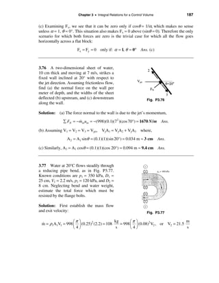
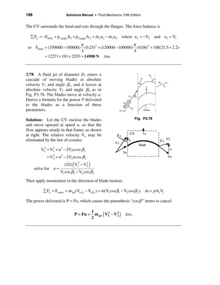

![192 Solutions Manual • Fluid Mechanics, Fifth Edition
The air density is ρ = p/RT = (101350)/[287(293)] ≈ 1.205 kg/m3. We are not given any
pressures on the cone so we consider momentum only. The force balance is
å Fx = Fcone = m(uout − u in ) = (1.205)(0.736)(57.6 cos 45° − 15) ≈ 22.8 N
& Ans.
The force on the cone is to the right because we neglected pressure forces.
3.85 The thin-plate orifice in Fig. P3.85
causes a large pressure drop. For 20°C water
flow at 500 gal/min, with pipe D = 10 cm
and orifice d = 6 cm, p1 − p2 ≈ 145 kPa. If
the wall friction is negligible, estimate the
force of the water on the orifice plate.
Fig. P3.85
Solution: The CV is inside the pipe walls, cutting through the orifice plate, as shown.
At least to one-dimensional approximation, V1 = V2, so there is no momentum change.
The force balance yields the force of the plate on the fluid:
å Fx = − Fplate on fluid + p1A1 − p2 A 2 − τ wall A wall = m(V2 − V1 ) ≈ 0
&
π
Since τ wall ≈ 0, we obtain Fplate = (145000) (0.1)2 ≈ 1140 N Ans.
4
The force of the fluid on the plate is opposite to the sketch, or to the right.
3.86 For the water-jet pump of Prob. 3.36,
add the following data: p1 = p2 = 25 lbf/in2,
and the distance between sections 1 and 3
is 80 in. If the average wall shear stress
between sections 1 and 3 is 7 lbf/ft2, esti-
mate the pressure p3. Why is it higher than p1?
Fig. P3.36
Solution: The CV cuts through sections 1, 2, 3 and along the inside pipe walls. Recall
from Prob. 3.36 that mass conservation led to the calculation V3 ≈ 6.33 m/s. Convert data
to SI units: L = 80 in = 2.032 m, p1 = p2 = 25 psi = 172.4 kPa, and τwall = 7 psf = 335 Pa.
We need mass flows for each of the three sections:
æπ ö kg
m1 = 998 ç ÷ (0.0762)2 (40) ≈ 182
& ;
è4ø s
æπ ö kg kg
m 2 = 998 ç ÷ [(0.254)2 − (0.0762)2 ](3) ≈ 138
& and m 3 ≈ 182 + 138 ≈ 320
&
è4ø s s](https://image.slidesharecdn.com/solucionariodefluidoswhite-120604143132-phpapp02/85/Solucionario-de-fluidos_white-192-320.jpg)
![194 Solutions Manual • Fluid Mechanics, Fifth Edition
Solution: Let the CV move to the left at boat speed V and enclose the boat and the
pump’s inlet and exit. Then the momentum relation is
å Fx = kV 2 = m pump (Vj + V − Vinlet ) ≈ ρ Q(Vj + V) if we assume Vinlet = Vj
&
If, further, V = Vj , then the approximate solution is: V ≈ (ρ QVj/k)1/2 Ans.
If V and Vj are comparable, then we solve a quadratic equation:
ρQ
V ≈ ζ + [ζ 2 + 2ζ Vj ]1/2, where ζ = Ans.
2k
3.89 Consider Fig. P3.36 as a general problem for analysis of a mixing ejector pump. If
all conditions (p, ρ, V) are known at sections 1 and 2 and if the wall friction is negligible,
derive formulas for estimating (a) V3 and (b) p3.
Solution: Use the CV in Prob. 3.86 but use symbols throughout. For volume flow,
π 2 π 2 π 2
4 4
( 4
)
V1 D1 + V2 D2 − D1 = V3 D2, or: V3 = V1α + V2 (1 − α ), α = (D1 /D2 )2
2
(A)
Now apply x-momentum, assuming (quite reasonably) that p1 = p2:
π 2 π 2 2 π 2 π 2 2
(p1 − p3 )
4
D2 − τ wπ D2 L = ρ D2 V3 − ρ
4 4
1( 2
4
)
D2 − D2 V 2 − ρ D1 V1
2
4Lτ w æD ö
Clean up: p3 = p1 − + ρ éα V1 + (1 − α )V2 − V 2 ù where α = ç 1 ÷
ë
2 2
3û Ans.
D2 è D2 ø
You have to insert V3 into this answer from Eq. (A) above, but the algebra is messy.
3.90 As shown in Fig. P3.90, a liquid
column of height h is confined in a vertical
tube of cross-sectional area A by a stopper.
At t = 0 the stopper is suddenly removed,
exposing the bottom of the liquid to
atmospheric pressure. Using a control-
volume analysis of mass and vertical
momentum, derive the differential equation
for the downward motion V(t) of the liquid.
Assume one-dimensional, incompressible,
frictionless flow. Fig. P3.90](https://image.slidesharecdn.com/solucionariodefluidoswhite-120604143132-phpapp02/85/Solucionario-de-fluidos_white-194-320.jpg)
![196 Solutions Manual • Fluid Mechanics, Fifth Edition
From mass conservation, V1 = V2 = V(t). For CV’s #1 and #2,
dV
å Fdown − ò a rel dm = ∆(mv) = 0 = (patm − p I )A + ρ gAh − m1
& (No. 1)
dt
dV
å Fx − ò a rel dm = ∆(mu) = 0 = (p I − patm )A + 0 − m 2
& (No. 2)
dt
Add these two together. The pressure terms cancel, and we insert the two blob masses:
dV dV h
ρ gAh − ( ρ Ah + ρ AL) = 0, or: =g Ans.
dt dt L+h
3.93 Extend Prob. 3.92 to include a linear (laminar) average wall shear stress of the form
τ ≈ cV, where c is a constant. Find V(t), assuming that the wall area remains constant.
Solution: For the same two CV’s as in Prob. 3.92 above, we add wall shears:
dV
∆pA + ρ gAh − (cV)π Dh = m1 (No. 1)
dt
dV
−∆pA + 0 − (cV)π DL = m 2 (No. 2)
dt
Add together, divide by (ρA), A = πD2/4, and rearrange into a 1st order linear ODE:
dV æ 4c ö gh
+ç ÷V = subject to V = 0 at t = 0, h = h o Ans.
dt è ρ D ø L+h
The blob length (L + h) could be assumed constant, but h = h(t). We could substitute for
V = −dh/dt and rewrite this relation as a 2nd order ODE for h(t), but we will not proceed
any further with an analytical solution to this differential equation.
3.94 Attempt a numerical solution of Prob. 3.93 for SAE 30 oil at 20°C. Let h = 20 cm,
L = 15 cm, and D = 4 mm. Use the laminar shear approximation from Sec. 6.4: τ ≈
8µV/D, where µ is the fluid viscosity. Account for the decrease in wall area wetted by the
fluid. Solve for the time required to empty (a) the vertical leg and (b) the horizontal leg.
Solution: For SAE 30 oil, µ ≈ 0.29 kg/(m · s) and ρ ≈ 917 kg/m3. For laminar flow as
given, c = 8µ/D, so the coefficient (4c/ρD) = 4[8(0.29)/0.004]/[917(0.004)] ≈ 632 s−1.
[The flow is highly damped.] Then the basic differential equation becomes
t
dV 9.81h
+ 632V = , with h = 0.2 − ò V dt and V(0) = 0
dt 0.15 + h 0](https://image.slidesharecdn.com/solucionariodefluidoswhite-120604143132-phpapp02/85/Solucionario-de-fluidos_white-196-320.jpg)

![200 Solutions Manual • Fluid Mechanics, Fifth Edition
3.99 Let the rocket of Fig. E3.12 start at z = 0, with constant exit velocity and exit mass
flow, and rise vertically with zero drag. (a) Show that, as long as fuel burning continues,
the vertical height S(t) reached is given by
Ve Mo &
mt
S= [ζ ln ζ − ζ + 1], where ζ = 1 −
m& Mo
(b) Apply this to the case Ve = 1500 m/s and Mo = 1000 kg to find the height reached after
a burn of 30 seconds, when the final rocket mass is 400 kg.
Solution: (a) Ignoring gravity effects, integrate the equation of the projectile’s velocity
(from E3.12):
t
é æ mt ö ù
&
S (t ) = ò V (t ) dt = ò ê −Ve ln ç 1 − ÷ ú dt
0 ë è Mo øû
&
mt m&
Let ζ = 1 − , then dζ = − dt and the integral becomes,
Mo Mo
ζ
é − Mo ù æV M ö ζ æV M ö
S(t ) = (−Ve ) ê
& ú
ë m û1
ò (ζ ln ζ ) dζ = ç em o ÷ [ζ ln ζ − ζ ]1 = ç em o ÷ [ζ ln ζ − ζ + 1]
è & ø è & ø
(b) Substituting the numerical values given,
∆M M f − M o 1000 kg − 400 kg (20 kg/s)(30 s)
m=
& = = = 20 kg/s and ζ = 1 − = 0.40
∆t ∆t 30 s 1000 kg
(1500 m/s)(1000 kg)
S (t = 30 s) = [0.4 ln(0.4) − (0.4) + 1] = 17, 500 m Ans.
(20 kg/s)
3.100 Suppose that the solid-propellant rocket of Prob. 3.35 is built into a missile of
diameter 70 cm and length 4 m. The system weighs 1800 N, which includes 700 N of
propellant. Neglect air drag. If the missile is fired vertically from rest at sea level, estimate
(a) its velocity and height at fuel burnout and (b) the maximum height it will attain.
Solution: The theory of Example 3.12 holds until burnout. Now Mo = 1800/9.81 =
183.5 kg, and recall from Prob. 3.35 that Ve = 1150 m/s and the exit mass flow is 11.8 kg/s.
The fuel mass is 700/9.81 = 71.4 kg, so burnout will occur at tburnout = 71.4/11.8 = 6.05 s.
Then Example 3.12 predicts the velocity at burnout:
æ 11.8(6.05) ö m
Vb = −1150 ln ç 1 − ÷ − 9.81(6.05) ≈ 507 Ans. (a)
è 183.5 ø s](https://image.slidesharecdn.com/solucionariodefluidoswhite-120604143132-phpapp02/85/Solucionario-de-fluidos_white-200-320.jpg)
![Chapter 3 • Integral Relations for a Control Volume 201
Meanwhile, Prob. 3.99 gives the formula for altitude reached at burnout:
183.5(1150) 1
Sb = [1 + (0.611){ln(0.611) − 1}] − (9.81)(0.605)2 ≈ 1393 m Ans. (a)
11.8 2
where “0.611” = 1 – 11.8(6.05)/183.5, that is, the mass ratio at burnout. After burnout,
with drag neglected, the missile moves as a falling body. Maximum height occurs at
Vo 507
∆t = = = 51.7 s, whence
g 9.81
1
S = So + g∆t 2 = 1393 + (1/2)(9.81)(51.7)2 ≈ 14500 m Ans. (b)
2
3.101 Modify Prob. 3.100 by accounting for air drag on the missile F ≈ CρD2V 2, where
C ≈ 0.02, ρ is the air density, D is the missile diameter, and V is the missile velocity.
Solve numerically for (a) the velocity and altitude at burnout and (b) the maximum
altitude attained.
Solution: The CV vertical-momentum analysis of Prob. 3.100 is modified to include a
drag force resisting the upward acceleration:
4.26
dV æ T − Bz ö
m = mVe − mg − CD ρ D2 V 2, where m = m o − mt, and
& & ρ = ρo ç o ÷
dt è To ø
kg m
with numerical values m o = 183.5 kg, m = 11.8
& , Ve = 1150 , D = 0.7 m, C D = 0.02
s s
We may integrate this numerically, by Runge-Kutta or a spreadsheet or whatever, starting
with V = 0, z = 0, at t = 0. After burnout, t ≈ 6.05 s, we drop the thrust term. The density
is computed for the U.S. Standard Atmosphere from Table A-6. The writer’s numerical
solution is shown graphically on the next page. The particular values asked for in the
problem are as follows:
At burnout, t = 6.05 s: V ≈ 470 m/s, z ≈ 1370 m Ans. (a)
At maximum altitude: t ≈ 40 s, z max ≈ 8000 m Ans. (b)
We see that drag has a small effect during rocket thrust but a large effect afterwards.](https://image.slidesharecdn.com/solucionariodefluidoswhite-120604143132-phpapp02/85/Solucionario-de-fluidos_white-201-320.jpg)
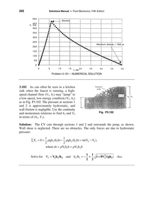
![Chapter 3 • Integral Relations for a Control Volume 203
3.103 Suppose that the solid-propellant rocket of Prob. 3.35 is mounted on a 1000-kg
car to propel it up a long slope of 15°. The rocket motor weighs 900 N, which includes
500 N of propellant. If the car starts from rest when the rocket is fired, and if air drag
and wheel friction are neglected, estimate the maximum distance that the car will travel
up the hill.
Solution: This is a variation of Prob. 3.100, except that “g” is now replaced by “g sinθ.”
Recall from Prob. 3.35 that the rocket mass flow is 11.8 kg/s and its exit velocity is 1150 m/s.
The rocket fires for tb = (500/9.81)/11.8 = 4.32 sec, and the initial mass is Mo = (1000 +
900/9.81) = 1092 kg. Then the differential equation for uphill powered motion is
dV
m = mVe − mg sinθ , m = M o − mt
& &
dt
This integrates to: V(t) = −Ve ln(1 − mt/Mo ) − gt sin θ
& for t ≤ 4.32 s.
After burnout, the rocket coasts uphill with the usual falling-body formulas with “g sinθ.”
The distance travelled during rocket power is modified from Prob. 3.99:
1
S = (Mo Ve /m)[1 + (1 − mt/M o ){ln(1 − mt/Mo ) − 1}] − gt 2 sin θ
& & &
2
Apply these to the given data at burnout to obtain
1
Vburnout = −1150 ln(0.9533) − (9.81)sin15°(4.32) ≈ 44.0 m/s
2
1092(1150) 1
Sburnout = [1 + 0.9533{ln(0.9533) − 1}] − (9.81)sin15°(4.32)2 ≈ 94 m
11.8 2
The rocket then coasts uphill a distance ∆S such that Vb2 = 2g∆S sinθ, or ∆S =
(44.0)2/[2(9.81)sin 15°] ≈ 381 m. The total distance travelled is 381 + 94 ≈ 475 m Ans.
3.104 A rocket is attached to a rigid
horizontal rod hinged at the origin as in
Fig. P3.104. Its initial mass is Mo, and its
&
exit properties are m and Ve relative to the
rocket. Set up the differential equation for
rocket motion, and solve for the angular
velocity ω (t) of the rod. Neglect gravity, air
drag, and the rod mass. Fig. P3.104](https://image.slidesharecdn.com/solucionariodefluidoswhite-120604143132-phpapp02/85/Solucionario-de-fluidos_white-203-320.jpg)
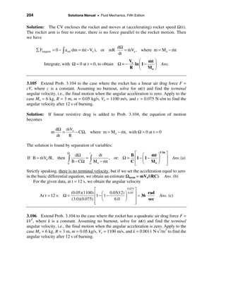
 ≈ 2900 N
& Ans.
3.108 A rocket sled of mass M is to be
decelerated by a scoop, as in Fig. P3.108,
which has width b into the paper and dips into
the water a depth h, creating an upward jet at
60°. The rocket thrust is T to the left. Let the
initial velocity be Vo, and neglect air drag and
wheel friction. Find an expression for V(t) of
the sled for (a) T = 0 and (b) finite T ≠ 0. Fig. P3.108](https://image.slidesharecdn.com/solucionariodefluidoswhite-120604143132-phpapp02/85/Solucionario-de-fluidos_white-205-320.jpg)
![206 Solutions Manual • Fluid Mechanics, Fifth Edition
Solution: The CV surrounds the sled and scoop and moves to the left at sled speed V(t).
Let x be positive to the left. The horizontal force balance is
dV
å Fx = T − M = m out u out − m in u in = m( −V cosθ ) − m( −V), m = ρ bhV
& & & & &
dt
dV
or: Msled = T − CV 2, C = ρ bh(1 − cosθ )
dt
Whether or not thrust T = 0, the variables can be separated and integrated:
V t
dV C Vo
(a) T = 0: ò V 2
= − ò dt, or: V =
M0 1 + CVo t/M
Ans. (a)
Vo
V t
M dV
(b) T > 0: ò T − CV 2 ò
= dt, or: V = Vfinal tanh[α t + φ ] Ans. (b)
Vo 0
where Vfinal = [T/ρ bg(1 − cosθ )]1/2, α = [Tρ bh(1 − cosθ )]1/2 /M, φ = tanh −1 (Vo /Vf )
This solution only applies when Vo < Vfinal, which may not be the case for a speedy sled.
3.109 Apply Prob. 3.108 to the following data: Mo = 900 kg, b = 60 cm, h = 2 cm, Vo =
120 m/s, with the rocket of Prob. 3.35 attached and burning. Estimate V after 3 sec.
Solution: Recall from Prob. 3.35 that the rocket had a thrust of 13600 N and an exit
mass flow of 11.8 kg/s. Then, after 3 s, the mass has only dropped to 900 – 11.8(3) = 865 kg,
so we can approximate that, over 3 seconds, the sled mass is near constant at about 882 kg.
Compute the “final” velocity if the rocket keeps burning:
1/2
é 13600 ù m
Vfinal = [T/{ρ bh(1 − cosθ )}] 1/2
=ê ú ≈ 47.66
ë 998(0.6)(0.02)(1 − cos 60°) û s
Thus solution (b) to Prob. 3.108 does not apply, since Vo = 120 m/s > Vfinal. We therefore
effect a numerical solution of the basic differential equation from Prob. 3.108:
dV dV m
M = T − ρ bh(1 − cosθ )V 2 , or: 882 = 13600 − 5.988V 2, with Vo = 120
dt dt s
The writer solved this on a spreadsheet for 0 < t < 3 sec. The results may be tabulated:
t, sec: 0.0 0.5 1.0 1.5 2.0 2.5 3.0 sec
V, m/s: 120.0 90.9 75.5 66.3 60.4 56.6 53.9 m/s
The sled has decelerated to 53.9 m/s, quite near its “steady” speed of about 46 m/s.](https://image.slidesharecdn.com/solucionariodefluidoswhite-120604143132-phpapp02/85/Solucionario-de-fluidos_white-206-320.jpg)
![Chapter 3 • Integral Relations for a Control Volume 207
3.110 The horizontal lawn sprinkler in
Fig. P3.110 has a water flow rate of
4.0 gal/min introduced vertically through
the center. Estimate (a) the retarding torque
required to keep the arms from rotating and Fig. P3.110
(b) the rotation rate (r/min) if there is no re-
tarding torque.
Solution: The flow rate is 4 gal/min = 0.008912 ft3/s, and ρ = 1.94 slug/ft3. The
velocity issuing from each arm is Vo = (0.008912/2)/[(π/4)(0.25/12 ft)2] ≈ 13.1 ft/s. Then:
Vo To
(a) From Example 3.15, ω = − and, if there is no motion (ω = 0),
R ρ QR 2
To = ρ QRVo = (1.94)(0.008912)(6/12)(13.1) ≈ 0.113 ft-lbf Ans. (a)
13.1 ft/s rad rev
(b) If To = 0, then ω no friction = Vo /R = = 26.14 ≈ 250 Ans. (b)
6/12 ft s min
3.111 In Prob. 3.60 find the torque caused
around flange 1 if the center point of exit 2
is 1.2 m directly below the flange center.
Solution: The CV encloses the elbow
and cuts through flange (1). Recall from
Prob. 3.60 that D1 = 10 cm, D2 = 3 cm,
weight flow = 150 N/s, whence V1 = 1.95 m/s
and V2 = 21.7 m/s. Let “O” be in the center Fig. P3.60
of flange (1). Then rO2 = −1.2j and rO1 = 0.
The pressure at (1) passes through O, thus causes no torque. The moment relation is
& æ 150 kg ö
å M O = TO = m[(rO2 × V2 ) − (rO1 × V1 )] = ç ÷ [(−1.2 j) × (−16.6 i − 13.9 j)]
è 9.81 s ø
or: TO = −305 k N ⋅ m Ans.
3.112 The wye joint in Fig. P3.112 splits
the pipe flow into equal amounts Q/2,
which exit, as shown, a distance Ro from
the axis. Neglect gravity and friction. Find
an expression for the torque T about the
x axis required to keep the system rotating
at angular velocity Ω.
Fig. P3.112](https://image.slidesharecdn.com/solucionariodefluidoswhite-120604143132-phpapp02/85/Solucionario-de-fluidos_white-207-320.jpg)

![Chapter 3 • Integral Relations for a Control Volume 209
3.114 The 3-arm lawn sprinkler of
Fig. P3.114 receives 20°C water through
the center at 2.7 m3/hr. If collar friction is
neglected, what is the steady rotation rate
in rev/min for (a) θ = 0°; (b) θ = 40°?
Solution: The velocity exiting each arm is
Q/3 2.7/[(3600)(3)] m
Vo = = = 6.50
(π /4)d 2
(π /4)(0.007) 2
s Fig. P3.114
With negligible air drag and bearing friction,
the steady rotation rate (Example 3.15) is
Vo cosθ (6.50) cos 0° rad rev
ω final = (a) θ = 0°: ω = = 43.3 = 414 Ans. (a)
R 0.15 m s min
rev
(b) θ = 40° : ω = ω o cosθ = (414) cos 40° = 317 Ans. (b)
min
3.115 Water at 20°C flows at 30 gal/min
through the 0.75-in-diameter double pipe
bend of Fig. P3.115. The pressures are p1 =
30 lbf/in2 and p2 = 24 lbf/in2. Compute the
torque T at point B necessary to keep the
pipe from rotating.
Solution: This is similar to Example 3.13,
of the text. The volume flow Q = 30 gal/min = Fig. P3.115
0.0668 ft3/s, and ρ = 1.94 slug/ft3. Thus the
mass flow ρQ = 0.130 slug/s. The velocity
in the pipe is
0.0668 ft
V1 = V2 = Q/A = = 21.8
(π /4)(0.75/12) 2
s
If we take torques about point B, then the distance “h1,” from p. 143, = 0, and h2 = 3 ft.
The final torque at point B, from “Ans. (a)” on p. 143 of the text, is
π
TB = h 2(p 2 A 2 + mV2 ) = (3 ft)[(24 psi) (0.75 in)2 + (0.130)(21.8)] ≈ 40 ft ⋅ lbf
& Ans.
4](https://image.slidesharecdn.com/solucionariodefluidoswhite-120604143132-phpapp02/85/Solucionario-de-fluidos_white-209-320.jpg)
![212 Solutions Manual • Fluid Mechanics, Fifth Edition
3.119 Revisit the turbine cascade system
of Prob. 3.78, and derive a formula for the
power P delivered, using the angular-
momentum theorem of Eq. (3.55).
Solution: To use the angular momentum
theorem, we need the inlet and outlet
velocity diagrams, as in the figure. The
Euler turbine formula becomes
To = ρ Q(r1Vt1 − r2 Vt2 ) ≈ ρ QR(Vt1 − Vt2 )
since the blades are at nearly constant radius R. From the velocity diagrams, we find
Vt1 = u + Vn1 cot α1; Vt2 = u − Vn2 cot α 2 , where Vn1 = Vn2 = V1 cos β1
The normal velocities are equal by virtue of mass conservation across the blades. Finally,
P = ρ Qω R(Vt1 − Vt2 ) = ρ QuVn (cotα 1 + cotα 2 ) Ans.
3.120 A centrifugal pump delivers 4000 gal/min of water at 20°C with a shaft rotating
at 1750 rpm. Neglect losses. If r1 = 6 in, r2 = 14 in, b1 = b2 = 1.75 in, Vt1 = 10 ft/s, and Vt2 =
110 ft/s, compute the absolute velocities (a) V1 and (b) V2, and (c) the ideal horsepower
required.
Solution: First convert 4000 gal/min = 8.91 ft3/s and 1750 rpm = 183 rad/s. For water,
take ρ = 1.94 slug/ft3. The normal velocities are determined from mass conservation:
Q 8.91 ft Q ft
Vn1 = = = 19.5 ; Vn2 = = 8.34
2π r1b1 2π (6/12)(1.75/12) s 2π r2 b2 s
Then the desired absolute velocities are simply the resultants of Vt and Vn:
ft ft
V1 = [(10)2 + (19.45)2 ]1/2 = 22 V2 = [(110)2 + (8.3)2 ]1/2 = 110 Ans. (a, b)
s s
The ideal power required is given by Euler’s formula:
P = ρ Qω (r2 Vt2 − r1Vt1 ) = (1.94)(8.91)(183)[(14/12)(110) − (6/12)(10)]
ft-lbf
= 391,000 ≈ 710 hp Ans. (c)
s](https://image.slidesharecdn.com/solucionariodefluidoswhite-120604143132-phpapp02/85/Solucionario-de-fluidos_white-212-320.jpg)
![Chapter 3 • Integral Relations for a Control Volume 213
3.121 The pipe bend of Fig. P3.121 has
D1 = 27 cm and D2 = 13 cm. When water at
20°C flows through the pipe at 4000 gal/
min, p1 = 194 kPa (gage). Compute the
torque required at point B to hold the bend
stationary.
Solution: First convert Q = 4000 gal/
min = 0.252 m3/s. We need the exit velocity: Fig. P3.121
0.252 m m
V2 = Q/A 2 = = 19.0 Meanwhile, V1 = Q/A1 = 4.4
(π /4)(0.13) 2
s s
We don’t really need V1, because it passes through B and has no angular momentum. The
angular momentum theorem is then applied to point B:
&
å M B = TB + r1 × p1A1 j + r2 × p2 A 2 (− i) = m(r2 × V2 − r1 × V1 )
But r1 and p2 are zero,
hence TB = m(r2 × V2 ) = ρ Q[(0.5i + 0.5 j) × (19.0i)]
&
Thus, finally, TB = (998)(0.252)(0.5)(19.0)(−k) ≈ −2400 k N · m (clockwise) Ans.
3.122 Extend Prob. 3.46 to the problem
of computing the center of pressure L of
the normal face Fn, as in Fig. P3.122. (At
the center of pressure, no moments are
required to hold the plate at rest.) Neglect
friction. Express your result in terms of the
sheet thickness h1 and the angle θ between
the plate and the oncoming jet 1.
Fig. P3.122
Solution: Recall that in Prob. 3.46 of this Manual, we found h2 = (h1/2)(1 + cosθ) and
that h3 = (h1/2)(1 − cosθ). The force on the plate was Fn = ρQVsinθ. Take clockwise
moments about O and use the angular momentum theorem:
å Mo = − Fn L = m 2 |r2O × V2 | z + m 3 |r3O × V3 | z − m1|r1O × V1 | z
& & &
(
= ρ Vh 2 (h 2 V/2) + ρ Vh3 (− h3 V/2) − 0 = (1/2) ρ V 2 h 2 − h 3
2
2
)](https://image.slidesharecdn.com/solucionariodefluidoswhite-120604143132-phpapp02/85/Solucionario-de-fluidos_white-213-320.jpg)

![Chapter 3 • Integral Relations for a Control Volume 215
Solution: First we need the mass flow and velocity from each hole “i,” i = 1 to 6:
Q i (3.0/448.8)/6 ft ρQ æ 3/448.8 ö slug
Vi = = 2
≈ 5.81 &
mi = = 1.94 ç ÷ = 0.00216
Ai æ 3/16 ö s 6 è 6 ø s
(π /4) ç ÷
è 12 ø
Recall Example 3.15 from the text. For each hole, we need the absolute velocity, Vi − Ωri.
The angular momentum theorem is then applied to moments about point O:
å M O = TO = å m i (riO × Vi, abs ) − m in Vin = å m i ri (Vi cos 40° − Ωri )
& & &
All the velocities and mass flows from each hole are equal. Then, if TO = 0 (no friction),
&
å m i ri Vi cos 40° å ri 5.33 rad
Ω= = Vi cos40° 2 = (5.81)(0.766) = 4.25 = 41 rpm Ans.
&
å miri 2
å ri 5.58 s
3.125 A liquid of density ρ flows through
a 90° bend as in Fig. P3.125 and issues
vertically from a uniformly porous section
of length L. Neglecting weight, find a
result for the support torque M required at
point O.
Solution: Mass conservation requires i
Fig. P3.125
L
dQ
Q = ò Vw (π d) dx = Vwπ dL, or: = π dVw
0
dx
Then the angular momentum theorem applied to moments about point O yields
L
å M O = TO = ò (rO × V )dm out = k ò (R + x)Vw ρπ dVw dx
&
CS 0
ρπ dVw [(R + x)2 − R 2 ] |0
k L
= 2
2
æ Lö
Substitute Vwπ dL = Q and clean up to obtain TO = ρ QVwç R + ÷ k Ans.
è 2ø](https://image.slidesharecdn.com/solucionariodefluidoswhite-120604143132-phpapp02/85/Solucionario-de-fluidos_white-215-320.jpg)

![Chapter 3 • Integral Relations for a Control Volume 217
Solution: For water, take cp ≈ 4280 J/kg · °C. For an overall CV enclosing the entire
sketch,
& & &
Q = m out (c p Tout ) − m in (c p Tin ),
or: 55, 000, 000 W ≈ (998 × 2.5)[4280Tout − 4280(18)], solve for Tout ≈ 23.15°C Ans.
The power plant flow is “internal” to the CV, hence Q out = Q in = 2.5 m 3 /s. Ans.
3.128 For the conditions of Prob. 3.127, if the power plant is to heat the nearby river
water by no more than 12°C, what should be the minimum flow rate Q, in m3/s, through
the plant heat exchanger? How will the value of Q affect the downstream conditions
(Qo, To)?
Solution: Now let the CV only enclose the power plant, so that the flow going through
the plant shows as an inlet and an outlet. The CV energy equation, with no work, gives
& & &
Q plant = m out c p Tout − m in c p Tin = (998)Q plant (4280)(12°C) since Q in = Q out
55,000,000
Solve for Q plant = ≈ 1.07 m 3 /s Ans.
(998)(4280)(12)
It’s a lot of flow, but if the river water mixes well, the downstream flow is still the same.
3.129 Multnomah Falls in the Columbia River Gorge has a sheer drop of 543 ft. Use the
steady flow energy equation to estimate the water temperature rise, in °F, resulting.
Solution: For water, convert cp = 4200 × 5.9798 = 25100 ft·lbf/(slug·°F). Use the
steady flow energy equation in the form of Eq. (3.66), with “1” upstream at the top of
the falls:
1 2 1
ᐈ1 + V1 + gz1 = ᐈ2 + V 2 + gz 2 − q
2
2 2
Assume adiabatic flow, q = 0 (although evaporation might be important), and neglect the
kinetic energies, which are much smaller than the potential energy change. Solve for
32.2(543)
∆ᐈ = c p ∆T ≈ g(z1 − z 2 ), or: ∆T = ≈ 0.70° F Ans.
25100](https://image.slidesharecdn.com/solucionariodefluidoswhite-120604143132-phpapp02/85/Solucionario-de-fluidos_white-217-320.jpg)
![218 Solutions Manual • Fluid Mechanics, Fifth Edition
3.130 When the pump in Fig. P3.130
draws 220 m3/h of water at 20°C from the
reservoir, the total friction head loss is 5 m.
The flow discharges through a nozzle to
the atmosphere Estimate the pump power
in kW delivered to the water.
Solution: Let “1” be at the reservoir surface
and “2” be at the nozzle exit, as shown. We
need to know the exit velocity:
Fig. P3.130
220/3600 m
V2 = Q/A 2 = = 31.12 , while V1 ≈ 0 (reservoir surface)
π (0.025) 2
s
Now apply the steady flow energy equation from (1) to (2):
2
p1 V1 p V2
+ + z1 = 2 + 2 + z 2 + h f − h p ,
ρ g 2g ρ g 2g
or: 0 + 0 + 0 = 0 + (31.12)2 /[2(9.81)] + 2 + 5 − h p, solve for h p ≈ 56.4 m.
The pump power P = ρgQhp = (998)(9.81)(220/3600)(56.4)
= 33700 W = 33.7 kW Ans.
3.131 When the pump in Fig. P3.130 delivers 25 kW of power to the water, the friction
head loss is 4 m. Estimate (a) the exit velocity; and (b) the flow rate.
Solution: The energy equation just above must now be written with V2 and Q
unknown:
2
V2 P 25000
0+0+0 = 0+ + 2 + 4 − h p , where h p = =
2g ρ gQ (998)(9.81)Q
Q
and where V2 = . Solve numerically by iteration: V2 ≈ 28.1 m/s Ans. (a)
π (0.025)2
and Q = (28.1)π(0.025)2 ≈ 0.0552 m3/s ≈ 200 m3/hr Ans. (b)](https://image.slidesharecdn.com/solucionariodefluidoswhite-120604143132-phpapp02/85/Solucionario-de-fluidos_white-218-320.jpg)
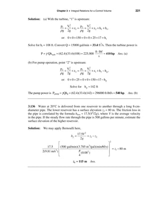
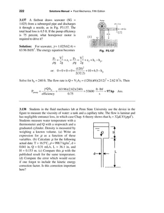
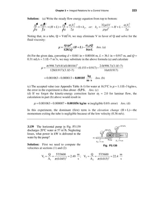

![Chapter 3 • Integral Relations for a Control Volume 225
Solution: First evaluate the average velocity in the pipe and the friction head loss:
1500 ft 3 Q 3.34 ft (17.0)2
Q= = 3.34 , so V = = = 17.0 and h f = 27 ≈ 121 ft
448.8 s A π (3/12) 2
s 2(32.2)
Then apply the steady flow energy equation:
2
p1 V1 p V2
+ + z1 = 2 + 2 + z 2 + h f − h p ,
ρ g 2g ρ g 2g
or: 0 + 0 + 50 = 0 + 0 + 150 + 121 − h p
γ Qh p (62.4)(3.34)(221)
Thus h p = 221 ft, so Ppump = =
η 0.75
ft ⋅ lbf
= 61600 ≈ 112 hp Ans.
s
3.142 A typical pump has a head which,
for a given shaft rotation rate, varies with
the flow rate, resulting in a pump
performance curve as in Fig. P3.142.
Suppose that this pump is 75 percent
efficient and is used for the system in
Prob. 3.141. Estimate (a) the flow rate, in
gal/min, and (b) the horsepower needed to
drive the pump.
Fig. P3.142
Solution: This time we do not know the flow rate, but the pump head is hp ≈ 300 −
50Q, with Q in cubic feet per second. The energy equation directly above becomes,
V2 π
0 + 0 + 50 = 0 + 0 + 150 + (27) − (300 − 50Q), where Q = V (0.5 ft)2
2(32.2) 4
This becomes the quadratic Q 2 + 4.60Q − 18.4 = 0, solve for Q ≈ 2.57 ft 3 /s
γ Qh p (62.4)(2.57)[300 − 50(2.57)]
Then the power is Ppump = =
η 0.75
ft ⋅ lbf
= 36700 ≈ 67 hp Ans.
s](https://image.slidesharecdn.com/solucionariodefluidoswhite-120604143132-phpapp02/85/Solucionario-de-fluidos_white-225-320.jpg)
![226 Solutions Manual • Fluid Mechanics, Fifth Edition
3.143 The insulated tank in Fig. P3.143 is
to be filled from a high-pressure air supply.
Initial conditions in the tank are T = 20°C
and p = 200 kPa. When the valve is opened,
the initial mass flow rate into the tank is
0.013 kg/s. Assuming an ideal gas, estimate Fig. P3.143
the initial rate of temperature rise of the air in
the tank.
Solution: For a CV surrounding the tank, with unsteady flow, the energy equation is
æ ö & &
d
dt
( ò e ρ dυ ) − m
in&çu+ +
ˆ
p V2
ρ 2
+ gz ÷ = Q − Wshaft = 0, neglect V 2 /2 and gz
è ø
d dT dρ
Rewrite as ( ρυ c v T) ≈ m in c p Tin = ρυ c v
& + c v Tυ
dt dt dt
where ρ and T are the instantaneous conditions inside the tank. The CV mass flow gives
dρ
d
dt
( ò ρ dυ ) − m
& in = 0, or: υ
dt
= m in
&
Combine these two to eliminate υ(dρ/dt) and use the given data for air:
dT m(c p − c v )T
& (0.013)(1005 − 718)(293) °C
= = ≈ 3.2 Ans.
ρυ c v
tank
dt é 200000 ù 3 s
ê 287(293) ú (0.2 m )(718)
ë û
3.144 The pump in Fig. P3.144 creates
a 20°C water jet oriented to travel a maxi-
mum horizontal distance. System friction
head losses are 6.5 m. The jet may be
approximated by the trajectory of friction-
less particles. What power must be deli-
Fig. P3.144
vered by the pump?
Solution: For maximum travel, the jet must exit at θ = 45°, and the exit velocity must be
[2(9.81)(25)]1/2 m
V2 sin θ = 2g ∆z max or: V2 = ≈ 31.32
sin 45° s
The steady flow energy equation for the piping system may then be evaluated:
p1 /γ + V1 /2g + z1 = p2 /γ + V 2 /2g + z 2 + h f − h p ,
2 2](https://image.slidesharecdn.com/solucionariodefluidoswhite-120604143132-phpapp02/85/Solucionario-de-fluidos_white-226-320.jpg)
![Chapter 3 • Integral Relations for a Control Volume 227
or: 0 + 0 + 15 = 0 + (31.32)2 /[2(9.81)] + 2 + 6.5 − h p , solve for h p ≈ 43.5 m
éπ ù
Then Ppump = γ Qh p = (9790) ê (0.05)2 (31.32)ú (43.5) ≈ 26200 W Ans.
ë4 û
3.145 The large turbine in Fig. P3.145
diverts the river flow under a dam as
shown. System friction losses are hf =
3.5V 2 /(2g), where V is the average velocity
in the supply pipe. For what river flow rate
in m3/s will the power extracted be 25 MW?
Which of the two possible solutions has a
better “conversion efficiency”?
Fig. P3.145
Solution: The flow rate is the unknown, with the turbine power known:
2
p1 V1 p V2
+ + z1 = 2 + 2 + z 2 + h f + h turb , or: 0 + 0 + 50 = 0 + 0 + 10 + h f + h turb
γ 2g γ 2g
Q
where h f = 3.5Vpipe /(2g) and h p = Pp /(γ Q) and Vpipe =
2
(π /4)D2 pipe
Introduce the given numerical data (e.g. Dpipe = 4 m, Ppump = 25E6 W) and solve:
Q3 − 35410Q + 2.261E6 = 0, with roots Q = +76.5, + 137.9, and − 214.4 m 3 /s
The negative Q is nonsense. The large Q (=137.9) gives large friction loss, hf ≈ 21.5 m.
The smaller Q (= 76.5) gives hf ≈ 6.6 m, about right. Select Qriver ≈ 76.5 m3/s. Ans.
3.146 Kerosene at 20°C flows through the
pump in Fig. P3.146 at 2.3 ft3/s. Head losses
between 1 and 2 are 8 ft, and the pump
delivers 8 hp to the flow. What should the
mercury-manometer reading h ft be?
Solution: First establish the two velocities:
Q 2.3 ft 3 /s
V1 = =
A1 (π /4)(3/12 ft)2 Fig. P3.146
ft 1 ft
= 46.9 ; V2 = V1 = 11.7
s 4 s](https://image.slidesharecdn.com/solucionariodefluidoswhite-120604143132-phpapp02/85/Solucionario-de-fluidos_white-227-320.jpg)

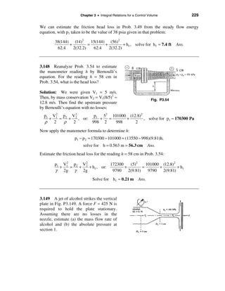
![230 Solutions Manual • Fluid Mechanics, Fifth Edition
Solution: A momentum analysis of the plate (e.g. Prob. 3.40) will give
π
F = mV2 = ρ A 2 V 2 = 0.79(998)
& 2
(0.02)2 V 2 = 425 N,
2
4
solve for V2 ≈ 41.4 m/s
whence m = 0.79(998)(π /4)(0.02)2 (41.4) ≈ 10.3 kg/s
& Ans. (a)
We find V1 from mass conservation and then find p1 from Bernoulli with no losses:
2
æ2ö
Incompressible mass conservation: V1 = V2 (D2 /D1 )2 = (41.4) ç ÷ ≈ 6.63 m/s
è5ø
Bernoulli, z1 = z 2 : p1 = p2 +
1
2
( 2 2
)
ρ V2 − V1 = 101000 +
0.79(998)
2
[(41.4)2 − (6.63)2 ]
≈ 760, 000 Pa Ans. (b)
3.150 An airfoil at an angle of attack
α, as in Fig. P3.150, provides lift by
a Bernoulli effect, because the lower
surface slows the flow (high pressure)
and the upper surface speeds up the flow
(low pressure). If the foil is 1.5 m long
and 18 m wide into the paper, and the
ambient air is 5000 m standard atmo-
sphere, estimate the total lift if the average Fig. P3.150
velocities on upper and lower surfaces are
215 m/s and 185 m/s, respectively. Neglect
gravity.
Solution: A vertical force balance gives,
FLift = ( pl − pu ) Aplanform =
1
2
( )
ρ Vu2 − Vl2 (bL )
1
= (0.7361)(2152 − 1852 )(18)(1.5)
2
= 119, 250 N = 119 kN Ans.](https://image.slidesharecdn.com/solucionariodefluidoswhite-120604143132-phpapp02/85/Solucionario-de-fluidos_white-230-320.jpg)

![Chapter 3 • Integral Relations for a Control Volume 233
Maximum X occurs at h = H/2, or Xmax = H. When h = 0.25H or 0.75H, the jet travels
out to H = 0.866H. These three trajectories are shown in the sketch on the previous page.
3.154 In Fig. P3.154 the exit nozzle is
horizontal. If losses are negligible, what
should the water level h cm be for the free
jet to just clear the wall?
Solution: The fall distance is 0.3 m =
(1/2)gt2, hence t = [2(0.3)/g]. The exit
velocity is V = √(2gh). Then
x = 0.4 m = Vo t = (2gh)1/2 [2(0.3)/g]1/2
Fig. P3.154
= 2(0.3h)1/ 2 , or: h ≈ 0.133 m Ans.
3.155 Bernoulli’s 1738 treatise Hydro-
dynamica contains many excellent sketches
of flow patterns. One, however, redrawn here
as Fig. P3.155, seems physically misleading.
What is wrong with the drawing?
Solution: If friction is neglected and the
exit pipe is fully open, then pressure in the
closed “piezometer” tube would be
atmospheric and the fluid would not rise at
all in the tube. The open jet coming from Fig. P3.155
the hole in the tube would have V ≈ √(2gh)
and would rise up to nearly the same height
as the water in the tank.
3.156 A blimp cruises at 75 mi/h through
sea-level standard air. A differential pressure
transducer connected between the nose and the
side of the blimp registers 950 Pa. Estimate
(a) the absolute pressure at the nose and (b) the
absolute velocity of the air near the blimp side.](https://image.slidesharecdn.com/solucionariodefluidoswhite-120604143132-phpapp02/85/Solucionario-de-fluidos_white-233-320.jpg)
![234 Solutions Manual • Fluid Mechanics, Fifth Edition
Solution: Assume that the nose reads “stagnation” pressure and the side reads the local side
pressure and senses a local velocity not equal to the blimp speed. The nose velocity is zero.
Then Bernoulli’s equation, assuming ∆z = 0, yields
1 2 1 2 1æ kg ö 2
ρVnose = pside + ρVside , or: pnose − pside = 950 Pa = ç 1.225 3 ÷ Vside
pnose +
2 2 2è m ø
m
solve for Vside ≈ 39.4 = 88 mi/hr Ans. (b)
s
Now relate Bernoulli to the ambient upstream conditions, Vblimp = 75 mi/hr = 33.5 m/s:
1 1.225
pnose = patm + ρVvehicle = 101350 +
2
(33.5)2 = 102, 000 Pa Ans. (a)
2 2
3.157 The manometer fluid in Fig. P3.157
is mercury. Estimate the volume flow in the
tube if the flowing fluid is (a) gasoline and
(b) nitrogen, at 20°C and 1 atm.
Solution: For gasoline (a) take ρ = 1.32
slug/ft3. For nitrogen (b), R ≈ 297 J/kg ⋅ °C and
ρ = p/RT = (101350)/[(297)(293)] ≈ 1.165 Fig. P3.157
kg/m = 0.00226 slug/ft . For mercury, take
3 3
ρ ≈ 26.34 slug/ft3. The pitot tube (2) reads stagnation pressure, and the wall hole (1) reads
static pressure. Thus Bernoulli’s relation becomes, with ∆z = 0,
1
p1 + ρ V1 = p 2 , or V1 = 2(p2 − p1 )/ ρ
2
2
The pressure difference is found from the manometer reading, for each fluid in turn:
(a) Gasoline: ∆p = ( ρHg − ρ )γη = (26.34 − 1.32)(32.2)(1/12 ft) ≈ 67.1 lbf/ft 2
æ π öæ 3 ö
2
ft ft 3
V1 = [2(67.1)/1.32] 1/2
= 10.1 , Q = V1A1 = (10.1) ç ÷ ç ÷ = 0.495 Ans. (a)
s è 4 ø è 12 ø s
(b) N 2 : ∆p = ( ρHg − ρ )gh = (26.34 − 0.00226)(32.2)(1/12) ≈ 70.7 lbf/ft 2
æ π öæ 3 ö
2
ft ft 3
V1 = [2(70.7)/0.00226] 1/2
= 250 , Q = V1A1 = (250) ç ÷ ç ÷ ≈ 12.3 Ans. (b)
s è 4 ø è 12 ø s](https://image.slidesharecdn.com/solucionariodefluidoswhite-120604143132-phpapp02/85/Solucionario-de-fluidos_white-234-320.jpg)
![Chapter 3 • Integral Relations for a Control Volume 235
3.158 In Fig. P3.158 the flowing fluid is
CO2 at 20°C. Neglect losses. If p1 = 170 kPa
and the manometer fluid is Meriam red oil
(SG = 0.827), estimate (a) p2 and (b) the
gas flow rate in m3/h.
Solution: Estimate the CO2 density as ρ =
p/RT = (170000)/[189(293)] ≈ 3.07 kg/m3.
Fig. P3.158
The manometer reading gives the down-
stream pressure:
p1 − p 2 = ( ρoil − ρCO2 )gh = [0.827(998) − 3.07](9.81)(0.08) ≈ 645 Pa
Hence p2 = 170,000 − 645 ≈ 169400 Pa Ans. (a)
Now use Bernoulli to find V2, assuming p1 ≈ stagnation pressure (V1 = 0):
1 1
p1 + ρ (0)2 ≈ p2 + ρ V 2 ,
2
2 2
2(p1 − p 2 ) 2(645) m
or: V2 = = ≈ 20.5
ρ 3.07 s
m3
Then Q = V2 A 2 = (20.5)(π /4)(0.06) = 0.058 m /s ≈ 209
2 3
Ans. (b)
hr
3.159 Our D = 0.625-in-diameter hose is
too short, and it is 125 ft from the d =
0.375-in-diameter nozzle exit to the
garden. If losses are neglected, what is the
minimum gage pressure required, inside
the hose, to reach the garden?
Solution: Assume that the water jet from the hose approximates the trajectory of a
frictionless particle. Then ∆x = 125 ft can be translated to the jet velocity needed:
2 2
V jet V jet
∆xmax = 125 ft = = , solve for V jet = 63.44 ft /s
g 32.2](https://image.slidesharecdn.com/solucionariodefluidoswhite-120604143132-phpapp02/85/Solucionario-de-fluidos_white-235-320.jpg)


![242 Solutions Manual • Fluid Mechanics, Fifth Edition
Since the velocity is constant throughout the tube, at any point C inside the tube,
p C + γ z C ≈ pa + γ z 2 , or, at point 3: p C, min = pa − γ (z3 − z 2 ) = pa − ρ g(L + H) Ans.
3.170 If losses are neglected in Fig.
P3.170, for what water level h will the flow
begin to form vapor cavities at the throat of
the nozzle?
Solution: Applying Bernoulli from (a) to (2)
gives Torricelli’s relation: V2 = √(2gh). Also,
V1 = V2 (D2 /D1 )2 = V2 (8/5)2 = 2.56V2
Fig. P3.170
Vapor bubbles form when p1 reaches the vapor pressure at 30°C, pvap ≈ 4242 Pa (from
Table A.5), while ρ ≈ 996 kg/m3 at 30°C (Table A.1). Apply Bernoulli between 1 and 2:
2 2
p1 V 1 p V2 4242 (2.56V2 )2 2
100000 V 2
+ + gz1 ≈ 2 + + gz 2 , or: + +0 ≈ + +0
ρ 2 ρ 2 996 2 996 2
Solve for V 2 = 34.62 = 2gh, or h = 34.62/[2(9.81)] ≈ 1.76 m
2 Ans.
3.171 For the 40°C water flow in Fig.
P3.171, estimate the volume flow through
the pipe, assuming no losses; then explain
what is wrong with this seemingly innocent
question. If the actual flow rate is Q =
40 m3/h, compute (a) the head loss in ft and
(b) the constriction diameter D which causes
cavitation, assuming that the throat divides
the head loss equally and that changing the
Fig. P3.171
constriction causes no additional losses.
Solution: Apply Bernoulli between 1 and 2:
2 2
p1 V 1 p2 V2
+ + z1 ≈ + + z 2 , or: 0 + 0 + 25 ≈ 0 + 0 + 10, or: 25 = 10 ??
γ 2g γ 2g](https://image.slidesharecdn.com/solucionariodefluidoswhite-120604143132-phpapp02/85/Solucionario-de-fluidos_white-242-320.jpg)
![244 Solutions Manual • Fluid Mechanics, Fifth Edition
3.173 The horizontal wye fitting in Fig.
P3.173 splits the 20°C water flow rate
equally, if Q1 = 5 ft3/s and p1 = 25 lbf/in2
(gage) and losses are neglected, estimate
(a) p2, (b) p3, and (c) the vector force
required to keep the wye in place.
Solution: First calculate the velocities:
Fig. P3.173
Q 5.0 ft 2.5 ft ft
V1 = = = 25.46 ; V2 = = 50.93 , V3 = 28.65
A1 (π /4)(6/12) 2
s (π /4)(3/12) 2
s s
Then apply Bernoulli from 1 to 2 and then again from 1 to 3, assuming ∆z ≈ 0:
ρ 2
p 2 = p1 +
2
( )
V 1 − V 2 = 25(144) +
2
1.94
2
[(25.46)2 − (50.93)2 ] ≈ 1713 psfg Ans. (a)
ρ 2 1.94
p3 = p1 + (V1 − V 2 ) = 25(144) +
3 [(25.46)2 − (28.65)2 ] ≈ 3433 psfg Ans. (b)
2 2
(c) to compute the support force R (see figure above), put a CV around the entire wye:
å Fx = R x + p1A1 − p2 A 2 sin30° − p3 A3 sin50° = ρ Q 2 V2 sin30° + ρ Q3 V3 sin50° − ρ Q1V1
= R x + 707 − 42 − 229 = 124 + 106 − 247, or: R x = −453 lbf (to left) Ans. (c)
å Fy = R y − p2 A 2 cos 30° + p3 A3 cos 50° = ρ Q 2 V2 cos30° + ρ Q3 (− V3 ) cos 50°
= R y − 73 + 193 = 214 − 89, or: R y ≈ +5 lbf (up) Ans. (c)
3.174 In Fig. P3.174 the piston drives
water at 20°C. Neglecting losses, estimate
the exit velocity V2 ft/s. If D2 is further
constricted, what is the maximum possible
value of V2?
Solution: Find p1 from a freebody of the Fig. P3.174
piston:
10.0 lbf lbf
å Fx = F + pa A1 − p1A1 , or: p1 − pa = ≈ 28.65 2
(π /4)(8/12) 2
ft](https://image.slidesharecdn.com/solucionariodefluidoswhite-120604143132-phpapp02/85/Solucionario-de-fluidos_white-244-320.jpg)
![Chapter 3 • Integral Relations for a Control Volume 245
Now apply continuity and Bernoulli from 1 to 2:
2 2
1 p1 V 1 pa V 2
V1A1 = V2 A 2 , or V1 = V2 ; + ≈ +
4 ρ 2 ρ 2
2(28.65)
Introduce p1 − pa and substitute for V1 to obtain V 2 = ,
1.94(1 − 1/16)
2
ft
V2 = 5.61 Ans.
s
If we reduce section 2 to a pinhole, V2 will drop off slowly until V1 vanishes:
2(28.65) ft
Severely constricted section 2: V2 = ≈ 5.43 Ans.
1.94(1 − 0) s
3.175 If the approach velocity is not too
high, a hump in the bottom of a water
channel causes a dip ∆h in the water level,
which can serve as a flow measurement.
If, as shown in Fig. P3.175, ∆h = 10 cm
when the bump is 30 cm high, what is the
volume flow Q1 per unit width, assuming
no losses? In general, is ∆h proportional
Fig. P3.175
to Q1?
Solution: Apply continuity and Bernoulli between 1 and 2:
2
V1 V2 2g∆h
V1h1 = V2 h 2 ; + h1 ≈ + h 2 + H, solve V 2 ≈
2
1 Ans.
2g 2g (h1 /h 2 ) − 1
2
2
We see that ∆h is proportional to the square of V1 (or Q1), not the first power. For the
given numerical data, we may compute the approach velocity:
2(9.81)(0.1) m
h 2 = 2.0 − 0.3 − 0.1 = 1.6 m; V1 = = 1.87
[(2.0/1.6) − 1]
2
s
m3
whence Q1 = V1h1 = (1.87)(2.0) ≈ 3.74 Ans.
s⋅m](https://image.slidesharecdn.com/solucionariodefluidoswhite-120604143132-phpapp02/85/Solucionario-de-fluidos_white-245-320.jpg)
![246 Solutions Manual • Fluid Mechanics, Fifth Edition
3.176 In the spillway flow of Fig. P3.176,
the flow is assumed uniform and
hydrostatic at sections 1 and 2. If losses are
neglected, compute (a) V2 and (b) the force
per unit width of the water on the spillway.
Solution: For mass conservation,
5.0
V2 = V1h1 /h 2 = V1 = 7.14V1 Fig. P3.176
0.7
(a) Now apply Bernoulli from 1 to 2:
2 2 2
p1 V1 p V2 V1 (7.14V1 )2
+ + h1 ≈ 2 + + h 2 ; or: 0 + + 5.0 ≈ 0 + + 0.7
γ 2g γ 2g 2g 2g
2(9.81)(5.0 − 0.7) m m
Solve for V 2 =
1 , or V1 = 1.30 , V2 = 7.14V1 = 9.28 Ans. (a)
[(7.14) − 1]
2
s s
(b) To find the force on the spillway (F ←), put a CV around sections 1 and 2 to obtain
γ 2 γ 2
å Fx = − F + h1 − h 2 = m(V2 − V1 ), or, using the given data,
&
2 2
1 N
F= (9790)[(5.0)2 − (0.7)2 ] − 998[(1.30)(5.0)](9.28 − 1.30) ≈ 68300 Ans. (b)
2 m
3.177 For the water-channel flow of
Fig. P3.177, h1 = 1.5 m, H = 4 m, and V1 =
3 m/s. Neglecting losses and assuming
uniform flow at sections 1 and 2, find the
downstream depth h2, and show that two
realistic solutions are possible.
Solution: Combine continuity and Bernoulli
Fig. P3.177
between 1 and 2:
2
h 3(1.5) V1 V2 2
V1 (4.5/h 2 )2
V2 = V1 1 = + h1 + H ≈ + h2 = + 1.5 + 4 ≈ + h2
2
;
h2 h2 2g 2g 2(9.81) 2(9.81)](https://image.slidesharecdn.com/solucionariodefluidoswhite-120604143132-phpapp02/85/Solucionario-de-fluidos_white-246-320.jpg)

![248 Solutions Manual • Fluid Mechanics, Fifth Edition
∂V dV
The integral term ò ∂t
ds ≈ 1 h is very small and will be neglected, and p1 = p2.. Then
dt
12
é 2gh ù dh
V1 ≈ ê , where α = (D/d)4; but also V1 = − , separate and integrate:
ëα − 1ú
û dt
2
h
dh é 2g ù
1/2 t é 1/2 ì g ü1/2 ù æDö
4
ò h1/2
= −ê
ëα − 1 ú
û
ò dt, or: h = ê ho − í
ê
ý tú , α = ç ÷
î 2(α − 1) þ ú èdø
Ans. (a)
ho o ë û
(b) the tank is empty when [] = 0 in (a) above, or tfinal = [2(α − 1)g/ho]1/2. Ans. (b)
3.180 The large tank of incompressible
liquid in Fig. P3.180 is at rest when, at t = 0,
the valve is opened to the atmosphere.
Assuming h ≈ constant (negligible velocities
and accelerations in the tank), use the
unsteady frictionless Bernoulli equation to
derive and solve a differential equation for
V(t) in the pipe. Fig. P3.180
Solution: Write unsteady Bernoulli from 1 to 2:
∂V
2 2 2
V2 V1
ò ∂t
ds +
2
+ gz 2 ≈
2
+ gz1 , where p1 = p2 , V1 ≈ 0, z 2 ≈ 0, and z1 = h = const
1
dV dV
The integral approximately equals L, so the diff. eqn. is 2L + V 2 = 2gh
dt dt
This first-order ordinary differential equation has an exact solution for V = 0 at t = 0:
æV tö
V = Vfinal tanh ç final ÷ , where Vfinal = 2gh Ans.
è 2L ø
3.181 Modify Prob. 3.180 as follows. Let the top of the tank be enclosed and under
constant gage pressure po. Repeat the analysis to find V(t) in the pipe.](https://image.slidesharecdn.com/solucionariodefluidoswhite-120604143132-phpapp02/85/Solucionario-de-fluidos_white-248-320.jpg)
![Chapter 3 • Integral Relations for a Control Volume 249
Solution: The analysis is the same as Prob. 3.180, except that we now have a (constant)
surface-pressure term at point 1 which contributes to Vfinal:
∂V
2 2 2
V2 po V1 dV V 2 po
ò ∂t
ds +
2
+ gz 2 ≈
ρ
+
2
+ gz1 =
dt
L+
2
=
ρ
+ gh, with V = 0 at t = 0.
1
æV tö 2po
The solution is: V = Vfinal tanh ç final ÷ , where Vfinal = + 2gh Ans.
è 2L ø ρ
3.182 The incompressible-flow form of Bernoulli’s relation, Eq. (3.77), is accurate only
for Mach numbers less than about 0.3. At higher speeds, variable density must be accounted
for. The most common assumption for compressible fluids is isentropic flow of an ideal gas,
or p = Cρk, where k = cp/cv. Substitute this relation into Eq. (3.75), integrate, and eliminate
the constant C. Compare your compressible result with Eq. (3.77) and comment.
Solution: We are to integrate the differential Bernoulli relation with variable density:
p = Cρ k , so dp = kCρ k −1 dρ , k = c p /c v
Substitute this into the Bernoulli relation:
dp kCρ k −1 dρ
+ V dV + g dz = + V dV + g dz = 0
ρ ρ
k−2
Integrate: ò kCρ dρ + ò V dV + ò g dz = ò 0 = constant
The first integral equals kCρk–1/(k − 1) = kp/[ρ(k − 1)] from the isentropic relation. Thus
the compressible isentropic Bernoulli relation can be written in the form
kp V2
+ + gz = constant Ans.
(k − 1) ρ 2
It looks quite different from the incompressible relation, which only has “p/ρ.” It becomes
more clear when we make the ideal-gas substitution p/ρ = RT and cp = kR/(k − 1). Then we
obtain the equivalent of the adiabatic, no-shaft-work energy equation:
V2
c pT + + gz = constant Ans.
2](https://image.slidesharecdn.com/solucionariodefluidoswhite-120604143132-phpapp02/85/Solucionario-de-fluidos_white-249-320.jpg)


![254 Solutions Manual • Fluid Mechanics, Fifth Edition
COMPREHENSIVE PROBLEMS
C3.1 In a certain industrial process, oil of
density ρ flows through the inclined pipe in
the figure. A U-tube manometer with fluid
density ρm, measures the pressure difference
between points 1 and 2, as shown. The flow
is steady, so that fluids in the U-tube are
stationary. (a) Find an analytic expression
for p1 − p2 in terms of system parameters.
(b) Discuss the conditions on h necessary for
there to be no flow in the pipe. (c) What
about flow up, from 1 to 2? (d) What about
flow down, from 2 to 1?
Solution: (a) Start at 1 and work your way around the U-tube to point 2:
p1 + ρ gs + ρgh − ρm gh − ρgs − ρg∆z = p2 ,
or: p1 − p2 = ρ g∆z + ( ρm − ρ ) gh where ∆z = z 2 − z1 Ans. (a)
(b) If there is no flow, the pressure is entirely hydrostatic, therefore ∆p = ρg and, since
ρm ≠ ρ, it follows from Ans. (a) above that h = 0 Ans. (b)
(c) If h is positive (as in the figure above), p1 is greater than it would be for no flow,
because of head losses in the pipe. Thus, if h > 0, flow is up from 1 to 2. Ans. (c)
(d) If h is negative, p1 is less than it would be for no flow, because the head losses act
against hydrostatics. Thus, if h < 0, flow is down from 2 to 1. Ans. (d)
Note that h is a direct measure of flow, regardless of the angle θ of the pipe.
C3.2 A rigid tank of volume υ = 1.0 m3
is initially filled with air at 20°C and po =
100 kPa. At time t = 0, a vacuum pump is
turned on and evacuates air at a constant
volume flow rate Q = 80 L/min (regardless
of the pressure). Assume an ideal gas and an
isothermal process. (a) Set up a differential
equation for this flow. (b) Solve this equation
for t as a function of (υ, Q, p, po). (c) Com-
pute the time in minutes to pump the tank
down to p = 20 kPa. [Hint: Your answer
should lie between 15 and 25 minutes.]](https://image.slidesharecdn.com/solucionariodefluidoswhite-120604143132-phpapp02/85/Solucionario-de-fluidos_white-254-320.jpg)
![Chapter 3 • Integral Relations for a Control Volume 255
Solution: The control volume encloses the tank, as shown. The CV mass flow relation
becomes
d
dt
( ò ρ dυ ) + å m
&
out − å min = 0
&
Assuming that ρ is constant throughout the tank, the integral equals ρυ, and we obtain
dρ dρ Q æ ρ ö Qt
υ
dt
+ ρ Q = 0, or: ò ρ υ = − ò dt , yielding ln ç ÷ = −
è ρo ø υ
Where ρo is the initial density. But, for an isothermal ideal gas, ρ/ρo = p/po. Thus the time
required to pump the tank down to pressure p is given by
υ æ pö
t=− ln ç ÷ Ans. (a, b)
Q è po ø
(c) For our particular numbers, noting Q = 80 L/min = 0.080 m3/min, the time to pump a
1 m3 tank down from 100 to 20 kPa is
1.0 m 3 æ 20 ö
t=− ln ç ÷ = 20.1 min Ans. (c)
0.08 m /min è 100 ø
3
C3.3 Suppose the same steady water jet
as in Prob. 3.40 (jet velocity 8 m/s and jet
diameter 10 cm) impinges instead on a cup
cavity as shown in the figure. The water is
turned 180° and exits, due to friction, at
lower velocity, Ve = 4 m/s. (Looking from
the left, the exit jet is a circular annulus of
outer radius R and thickness h, flowing
toward the viewer.) The cup has a radius of
curvature of 25 cm. Find (a) the thickness h of
the exit jet, and (b) the force F required to
Fig. C3.3
hold the cupped object in place. (c) Compare
part (b) to Prob. 3.40, where F = 500 N, and give a physical explanation as to why F has
changed.
Solution: For a steady-flow control volume enclosing the block and cutting through the
jets, we obtain ΣQin = ΣQout, or:
π 2 V j D2
D j = Veπ [ R 2 − ( R − h )2 ], or: h = R − R 2 −
j
Vj Ans. (a)
4 Ve 4](https://image.slidesharecdn.com/solucionariodefluidoswhite-120604143132-phpapp02/85/Solucionario-de-fluidos_white-255-320.jpg)


![Chapter 4 • Differential Relations for a Fluid Particle 259
Solution: Here we have only the single ‘one-dimensional’ convective acceleration:
du ∂ u é æ 2 x ö ù 2Vo 2Vo2 æ 2x ö
=u = êVo ç 1 + ÷ ú = ç1 + ÷ Ans. (a)
dt ∂x ë è L øû L L è Lø
ft du 2(10)2 æ 2x ö
For L = 6 ′′ and Vo = 10 , = ç1 + ÷ = 400(1 + 4x ), with x in feet
s dt 6 /12 è 6 /12 ø
At x = 0, du/dt = 400 ft/s2 (12 g’s); at x = L = 0.5 ft, du/dt = 1200 ft/s2 (37 g’s). Ans. (b)
4.3 A two-dimensional velocity field is given by
V = (x2 – y2 + x)i – (2xy + y)j
in arbitrary units. At (x, y) = (1, 2), compute (a) the accelerations ax and ay, (b) the
velocity component in the direction θ = 40°, (c) the direction of maximum velocity, and
(d) the direction of maximum acceleration.
Solution: (a) Do each component of acceleration:
du ∂u ∂u
=u +v = (x 2 − y 2 + x)(2x + 1) + (−2xy − y)(−2y) = a x
dt ∂x ∂y
dv ∂v ∂v
=u +v = (x 2 − y 2 + x)( −2y) + (−2xy − y)(−2x − 1) = a y
dt ∂x ∂y
At (x, y) = (1, 2), we obtain ax = 18i and ay = 26j Ans. (a)
(b) At (x, y) = (1, 2), V = –2i – 6j. A unit vector along a 40° line would be n = cos40°i +
sin40°j. Then the velocity component along a 40° line is
V40° = V⋅n 40° = (−2 i − 6 j) ⋅ (cos 40°i + sin 40° j) ≈ 5.39 units Ans. (b)
(c) The maximum acceleration is amax = [182 + 262]1/2 = 31.6 units at ∠55.3° Ans. (c, d)
4.4 Suppose that the temperature field T = 4x2 – 3y3, in arbitrary units, is associated
with the velocity field of Prob. 4.3. Compute the rate of change dT/dt at (x, y) = (2, 1).
Solution: For steady, two-dimensional flow, the rate of change of temperature is
dT ∂T ∂T
=u +v = ( x 2 − y 2 + x )(8 x ) + (−2 xy − y)(−9 y 2 )
dt ∂x ∂y
At (x, y) = (2, 1), dT/dt = (5)(16) – 5(–9) = 125 units Ans.](https://image.slidesharecdn.com/solucionariodefluidoswhite-120604143132-phpapp02/85/Solucionario-de-fluidos_white-259-320.jpg)


![262 Solutions Manual • Fluid Mechanics, Fifth Edition
Solution: This is a one-dimensional unsteady flow. The acceleration is
∂u ∂u æ x öU æ Ut ö æ x öæ U ö æ Ut ö
ax = +u = U ç 1 − ÷ sech 2 ç ÷ − U ç 1 − ÷ ç ÷ tanhç ÷
∂t ∂x è 2L ø L è Lø è 2L ø è 2L ø è Lø
U2 æ x öé 2 æ Ut ö 1 æ Ut ö ù
= ç1 − ÷ êsech ç ÷ − tanh ç ÷ ú
L è 2L ø ë è L ø 2 è L øû
At (x, t) = (L, L/U), ax = (U2/L)(1/2)[sech2(1) – 0.5tanh(1)] ≈ 0.0196U2/L Ans. (a)
The acceleration becomes zero when
æ Ut ö 1 æ Ut ö 1 æ 2Ut ö
sech 2 ç ÷ = tanh ç ÷ , or sinh ç = 2,
è Lø 2 è Lø 2 è L ÷ ø
Ut
or: ≈ 1.048 Ans. (b)
L
The acceleration starts off positive, then goes through zero and turns negative as the
negative convective acceleration overtakes the decaying positive local acceleration.
4.9 An idealized incompressible flow has the proposed three-dimensional velocity
distribution
V = 4xy2i + f(y)j – zy2k
Find the appropriate form of the function f(y) which satisfies the continuity relation.
Solution: Simply substitute the given velocity components into the incompressible
continuity equation:
∂u ∂ v ∂ w ∂ ∂f ∂ df
+ + = (4 xy 2 ) + + (− zy 2 ) = 4 y 2 + − y 2 = 0
∂ x ∂ y ∂z ∂ x ∂ y ∂z dy
df
or: = −3 y 2 . Integrate: f ( y) = ò (−3 y 2 )dy = − y 3 + constant Ans.
dy
4.10 After discarding any constants of integration, determine the appropriate value of
the unknown velocities u or v which satisfy the equation of two-dimensional incompressible
continuity for:
(a) u = x2y; (b) v = x2y; (c) u = x2 – xy; (d) v = y2 – xy](https://image.slidesharecdn.com/solucionariodefluidoswhite-120604143132-phpapp02/85/Solucionario-de-fluidos_white-262-320.jpg)

![Chapter 4 • Differential Relations for a Fluid Particle 267
Solution: We check the incompressible continuity relation in cylindrical coordinates:
1∂ 1 ∂ vθ ∂ v z
(rv r ) + + = 0 = 0 + 0 + 0 satisfied identically Ans.
r ∂r r ∂θ ∂z
This flow also satisfies (cylindrical) momentum and could represent laminar flow inside a
tube of radius R whose outer wall (r = R) is rotating at uniform angular velocity.
4.20 A two-dimensional incompressible velocity field has u = K(1 – e–ay), for x ≤ L and
0 ≤ y ≤ ∞. What is the most general form of v(x, y) for which continuity is satisfied and
v = vo at y = 0? What are the proper dimensions for constants K and a?
Solution: We can find the appropriate velocity v from two-dimensional continuity:
∂v ∂u ∂
=− = − [K(1 − e − ay )] = 0, or: v = fcn(x) only
∂y ∂x ∂x
Since v = vo at y = 0 for all x, then it must be that v = vo = const Ans.
The dimensions of K are {K} = {L/T} and the dimensions of a are {L–1}. Ans.
4.21 Air flows under steady, approximately
one-dimensional conditions through the
conical nozzle in Fig. P4.21. If the speed of
sound is approximately 340 m/s, what is the
minimum nozzle-diameter ratio De/Do for
which we can safely neglect compressibility
effects if Vo = (a) 10 m/s and (b) 30 m/s?
Solution: If we apply one-dimensional Fig. P4.21
continuity to this duct,
π 2 π
ρo Vo Do = ρe Ve D2 , or Vo ≈ Ve (D e /D o )2 if ρo ≈ ρe
e
4 4
To avoid compressibility corrections, we require (Eq. 4.18) that Ma ≤ 0.3 or, in this case,
the highest velocity (at the exit) should be Ve ≤ 0.3(340) = 102 m/s. Then we compute
(De /Do )min = (Vo /Ve )1/2 = (Vo /102)1/2 = 0.31 if Vo = 10 m/s Ans. (a)
= 0.54 if Vo = 30 m/s Ans. (b)](https://image.slidesharecdn.com/solucionariodefluidoswhite-120604143132-phpapp02/85/Solucionario-de-fluidos_white-267-320.jpg)


![270 Solutions Manual • Fluid Mechanics, Fifth Edition
Further show that the integral of Eq. (1) with respect to s is none other than our old friend
Bernoulli’s equation (3.76).
Solution: This a laborious derivation, really, the problem is only meant to acquaint
the student with streamline coordinates. The second part is not too hard, though.
Multiply the streamwise momentum equation by ds and integrate:
∂V dp dp dp
ds + V dV = − + gs ds = − ρ − g sin θ ds = − ρ − g dz
∂t ρ2
∂V
2 2
V 2 − V1
2
dp
Integrate from 1 to 2: ò ds + +ò
ρ + g( z 2 − z1 ) = 0 (Bernoulli) Ans.
2
1
∂t 2 1
4.27 A frictionless, incompressible steady-flow field is given by
V = 2xyi – y2j
in arbitrary units. Let the density be ρ0 = constant and neglect gravity. Find an expression
for the pressure gradient in the x direction.
Solution: For this (gravity-free) velocity, the momentum equation is
æ ∂V ∂V ö
ρçu +v = −∇p, or: ρo [(2xy)(2yi) + (− y 2 )(2xi − 2yj)] = −∇p
è ∂x ∂y ÷
ø
∂p
Solve for ∇p = − ρo (2xy 2 i + 2y 3 j), or: = − ρo 2xy 2 Ans.
∂x
4.28 If z is “up,” what are the conditions on constants a and b for which the velocity
field u = ay, υ = bx, w = 0 is an exact solution to the continuity and Navier-Stokes
equations for incompressible flow?
Solution: First examine the continuity equation:
∂u ∂v ∂w ? ∂ ∂ ∂
+ + =0= (ay) + (bx) + (0) = 0 + 0 + 0 for all a and b
∂ x ∂ y ∂z ∂x ∂y ∂z
Given gx = gy = 0 and w = 0, we need only examine x- and y-momentum:
æ ∂u ∂uö ∂p æ ∂ 2u ∂ 2u ö ∂p
ρçu +v ÷ =− + µ ç 2 + 2 ÷ = ρ [(ay)(0) + (bx)(a)] = − + µ (0 + 0)
è ∂x ∂yø ∂x è∂x ∂y ø ∂x
æ ∂v ∂vö ∂p æ ∂ 2v ∂ 2v ö ∂p
ρçu +v ÷ =− + µ ç 2 + 2 ÷ = ρ[(ay)(b) + (bx)(0)] = − + µ (0 + 0)
è ∂x ∂yø ∂y è ∂x ∂y ø ∂y](https://image.slidesharecdn.com/solucionariodefluidoswhite-120604143132-phpapp02/85/Solucionario-de-fluidos_white-270-320.jpg)
![Chapter 4 • Differential Relations for a Fluid Particle 271
∂p ∂p ρ
Solve for = − ρabx and = − ρaby, or: p = − ab(x 2 + y 2 ) + const Ans.
∂x ∂y 2
The given velocity field, u = ay and v = bx, is an exact solution independent of a or b. It
is not, however, an “irrotational” flow.
4.29 Consider a steady, two-dimensional, incompressible flow of a newtonian fluid
with the velocity field u = –2xy, v = y2 – x2, and w = 0. (a) Does this flow satisfy
conservation of mass? (b) Find the pressure field p(x, y) if the pressure at point (x = 0, y = 0)
is equal to pa.
Solution: Evaluate and check the incompressible continuity equation:
∂u ∂ v ∂ w
+ + = 0 = −2 y + 2 y + 0 ≡ 0 Yes! Ans. (a )
∂ x ∂ y ∂z
(b) Find the pressure gradients from the Navier-Stokes x- and y-relations:
æ ∂u ∂u ∂u ö ∂p æ ∂ 2u ∂ 2u ∂ 2u ö
ρ ç u + v + w ÷ = − + µ ç 2 + 2 + 2 ÷ , or:
è ∂x ∂y ∂z ø ∂x è ∂x ∂ y ∂z ø
∂p ∂p
ρ[ −2 xy(−2 y) + ( y 2 − x 2 )(−2 x )] = − + µ (0 + 0 + 0), or: = −2 ρ( xy 2 + x 3 )
∂x ∂x
and, similarly for the y-momentum relation,
æ ∂v ∂v ∂vö ∂p æ ∂ 2v ∂ 2v ∂ 2v ö
ρ ç u + v + w ÷ = − + µ ç 2 + 2 + 2 ÷ , or:
è ∂x ∂y ∂z ø ∂y è ∂x ∂ y ∂z ø
∂p ∂p
ρ[ −2 xy(−2 x ) + ( y 2 − x 2 )(2 y)] = − + µ (−2 + 2 + 0), or: = −2 ρ( x 2 y + y3 )
∂y ∂y
The two gradients ∂ p/∂ x and ∂ p/∂ y may be integrated to find p(x, y):
∂p æ x 2 y2 x 4 ö
p=ò dx|y = Const = −2ρ ç + ÷ + f ( y), then differentiate:
∂x è 2 4ø
∂p df df ρ
= −2 ρ( x 2 y) + = −2ρ( x 2 y + y3 ), whence = −2 ρ y3 , or: f ( y) = − y 4 + C
∂y dy dy 2
ρ
Thus: p = − (2 x 2 y 2 + x 4 + y 4 ) + C = pa at ( x, y) = (0, 0), or: C = pa
2
Finally, the pressure field for this flow is given by
1
p = pa − ρ (2x 2 y 2 + x 4 + y 4 ) Ans. (b)
2](https://image.slidesharecdn.com/solucionariodefluidoswhite-120604143132-phpapp02/85/Solucionario-de-fluidos_white-271-320.jpg)
![272 Solutions Manual • Fluid Mechanics, Fifth Edition
4.30 Show that the two-dimensional flow field of Example 1.10 is an exact solution to
the incompressible Navier-Stokes equation. Neglecting gravity, compute the pressure
field p(x, y) and relate it to the absolute velocity V2 = u2 + v2. Interpret the result.
Solution: In Example 1.10, the velocities were u = Kx, v = –Ky, w = 0, K = constant.
This flow satisfies continuity identically. Let us try it in the two momentum equations:
æ ∂u ∂u ö ∂p ∂p ∂p
ρ ç u + v ÷ = ρ[(Kx)K + 0] = − + µ∇2 u = − + 0, or: = − ρK 2 x
è ∂x ∂yø ∂x ∂x ∂x
æ ∂v ∂vö ∂p ∂p ∂p
ρçu +v ÷ = ρ [0 + (−Ky)(−K)] = − y + µ∇ v = − y + 0, or:
2
= − ρK2y
è ∂x ∂yø ∂ ∂ ∂y
Integrate the two pressure gradients to obtain
ρ 1
p = − [(Kx)2 + (Ky)2 ] + const, or: p + ρ (u 2 + v 2 ) = const Ans.
2 2
The given velocity is an exact solution and the pressure satisfies Bernoulli’s equation.
4.31 According to potential theory (Chap. 8)
for the flow approaching a rounded two-
dimensional body, as in Fig. P4.31, the
velocity approaching the stagnation point is
given by u = U(1 – a2/x2), where a is the
nose radius and U is the velocity far
upstream. Compute the value and position
of the maximum viscous normal stress
Fig. P4.31
along this streamline. Is this also the position
of maximum fluid deceleration? Evaluate the maximum viscous normal stress if the fluid
is SAE 30 oil at 20°C, with U = 2 m/s and a = 6 cm.
Solution: (a) Along this line of symmetry the convective deceleration is one-dimensional:
∂u æ a2 ö æ 2a2 ö æ a2 a 4 ö
ax = u = U ç1 − 2 ÷ U ç 3 ÷ = 2U2 ç 3 − 5 ÷
∂x è x ø è x ø èx x ø
da x
This has a maximum deceleration at = 0, or at x = − √ (5/3) a = − 1.29a Ans. (a)
dx
The value of maximum deceleration at this point is a x,max = −0.372U 2/a.](https://image.slidesharecdn.com/solucionariodefluidoswhite-120604143132-phpapp02/85/Solucionario-de-fluidos_white-272-320.jpg)
![276 Solutions Manual • Fluid Mechanics, Fifth Edition
4.37 A viscous liquid of constant density
and viscosity falls due to gravity between
two parallel plates a distance 2h apart, as in
the figure. The flow is fully developed, that
is, w = w(x) only. There are no pressure
gradients, only gravity. Set up and solve
the Navier-Stokes equation for the velocity
profile w(x).
Solution: Only the z-component of Navier-
Stokes is relevant: Fig. P4.37
dw d2w ρg
ρ = 0 = ρ g + µ 2 , or: w ′′ = − , w( − h ) = w( + h ) = 0 (no-slip)
dt dx µ
The solution is very similar to Eqs. (4.142) to (4.143) of the text:
ρg 2
w= (h − x 2 ) Ans.
2µ
4.38 Reconsider the angular-momentum
balance of Fig. 4.5 by adding a concentrated
body couple Cz about the z axis [6].
Determine a relation between the body couple
and shear stress for equilibrium. What are
the proper dimensions for Cz? (Body couples
are important in continuous media with
microstructure, such as granular materials.)
Solution: The couple Cz has to be
per unit volume to make physical sense in Fig. 4.5
Eq. (4.39):
é 1 ∂τ xy 1 ∂τ yx ù 1 d 2θ
êτ xy − τ yx + dx − dy ú dx dy dz + Cz dx dy dz = ρ dx dy dz(dx 2 + dy 2 ) 2
ë 2 ∂x 2 ∂y û 12 dt
Reduce to third order terms and cancel (dx dy dz): τyx − τxy = Cz Ans.
The concentrated couple allows the stress tensor to have unsymmetric shear stress terms.](https://image.slidesharecdn.com/solucionariodefluidoswhite-120604143132-phpapp02/85/Solucionario-de-fluidos_white-276-320.jpg)
![278 Solutions Manual • Fluid Mechanics, Fifth Edition
4.41 The approximate velocity profile in
Prob. 3.18 for steady laminar flow through
a rectangular duct,
u = umax[1 – (y/b)2][1 – (z/h)2]
satisfies the no-slip condition and gave a
reasonable volume flow estimate (which was
the point of Prob. 3.18). Show, however, that
it does not satisfy the Navier-Stokes equation
for duct flow with ∂ p/∂ x equal to a negative
Fig. P4.41
constant. Extra credit: the EXACT solution!
Solution: The x-component of Navier-Stokes for fully-developed flow is
∂p
µ∇2u(x, y) = = const < 0 (no acceleration, neglect gravity)
∂x
But, in fact, the Laplacian of the above “u” approximation is NOT constant:
2 umax æ z 2 ö 2 umax æ y2 ö
∇ uapprox
2
=− 1− 2 ÷ − ÷ 1 − 2 ÷ ≠ constant Ans.
b2 ç è h ø h2 ç è b ø
It is nearly constant in the duct center (small y, z) but it is not exact. See Ref. 5, Ch. 4.
4.42 Suppose that we wish to analyze the rotating, partly-full cylinder of Fig. 2.23 as a
spin-up problem, starting from rest and continuing until solid-body-rotation is achieved.
What are the appropriate boundary and initial conditions for this problem?
Solution: Let V = V(r, z, t). The initial condition is: V(r, z, 0) = 0. The boundary
conditions are
Along the side walls: vθ(R, z, t) = RΩ, vr(R, z, t) = 0, vz(R, z, t) = 0.
At the bottom, z = 0: vθ(r, 0, t) = rΩ, vr(r, 0, t) = 0, vz(r, 0, t) = 0.
At the free surface, z = η : p = patm, τrz = τθz = 0.
4.43 For the draining liquid film of Fig.
P4.36, what are the appropriate boundary
conditions (a) at the bottom y = 0 and (b) at
the surface y = h?
Fig. P4.36](https://image.slidesharecdn.com/solucionariodefluidoswhite-120604143132-phpapp02/85/Solucionario-de-fluidos_white-278-320.jpg)
![Chapter 4 • Differential Relations for a Fluid Particle 279
Solution: The physically realistic conditions at the upper and lower surfaces are:
(a) at the bottom, y = 0, no-slip: u(0) = 0 Ans. (a)
∂u ∂u
(b) At the surface, y = h, no shear stress, µ = 0, or ( h) = 0 Ans. (b)
∂y ∂y
4.44 Suppose that we wish to analyze the
sudden pipe-expansion flow of Fig. P3.59,
using the full continuity and Navier-Stokes
equations. What are the proper boundary
conditions to handle this problem?
Solution: First, at all walls, one would
impose the no-slip condition: ur = uz = 0 at
all solid surfaces: at r = r1 in the small pipe,
at r = r2 in the large pipe, and also on the Fig. P3.59
flat-faced surface between the two.
Second, at some position upstream in the small pipe, the complete velocity
distribution must be known: u1 = u1(r) at z = z1. [Possibly the paraboloid of Prob. 4.34.]
Third, to be strictly correct, at some position downstream in the large pipe, the
complete velocity distribution must be known: u2 = u2(r) at z = z2. In numerical
(computer) studies, this is often simplified by using a “free outflow” condition, ∂ u/∂ z = 0.
Finally, the pressure must be specified at either the inlet or the outlet section of the
flow, usually at the upstream section: p = p1(r) at z = z1.
4.45 Suppose that we wish to analyze the
U-tube oscillation flow of Fig. P3.96, using
the full continuity and Navier-Stokes
equations. What are the proper boundary
conditions to handle this problem?
Solution: This is an unsteady flow
problem, so we need an initial condition at
t = 0, z(left interface) = zo, z(right interface) =
Fig. P3.96
–zo: u(r, z, 0) = 0 everywhere in the fluid
column. Second, during the unsteady motion, we need boundary conditions of no-slip at
the walls, u = 0 at r = R, and, if we neglect surface tension, known pressures at the two
free surfaces: p = patmosphere at both ends. Finally, not knowing inlet or exit velocities, we
would assume “free flow” at the interfaces: ∂ u/∂ z = 0.](https://image.slidesharecdn.com/solucionariodefluidoswhite-120604143132-phpapp02/85/Solucionario-de-fluidos_white-279-320.jpg)

![Chapter 4 • Differential Relations for a Fluid Particle 281
4.49 Investigate the stream function ψ =
K(x2 – y2), K = constant. Plot the streamlines
in the full xy plane, find any stagnation
points, and interpret what the flow could
represent.
Solution: The velocities are given by
∂ψ ∂ψ
u= = −2Ky; v = − = −2Kx
∂y ∂x
Fig. P4.49
This is also stagnation flow, with the stream-
lines turned 45° from Prob. 4.48.
4.50 Investigate the polar-coordinate stream y
function ψ = Kr1/2sin 1 θ , K = constant.
2
Plot the streamlines in the full xy plane,
find any stagnation points, and interpret.
x
Solution: Simply set ψ/K = constant and
plot r versus θ. This represents inviscid
flow around a 180° turn. [See Fig. 8.14(e) of
the text.] Fig. P4.50
y
4.51 Investigate the polar-coordinate stream
function ψ = Kr2/3sin(2θ/3), K = constant.
Plot the streamlines in all except the
bottom right quadrant, and interpret.
x
90°
Solution: Simply set ψ/K = constant and
plot r versus θ. This represents inviscid
flow around a 90° turn. [See Fig. 8.14(d) of
the text.]
Fig. P4.51](https://image.slidesharecdn.com/solucionariodefluidoswhite-120604143132-phpapp02/85/Solucionario-de-fluidos_white-281-320.jpg)
![282 Solutions Manual • Fluid Mechanics, Fifth Edition
4.52 A two-dimensional, incompressible,
frictionless fluid is guided by wedge-
shaped walls into a small slot at the origin,
as in Fig. P4.52. The width into the paper is b,
and the volume flow rate is Q. At any
given distance r from the slot, the flow is
radial inward, with constant velocity. Find
an expression for the polar-coordinate
stream function of this flow. Fig. P4.52
Solution: We can find velocity from continuity:
Q Q 1 ∂ψ
vr = − =− = from Eq. (4.101). Then
A (π /4)rb r ∂θ
4Q
ψ =− θ + constant Ans.
πb
This is equivalent to the stream function for a line sink, Eq. (4.131).
4.53 For the fully developed laminar-pipe-flow solution of Prob. 4.34, find the
axisymmetric stream function ψ(r, z). Use this result to determine the average velocity
V = Q/A in the pipe as a ratio of umax.
Solution: The given velocity distribution, vz = umax(1 – r2/R2), vr = 0, satisfies continuity,
so a stream function does exist and is found as follows:
1 ∂ψ ær
2
r4 ö
vz = umax (1 − r 2 /R 2 ) = , solve for ψ = u max ç − + f(z), now use in
r ∂r è 2 4R 2 ÷
ø
1 ∂ψ df ær
2
r4 ö
vr = 0 = − = 0 + , thus f(z) = const, ψ = u max ç − Ans.
r ∂z dz è 2 4R 2 ÷
ø
We can find the flow rate and average velocity from the text for polar coordinates:
é æ R2 R4 ö ù π
Q1-2 = 2π (ψ 2 −ψ 1 ), or: Q 0-R = 2π ê umax ç − 2 ÷ − umax (0 − 0)ú = R 2 umax
ê
ë è 2 4R ø ú 2
û
1
Then Vavg = Q/A pipe = [(π /2)R 2 umax /(π R 2 )] = umax Ans.
2](https://image.slidesharecdn.com/solucionariodefluidoswhite-120604143132-phpapp02/85/Solucionario-de-fluidos_white-282-320.jpg)
![Chapter 4 • Differential Relations for a Fluid Particle 283
4.54 An incompressible stream function
is defined by
U
ψ ( x, y ) = 2
(3 x 2 y − y3 )
L
where U and L are (positive) constants.
Where in this chapter are the streamlines of
this flow plotted? Use this stream function to
find the volume flow Q passing through the Fig. E4.7
rectangular surface whose corners are defined by (x, y, z) = (2L, 0, 0), (2L, 0, b), (0, L, b),
and (0, L, 0). Show the direction of Q.
Solution: This flow, with velocities u = ∂ψ/∂ y = 3U/L2(x2 – y2), and v = –∂ψ/∂ x =
–6xyU/L2, is identical to Example 4.7 of the text, with “a” = 3U/L2. The streamlines are
plotted in Fig. E4.7. The volume flow per unit width between the points (2L, 0) and (0, L) is
U U
Q/b = ψ (2L, 0) − ψ (0, L) = 2
(0 − 0) − 2 [3(0)2 L − L3 ] = UL, or: Q = ULb Ans.
L L
Since ψ at the lower point (2L, 0) is larger than at the upper point (0, L), the flow through
this diagonal plane is to the left, as per Fig. 4.9 of the text.
4.55 In spherical polar coordinates, as in Fig. P4.12, the flow is called axisymmetric if
υθ ≡ 0 and ∂ /∂φ ≡ 0, so that υr = υr(r, θ ) and υθ = υθ (r, θ ). Show that a stream function
ψ(r, θ ) exists for this case and is given by
1 ∂ψ 1 ∂ψ
υr = υθ = −
r 2 sin θ ∂θ r sin θ ∂ r
This is called the Stokes stream function [5, p. 204].
Solution: From Prob. 4.12 with zero velocity υφ , the continuity equation is
1 ∂ 2 1 ∂ ∂ 2 ∂
(r υr ) + (υθ sin θ ) = 0, or: (r υr sin θ ) + (rυ sin θ ) = 0
r ∂r
2
r sin θ ∂θ ∂r ∂θ θ
∂ æ ∂ψ ö ∂ æ ∂ψ ö
Compare this to a stream function cross-differentiated form ÷+ ç− ÷=0
∂ r ç ∂θ
è ø ∂θ è ∂r ø
1 ∂ψ −1 ∂ψ
It follows that: υ r (Stokes) = ; υθ (Stokes) = Ans.
r sinθ ∂θ
2
r sinθ ∂ r](https://image.slidesharecdn.com/solucionariodefluidoswhite-120604143132-phpapp02/85/Solucionario-de-fluidos_white-283-320.jpg)


![Chapter 4 • Differential Relations for a Fluid Particle 289
4.67 A stream function for a plane,
irrotational, polar-coordinate flow is
ψ = Cθ − K lnr C and K = const
Find the velocity potential for this flow.
Sketch some streamlines and potential
lines, and interpret the flow pattern.
Solution: If this problem is given early Fig. 4.14
enough (before Section 4.10 of the text), the
students will discover this pattern for themselves. It is a line source plus a line vortex, a
tornado-like flow, Eq. (4.134) and Fig. 4.14 of the text. Find the velocity potential:
1 ∂ψ C ∂φ ∂ψ K 1 ∂φ
vr = = = ; vθ = − = = , solve φ = C ln(r) + Kθ Ans.
r ∂θ r ∂r ∂r r r ∂θ
The streamlines and potential lines are plotted above for negative C (a line sink).
4.68 Find the stream function and plot
some streamlines for the combination of a
line source m at (x, y) = (0, +a) and an
equal line source placed at (0, –a).
Solution: In the spirit of Eq. (4.133), we
add two sources together:
ψ = Source @ (0, a) + Source @ (0, −a)
æ y − aö −1 æ y + a ö
= m tan −1 ç ÷ + m tan ç
è x ø è x ÷ ø
Fig. P4.68
æ α+β ö
Use the identity tan −1α + tan −1β = tan −1 ç to get
è 1 − αβ ÷
ø
æ 2xy ö
ψ = m tan −1 ç 2 2÷
Ans.
èx −y +a ø
2
The latter form uses the trig identity tan–1α + tan–1β = tan–1[(α + β)/(1 – αβ)]. If we plot
lines of constant ψ (streamlines), we find the source-flow image pattern shown above.](https://image.slidesharecdn.com/solucionariodefluidoswhite-120604143132-phpapp02/85/Solucionario-de-fluidos_white-289-320.jpg)
![290 Solutions Manual • Fluid Mechanics, Fifth Edition
4.69 Find the stream function and plot some streamlines for the combination of a counter-
clockwise line vortex K at (x, y) = (+a, 0) and an equal line vortex placed at (–a, 0).
Solution: The combined stream function is
ψ = –K ln r1 – K ln r2 = –K ln[(x – a)2 + y2]1/2
– K ln[(x + a)2 + y2]1/2
Plotting this, for various K = constant, reveals
the “cat’s-eye” pattern shown at right.
4.70 Take the limit of φ for the source-sink combination, Eq. (4.133), as strength m
becomes large and distance a becomes small, so that (ma) = constant. What happens?
Solution: Given φ = 1 m ln[{(x + a) + y }/{(x − a) + y }], divide [] by (x + a)2 and
2 2 2 2
2
use the series form ln[(1 + ε)/(1 – ε)] = 2ε + 2ε2/3 + … the result is the line doublet:
2amx λ cosθ
φdoublet = lim|am = 0 (φsource + sink ) = = , λ = 2am Ans.
x +y
2 2
r2
4.71 Find the stream function and plot some streamlines for the combination of a
counterclockwise line vortex K at (x, y) = (+a, 0) and an opposite (clockwise) line vortex
placed at (–a, 0).
Solution: The combined stream function is
ψ = –K ln r1 + K ln r2 = –K ln[(x – a)2 + y2]1/2
+ K ln[(x + a)2 + y2]1/2
Plotting this, for various K = constant,
reveals the swirling “vortex-pair” pattern
shown at right. It is equivalent to an
“image” vortex pattern, as in Fig. 8.17(b) of
the text.
Fig. P4.71](https://image.slidesharecdn.com/solucionariodefluidoswhite-120604143132-phpapp02/85/Solucionario-de-fluidos_white-290-320.jpg)
![292 Solutions Manual • Fluid Mechanics, Fifth Edition
998 2 998
or: 120000 + U ∞ + 0 = 2337 + (1.26U ∞ )2 + 9790(0.026),
2 2
m
solve U ∞ ≈ 20 Ans.
s
4.74 A small fish pond is approximated
by a half-body shape, as shown in Fig. P4.74.
Point O, which is 0.5 m from the left edge
of the pond, is a water source delivering
3
about 0.63 m /s per meter of depth into the
paper. Find the point B along the axis where
the water velocity is approximately 25 cm/s.
Solution: We are given a = 0.5 m and Q =
0.63 m3/(s), hence the source strength from Fig. P4.74
Eq. (4.131) is m = Q/(2π b) = (0.63 m /s)/[2π (1 m)] = 0.1003 m2/s. The stream velocity
3
is thus
U = m/a = (0.1003 m2/s)/(0.5 m) = 0.2005 m/s
Along line OB, the velocity is purely radial. We find point B from the known velocity:
m 0.1003
VB = 0.25 m/s = U + = 0.2005 + ,
rOB rOB
hence rOB = 2.03 m Ans.
4.75 Find the stream function and plot some streamlines for the combination of a line
source 2m at (x, y) = (+a, 0) and a line source m at (–a, 0). Are there any stagnation points
in the flow field?
m 2m
S
Fig. P4.75](https://image.slidesharecdn.com/solucionariodefluidoswhite-120604143132-phpapp02/85/Solucionario-de-fluidos_white-292-320.jpg)
![Chapter 4 • Differential Relations for a Fluid Particle 295
Solution: The combined solution is
V æ y ö h 2 æ dp ö æ y 2 ö
u= ç1 + ÷ + ç − ÷ ç1 − ÷
2 è h ø 2µ è dx ø è h 2 ø
The superposition is quite valid because the
convective acceleration is zero, hence what
remains is linear: ∇p = µ∇2V. Three
representative velocity profiles are plotted
at right for various (dp/dx).
Fig. P4.79
4.80 An oil film drains steadily down the
side of a vertical wall, as shown. After an
initial development at the top of the wall,
the film becomes independent of z and of
constant thickness. Assume that w = w(x)
only that the atmosphere offers no shear
resistance to the film. (a) Solve Navier-Stokes
for w(x). (b) Suppose that film thickness and [∂ w/∂ x] at the wall are measured. Find an
expression which relates µ to this slope [∂ w/∂ x].
Solution: First, there is no pressure gradient ∂ p/∂ z because of the constant-pressure
atmosphere. The Navier-Stokes z-component is µd2w/dx2 = ρg, and the solution requires
w = 0 at x = 0 and (dw/dx) = 0 (no shear at the film edge) at x = δ. The solution is:
ρ gx
w= ( x − 2δ ) Ans. (a) NOTE: w is negative (down)
2µ
dw ρgδ ρ gδ
The wall slope is |wall = − , or rearrange: µ = − Ans. (b)
dx µ [ dw/dx]wall
4.81 Modify the analysis of Fig. 4.17 to Fixed
find the velocity vθ when the inner cylinder
is fixed and the outer cylinder rotates at
angular velocity Ω0. May this solution be ro
added to Eq. (4.146) to represent the flow
caused when both inner and outer cylinders Ω υθ
r
rotate? Explain your conclusion. ri
Solution: We apply new boundary condi- Fluid: ρ, µ
tions to Eq. (4.145) of the text:
vθ = C1r + C2 /r;
At r = ri , vθ = 0 = C1ri + C2 /ri Fig. 4.17](https://image.slidesharecdn.com/solucionariodefluidoswhite-120604143132-phpapp02/85/Solucionario-de-fluidos_white-295-320.jpg)

![Chapter 4 • Differential Relations for a Fluid Particle 299
4.86 SAE 10 oil at 20°C flows between
parallel plates 8 mm apart, as in Fig. P4.86.
A mercury manometer, with wall pressure
taps 1 m apart, registers a 6-cm height, as
shown. Estimate the flow rate of oil for this
condition.
Solution: Assuming laminar flow, this
Fig. P4.86
geometry fits Eqs. (4.143, 144) of the text:
2
2 æ dp ö h
Vavg = umax = ç ÷ , where h = plate half-width = 4 mm
3 è dx ø 3µ
For SAE 10W oil, take ρ = 870 kg/m3 and µ = 0.104 kg/m⋅s. The manometer reads
∆p = (ρHg – ρoil)g∆h = (13550 – 870)(9.81)(0.06) ≈ 7463 Pa for ∆x = L = 1m
∆p h 2 æ 7463 Pa ö (0.004)2 m
Then V = =ç ÷ ≈ 0.383
∆x 3µ è 1 m ø 3(0.104) s
m3
The flow rate per unit width is Q = VA = (0.383)(0.008) ≈ 0.00306 Ans.
s⋅m
4.87 SAE 30W oil at 20°C flows through D = 9 cm
the 9-cm-diameter pipe in Fig. P4.87 at an
average velocity of 4.3 m/s. (a) Verify that V SAE 30W Oil
the flow is laminar. (b) Determine the
volume flow rate in m3/h. (c) Calculate the
expected reading h of the mercury manom- h
eter, in cm.
Hg
Solution: (a) Check the Reynolds number. 2.5 m
For SAE 30W oil, from Appendix A.3, ρ =
891 kg/m3 and µ = 0.29 kg/(m⋅s). Then Fig. P4.87
Red = ρVd/µ = (891 kg/m3)(4.3 m/s)(0.09 m)/[0.29 kg/(m⋅s)] = 1190 < 2000 Laminar Ans. (a)
(b) With average velocity known, the volume flow follows easily:
Q = AV = [(π /4)(0.09 m)2](4.3 m/s)(3600 s/h) = 98.5 m3/h Ans. (b)](https://image.slidesharecdn.com/solucionariodefluidoswhite-120604143132-phpapp02/85/Solucionario-de-fluidos_white-299-320.jpg)
![300 Solutions Manual • Fluid Mechanics, Fifth Edition
(c) The manometer measures the pressure drop over a 2.5 m length of pipe. From
Eq. (4.147),
m ∆p R 2 ∆p (0.045 m)2
V = 4.3 = = , solve for ∆p = 12320 Pa
s L 8µ 2.5 m 8(0.29 kg/m⋅s)
∆pmano = 12320 = (ρmerc − ρoil )gh = (13550 − 891)(9.81)h, Solve h = 0.099 m Ans. (c)
4.88 The viscous oil in Fig. P4.88 is set
into steady motion by a concentric inner
cylinder moving axially at velocity U
inside a fixed outer cylinder. Assuming
constant pressure and density and a purely
axial fluid motion, solve Eqs. (4.38) for the
fluid velocity distribution υz(r). What are
the proper boundary conditions?
Fig. P4.88
Solution: If vz = fcn(r) only, the z-momentum equation (Appendix E) reduces to:
dv z ∂p µ d æ dvz ö
ρ =− + ρg z + µ ∇2 v z , or: 0 = 0 + 0 + çr ÷
dt ∂z r dr è dr ø
The solution is vz = C1 ln(r) + C2, subject to vz(a) = U and vz(b) = 0
Solve for C1 = U/ln(a/b) and C2 = –C1 ln(b)
ln(r/b)
The final solution is: vz = U Ans.
ln(a/b)
4.89 Modify Prob. 4.88 so that the outer cylinder also moves to the left at constant
speed V. Find the velocity distribution υz(r). For what ratio V/U will the wall shear stress
be the same at both cylinder surfaces?
Solution: We merely modify the boundary conditions for the known solution in 4.88:
vz = C1 ln(r) + C2, subject to vz(a) = U and vz(b) = –V
Solve for C1 = (U + V)/ln(a/b) and C2 = U – (U + V)ln(a)/ln(a/b)
ln(r/a)
The final solution is v z = U + (U + V) Ans.
ln(a/b)
The shear stress τ = µ(U + V)/[r ln(a/b)] and is never equal at both walls for any ratio of
V/U unless the clearance is vanishingly small, that is, unless a ≈ b. Ans.](https://image.slidesharecdn.com/solucionariodefluidoswhite-120604143132-phpapp02/85/Solucionario-de-fluidos_white-300-320.jpg)
![Chapter 4 • Differential Relations for a Fluid Particle 301
4.90 SAE 10W oil at 20°C flows through a straight horizontal pipe. The pressure
gradient is a constant 400 Pa/m. (a) What is the appropriate pipe diameter D in cm if the
Reynolds number ReD of the flow is to be exactly 1000? (b) For case a, what is the flow
rate Q in m3/h?
Solution: For SAE 10W oil, from Appendix A.3, ρ = 870 kg/m3 and µ = 0.104 kg/(m⋅s).
(a) Relate Vavg to pressure drop from Eq. (4.147) and set the Reynolds number equal to 1000:
ρ ρ é ∆p R 2 ù 870 kg/m3 é Pa ì ( D/2)2 ü ù
Re D = VD = ê ú D = 1000 = ê 400 í ýú D
µ µ ë L 8µ û 0.104 k /m⋅s ë m î 8(0.104) ï û
þ
= 1.005E 6 D 3
Solve for D ≈ 0.100 m Ans. (a)
(b) Use your value for D to calculate
V = (∆p/L)(D/2)2/8µ = (400)(0.050)2/[8(0.104)] = 1.20 m/s.
Then Q = AV = [(π/4)(0.100 m)2](1.20 m/s)(3600 s/h) = 34 m3/h Ans. (b)
4.91 Consider 2-D incompressible steady
Couette flow between parallel plates with
the upper plate moving at speed V, as in
Fig. 4.16a. Let the fluid be nonnewtonian,
with stress given by
c c c
æ ∂u ö æ ∂vö a æ ∂u ∂ v ö
τ xx = aç ÷ τ yy = aç ÷ τ xy = τ yx = ç + ÷ , a and c are constants
è ∂x ø è ∂yø 2 è ∂y ∂x ø
Make all the same assumptions as in the derivation of Eq. (4.140). (a) Find the velocity
profile u(y). (b) How does the velocity profile for this case compare to that of a
newtonian fluid?
Solution: (a) Neglect gravity and pressure gradient. If u = u(y) and v = 0 at both walls,
then continuity specifies that v = 0 everywhere. Start with the x-momentum equation:
æ ∂u ∂u ö ∂ p ∂τ xx ∂τ xy
ρ ç u + v ÷ = ρg x − + +
è ∂x ∂yø ∂x ∂x ∂y](https://image.slidesharecdn.com/solucionariodefluidoswhite-120604143132-phpapp02/85/Solucionario-de-fluidos_white-301-320.jpg)


![Chapter 5 • Dimensional Analysis
and Similarity
5.1 For axial flow through a circular tube, the Reynolds number for transition to
turbulence is approximately 2300 [see Eq. (6.2)], based upon the diameter and average
velocity. If d = 5 cm and the fluid is kerosene at 20°C, find the volume flow rate in m /h
3
which causes transition.
Solution: For kerosene at 20°C, take ρ = 804 kg/m3 and µ = 0.00192 kg/m⋅s. The only
unknown in the transition Reynolds number is the fluid velocity:
ρ Vd (804)V(0.05)
Re tr ≈ 2300 = = , solve for V = 0.11 m/s
µ 0.00192
π m3 m3
Then Q = VA = (0.11) (0.05) = 2.16E−4
2
× 3600 ≈ 0.78 Ans.
4 s hr
5.2 In flow past a thin flat body such as an airfoil, transition to turbulence occurs at about
Re = 1E6, based on the distance x from the leading edge of the wing. If an airplane flies at
450 mi/h at 8-km standard altitude and undergoes transition at the 12 percent chord position,
how long is its chord (wing length from leading to trailing edge)?
Solution: From Table A-6 at z = 8000 m, ρ ≈ 0.525 kg/m3, T ≈ 236°K, hence µ ≈
1.53E−5 kg/m⋅s. Convert U = 450 mi/hr ≈ 201 m/s. Then the transition Reynolds no. is
ρ Ux tr (0.525)(201)(0.12C)
Re x,tr = = 106 = , solve for C ≈ 1.21 m Ans.
µ 1.53E−5
5.3 An airplane has a chord length L = 1.2 m and flies at a Mach number of 0.7 in the
standard atmosphere. If its Reynolds number, based on chord length, is 7E6, how high is it
flying?
Solution: This is harder than Prob. 5.2 above, for we have to search in the U.S. Stan-
dard Atmosphere (Table A-6) to find the altitude with the right density and viscosity](https://image.slidesharecdn.com/solucionariodefluidoswhite-120604143132-phpapp02/85/Solucionario-de-fluidos_white-308-320.jpg)

![Chapter 5 • Dimensional Analysis and Similarity 317
Solution: The shear stress and strain rate have the dimensions {τ} = {ML−1T−2}, and
{dθ/dt} = {T−1}.
(a) Using these in the equation enables us to find the dimensions of C:
n
ì M ü ì1ü ì M ü
í 2 ý = {C} í ý , hence {C } = í 2 − n ý Ans. (a)
î LT þ îT þ î LT þ
Now that we know {C}, combine it with {Q} = {L3T−1}, {∆p/L} = {ML−2T − 2}, and
{b} = {L}. Note that there are 4 variables and j = 3 {MLT}, hence we expect 4 − 3 = only
one pi group:
ì ∆p ü ì L3 ü ì M ü ì M ü
{Q}a í ýb {L}c {C} = í ýa í 2 2 ýb {L}c í 2 − n ý = M 0 L0T 0 ,
îL þ î T ï îL T þ
þ î LT þ
solve a = n, b = −1, c = −3n − 1
The one and only dimensionless pi group is thus:
Q nC
Π1 = = constant Ans. (b)
( ∆p/ L ) b3 n+ 1
5.21 In Example 5.1 we used the pi theorem to develop Eq. (5.2) from Eq. (5.1). Instead
of merely listing the primary dimensions of each variable, some workers list the powers of
each primary dimension for each variable in an array:
F L U ρ µ
Mé 1 0 0 1 1ù
Lê 1
ê 1 1 −3 −1ú
ú
T ê −2
ë 0 −1 0 −1ú
û
This array of exponents is called the dimensional matrix for the given function. Show that
the rank of this matrix (the size of the largest nonzero determinant) is equal to j = n – k, the
desired reduction between original variables and the pi groups. This is a general property of
dimensional matrices, as noted by Buckingham [29].
Solution: The rank of a matrix is the size of the largest submatrix within which has a
non-zero determinant. This means that the constants in that submatrix, when considered
as coefficients of algebraic equations, are linearly independent. Thus we establish the
number of independent parameters—adding one more forms a dimensionless group. For
the example shown, the rank is three (note the very first 3 × 3 determinant on the left has
a non-zero determinant). Thus “j” = 3 for the drag force system of variables.](https://image.slidesharecdn.com/solucionariodefluidoswhite-120604143132-phpapp02/85/Solucionario-de-fluidos_white-317-320.jpg)
![318 Solutions Manual • Fluid Mechanics, Fifth Edition
5.22 The angular velocity Ω of a windmill is a function of windmill diameter D, wind
velocity V, air density ρ, windmill height H as compared to atmospheric boundary layer
height L, and the number of blades N: Ω = fcn(D, V, ρ, H/L, N). Viscosity effects are
negligible. Rewrite this function in terms of dimensionless Pi groups.
Solution: We have n = 6 variables, j = 3 dimensions (M, L, T), thus expect n − j = 3 Pi
groups. Since only ρ has mass dimensions, it drops out. After some thought, we realize
that H/L and N are already dimensionless! The desired dimensionless function becomes:
ΩD æH ö
= fcn ç , N ÷ Ans.
V èL ø
5.23 The period T of vibration of a beam is a function of its length L, area moment of
inertia I, modulus of elasticity E, density ρ, and Poisson’s ratio σ. Rewrite this relation in
dimensionless form. What further reduction can we make if E and I can occur only in the
product form EI?
Solution: Establish the variables and their dimensions:
T = fcn( L , I , E , ρ , σ )
4 2 3
{T} {L} {L } {M/LT } {M/L } {none}
Then n = 6 and j = 3, hence we expect n − j = 6 − 3 = 3 Pi groups, capable of various
arrangements and selected by myself as follows: [Note that σ must be a Pi group.]
T E æ L4 ö
Typical final result: = fcn ç , σ ÷ Ans.
L ρ è I ø
T EI
If E and I can only appear together as EI, then = fcn(σ ) Ans.
L3 ρ
5.24 The lift force F on a missile is a function of its length L, velocity V, diameter D,
angle of attack α, density ρ, viscosity µ, and speed of sound a of the air. Write out the
dimensional matrix of this function and determine its rank. (See Prob. 5.21 for an
explanation of this concept.) Rewrite the function in terms of pi groups.
Solution: Establish the variables and their dimensions:
F = fcn( L , V , D , α , ρ , µ , a )
2 3
{ML/T } {L} {L/T} {L} {1} {M/L } {M/LT} {L/T}](https://image.slidesharecdn.com/solucionariodefluidoswhite-120604143132-phpapp02/85/Solucionario-de-fluidos_white-318-320.jpg)

![320 Solutions Manual • Fluid Mechanics, Fifth Edition
Solution: First establish the variables and their dimensions so that we can do the
numbers:
T = fcn( L , m , g , θ )
{T} {L} {M} {L/T2} {1}
Then n = 5 and j = 3, hence we expect n − j = 5 − 3 = 2 Pi groups. They are unique:
g
T = fcn(θ ) (mass drops out for dimensional reasons)
L
(a) If we change the angle to 45°, this changes Π2, hence we lose dynamic similarity and do
not know the new period. More testing is required. Ans. (a)
(b) If we swing the pendulum on the moon at the same 20°, we may use similarity:
1/2 1/2 1/2
æg ö æ 9.81 m/s2 ö æ 1.62 m/s2 ö
T1 ç 1 ÷ = (2.04 s) ç ÷ = 6.39 = T2 ç ÷ ,
è L1 ø è 1.0 m ø è 0.3 m ø
or: T2 = 2.75 s Ans. (b)
5.27 In studying sand transport by ocean waves, A. Shields in 1936 postulated that the
bottom shear stress τ required to move particles depends upon gravity g, particle size d and
density ρp, and water density ρ and viscosity µ. Rewrite this in terms of dimensionless
groups (which led to the Shields Diagram in 1936).
Solution: There are six variables (τ, g, d, ρp, ρ, µ) and three dimensions (M, L, T),
hence we expect n − j = 6 − 3 = 3 Pi groups. The author used (ρ, g, d) as repeating
variables:
τ æ ρ g1/2 d 3/2 ρp ö
= fcn ç , ÷ Ans.
ρ gd è µ ρø
The shear parameter used by Shields himself was based on net weight: τ /[(ρp −ρ)gd].
5.28 A simply supported beam of diameter D, length L, and modulus of elasticity E is
subjected to a fluid crossflow of velocity V, density ρ, and viscosity µ. Its center deflection δ
is assumed to be a function of all these variables. (a) Rewrite this proposed function in
dimensionless form. (b) Suppose it is known that δ is independent of µ, inversely proportional
to E, and dependent only upon ρV 2, not ρ and V separately. Simplify the dimensionless
function accordingly.](https://image.slidesharecdn.com/solucionariodefluidoswhite-120604143132-phpapp02/85/Solucionario-de-fluidos_white-320-320.jpg)


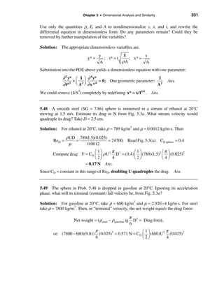
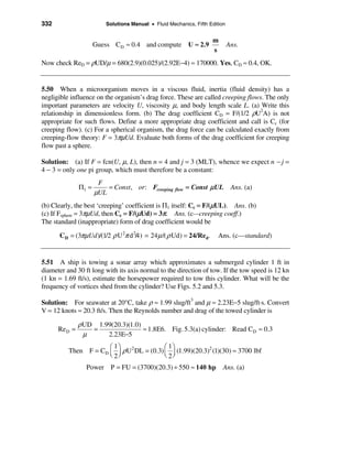
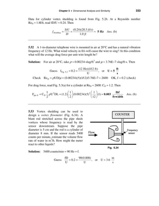
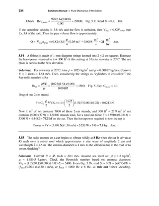
![336 Solutions Manual • Fluid Mechanics, Fifth Edition
This is not an elasticity course, so just use the formula for center deflection of a simply-
supported beam:
FL3 F(0.6)3
δ center = = 0.01 m = , solve for F ≈ 218 N
48EI 48(2.0E11)[(π /4)(0.005)4 ]
ρ 2 æ 1.2 ö 2
Guess CD ≈ 1.2, then F = 218 N = C D V DL = (1.2) ç ÷ V (0.01)(0.6)
2 è 2 ø
Solve for V ≈ 225 m/s, check ReD = ρ VD/µ ≈ 150,000: OK, CD ≈ 1.2 from Fig. 5.3a.
Then V ≈ 225 m/s, which is quite high subsonic speed, Mach number ≈ 0.66. Ans.
5.58 For the steel rod of Prob. 5.57, at what airstream velocity U will the rod begin to
vibrate laterally in resonance in its first mode (a half sine wave)? (Hint: Consult a vibration
text under “lateral beam vibration.”)
Solution: From a vibrations book, the first mode frequency for a simply-supported
slender beam is given by
EI
ωn = π 2 where m = ρsteelπ R 2 = beam mass per unit length
mL4
1/2
ω π é 2.0E11(π /4)(0.005)4 ù
Thus fn = n = ê ú ≈ 55.1 Hz
2π 2 ë (7840)π (0.005)2 (0.6)4 û
The beam will resonate if its vortex shedding frequency is the same. Guess fD/U ≈ 0.2:
fD 55.1(0.01) m
St = ≈ 0.2 = , or U ≈ 2.8
U U s
m
Check Re D = ρ VD/µ ≈ 1800. Fig. 5.2, OK, St ≈ 0.2. Then V ≈ 2.8 Ans.
s
5.59 Modify Prob. 5.55 as follows. If the circular antenna is steel, with L = 60 cm, and the
car speed is 45 mi/h, what rod diameter would cause the natural vibration frequency to equal
the shedding frequency and thus be in a resonant condition?
Solution: For steel take Young’s modulus E = 2.1E11 Pa and ρ = 7840 kg/m3. Look up
the natural frequency of a circular-cross-section elastic cantilever beam and set the two
frequencies equal:
E R 2.1E11 R 0.21(2π U ) 0.21(2π )(20.1)
ω n = 1.758 = 1.758 = ω shed ≈ =
ρ L2
7840 0.6 2
2R 2R](https://image.slidesharecdn.com/solucionariodefluidoswhite-120604143132-phpapp02/85/Solucionario-de-fluidos_white-336-320.jpg)
![340 Solutions Manual • Fluid Mechanics, Fifth Edition
Solution: For steel, E ≈ 29E6 psi ≈ 2.03E11 Pa. If ω = f(M, EI, L), then n = 4 and j = 3
(MLT), hence we get only 1 pi group, which we can evaluate from the steel data:
ω (ML3 )1/2 0.9[(2.0)(0.4)3 ]1/2
= constant = ≈ 0.0224
(EI)1/2 [(2.03E11)(π /4)(0.006)4 ]1/2
For 2024 aluminum, E ≈ 10.6E6 psi ≈ 7.4E10 Pa. Then re-evaluate the same pi group:
ω (ML3 )1/2 ω [(1.0)(0.4)3 ]1/2
New = 0.0224 = , or ω alum ≈ 0.77 Hz Ans.
(EI)1/2 [(7.4E10)(π/4)(0.006)4 ]1/2
5.65 In turbulent flow near a flat wall, the local velocity u varies only with distance y from
the wall, wall shear stress τw, and fluid properties ρ and µ. The following data were taken in the
University of Rhode Island wind tunnel for airflow, ρ = 0.0023 slug/ft3, µ = 3.81E−7 slug/(ft·s),
and τw = 0.029 lbf/ft2:
y, in 0.021 0.035 0.055 0.080 0.12 0.16
u, ft/s 50.6 54.2 57.6 59.7 63.5 65.9
(a) Plot these data in the form of dimensionless u versus dimensionless y, and suggest a
suitable power-law curve fit. (b) Suppose that the tunnel speed is increased until u = 90 ft/s
at y = 0.11 in. Estimate the new wall shear stress, in lbf/ft2.
Solution: Given that u = fcn(y, τw, ρ, µ), then n = 5 and j = 3 (MLT), so we expect
n − j = 5 − 3 = 2 pi groups, and they are traditionally chosen as follows (Chap. 6, Section 6.5):
u æ ρ u*y ö
= fcn ç ÷ , where u* = (τ w / ρ ) = the ‘friction velocity’
1/2
u* è µ ø
We may compute u * = (τw /ρ)1/2 = (0.029/0.0023)1/2 = 3.55 ft/s and then modify the given
data into dimensionless parameters:
y, in: 0.021 0.035 0.055 0.080 0.12 0.16
ρ u * y/µ : 38 63 98 143 214 286
u/u*: 14.3 15.3 16.2 16.8 17.9 18.6
When plotted on log-log paper as follows, they form nearly a straight line:](https://image.slidesharecdn.com/solucionariodefluidoswhite-120604143132-phpapp02/85/Solucionario-de-fluidos_white-340-320.jpg)


![348 Solutions Manual • Fluid Mechanics, Fifth Edition
For seawater, take ρ = 1.99 slug/ft3, µ = 2.23E−5 slug/ft⋅s. With Lp = 150 ft and Vp =
15 knots = 25.3 ft/s, evaluate
ρp Vp L p 1.99(25.3)(150) 25.3
Re proto = = ≈ 3.39E8; Frp = ≈ 0.364
µp 2.23E−5 [32.2(150)]1/2
For Fr ≈ 0.364, interpolate to CF,wave ≈ 0.0027
2 2
Thus we can immediately estimate Fwave ≈ 0.0027(1.99)(25.3) (150) ≈ 77000 lbf. However,
as mentioned in Fig. 5.8 of the text, Rep is far outside the range of the friction force data,
therefore we must extrapolate as best we can. A power-law curve-fit is
0.0178 0.0178
CF,friction ≈ , hence CF,proto ≈ ≈ 0.00105
Re 0.144 (3.39E8)0.144
Thus Ffriction ≈ 0.00105(1.99)(25.3)2(150)2 ≈ 30000 lbf. Ftotal ≈ 107000 lbf. Ans.
5.77 A dam spillway is to be tested by using Froude scaling with a one-thirtieth-scale
model. The model flow has an average velocity of 0.6 m/s and a volume flow of 0.05 m3/s.
What will the velocity and flow of the prototype be? If the measured force on a certain part
of the model is 1.5 N, what will the corresponding force on the prototype be?
Solution: Given α = Lm/Lp = 1/30, Froude scaling requires that
Vm 0.6 m Q 0.05 m3
Vp = = ≈ 3.3 ; Q p = 5m = ≈ 246 Ans. (a)
√α (1/30)1/2 s α /2 (1/30)5/2 s
The force scales in similar manner, assuming that the density remains constant (water):
æ ρ p öæ Vp ö æ Lp ö
2 2 22
æ 1 ö æ1ö
Fp = Fm ç ÷ç ÷ ç ÷ = Fm (1) ç ÷ ç ÷ = (1.5)(30) ≈ 40500 N
3
Ans. (b)
è ρ m øè Vm ø è Lm ø è √α ø è α ø
5.78 A prototype spillway has a characteristic velocity of 3 m/s and a characteristic length
of 10 m. A small model is constructed by using Froude scaling. What is the minimum scale
ratio of the model which will ensure that its minimum Weber number is 100? Both flows
use water at 20°C.
Solution: For water at 20°C, ρ = 998 kg/m3 and Y = 0.073 N/m, for both model and
prototype. Evaluate the Weber number of the prototype:
ρ p Vp L p 998(3.0)2 (10.0)
2
We p = = ≈ 1.23E6; for Froude scaling,
Yp 0.073](https://image.slidesharecdn.com/solucionariodefluidoswhite-120604143132-phpapp02/85/Solucionario-de-fluidos_white-348-320.jpg)

![352 Solutions Manual • Fluid Mechanics, Fifth Edition
µ = 2.92E−4 kg/m·s. For steel take ρ = 7800 kg/m3. Then the net sphere weight in
gasoline is
π 3 π
Wnet = ( ρs − ρ )g D = (7800 − 680)(9.81) (0.025)3 = 0.571 N
6 6
680(0.571)
Fdrag = Wnet , dimensionless force = ρ F/µ 2 = ≈ 4.56E9
(2.92E−4)2
µ Re D (2.92E−4)(2E5) m
Fig. 5.11: read Re D ≈ 2E5, whence V = = ≈3 Ans.
ρD 680(0.025) s
You can’t read the graph any closer than that. We are very near the ‘transition’ point.
5.86 Solve Prob. 5.50, using the modified sphere-drag plot of Fig. 5.11.
Solution: Recall this problem is identical to Prob. 5.85 above except that the fluid is
glycerin, with ρ = 1260 kg/m3 and µ = 1.49 kg/m·s. Evaluate the net weight:
π ρ F 1260(0.525)
W = (7800 − 1260)(9.81) (0.025)3 ≈ 0.525 N, whence 2 = ≈ 298
6 µ (1.49)2
From Fig. 5.11 read Re ≈ 15, or V = 15(1.49)/[1260(0.025)] ≈ 0.7 m/s. Ans.
5.87 In Prob. 5.62 it was difficult to solve
for Ω because it appeared in both power and
flow coefficients. Rescale the problem,
using the data of Fig. P5.61, to make a plot
of dimensionless power versus dimension-
less rotation speed. Enter this plot directly to
solve Prob. 5.62 for Ω.
Fig. P5.61
Solution: Recall that the problem was to find the speed Ω for this pump family if D =
12 cm, Q = 25 m3/hr, and P = 300 W, in gasoline, ρ = 680 kg/m3 and µ = 2.92E−4 kg/m·s.
We can eliminate Ω from the power coefficient for a new type of coefficient:
P Ω3 D9 PD 4 Q
Π3 = ⋅ 3 = , to be plotted versus
ρΩ 3 D 5 Q ρ Q3 ΩD3](https://image.slidesharecdn.com/solucionariodefluidoswhite-120604143132-phpapp02/85/Solucionario-de-fluidos_white-352-320.jpg)
![356 Solutions Manual • Fluid Mechanics, Fifth Edition
Solution: For kerosene at 20°C, take ρ = 804 kg/m3 and µ = 0.00192 kg/m⋅s . We have
to convert correlation “3” in Prob. 5.90 to use the known Q instead of the unknown V.
Substitute Q = (π/4)D2V into both sides of the correlation:
π 2 ∆pD5 0.155 π 2 (220000)D5 0.155 [π (0.00192)D]1/4
≈ , or: ≈
16 ρ Q 2 L (4 ρ Q/πµ D)0.25 16(804)(60/3600)2 (200) [4(804)(60/3600)]1/4
Solve for D 4.75 = 5.25E−6, or D ≈ 0.0774 m Ans.
This looks OK, but check Re = 4ρ Q/(πµD) ≈ 4(804)(60/3600)/[π (0.00192)(0.0774)] ≈
115,000—slightly to the right of the data in Eq. 5.7, Fig. 5.10. Extrapolation is somewhat
risky but in this case gives the correct diameter, whereas the extrapolation in Prob. 5.90
was completely incorrect.](https://image.slidesharecdn.com/solucionariodefluidoswhite-120604143132-phpapp02/85/Solucionario-de-fluidos_white-356-320.jpg)


![362 Solutions Manual • Fluid Mechanics, Fifth Edition
C5.5 Does an automobile radio antenna vibrate in resonance due to vortex shedding?
Consider an antenna of length L and diameter D. According to beam-vibration theory
[e.g. Kelly [34], p. 401], the first mode natural frequency of a solid circular cantilever
beam is ωn = 3.516[EI/(ρAL4)]1/2, where E is the modulus of elasticity, I is the area
moment of inertia, ρ is the beam material density, and A is the beam cross-section area.
(a) Show that ωn is proportional to the antenna radius R. (b) If the antenna is steel, with
L = 60 cm and D = 4 mm, estimate the natural vibration frequency, in Hz. (c) Compare
with the shedding frequency if the car moves at 65 mi/h.
Solution: (a) From Fig. 2.13 for a circular cross-section, A = π R2 and I = π R4/4. Then
the natural frequency is predicted to be:
Eπ R 4 /4 E R
ω n = 3.516 = 1.758 = Const × RP Ans. (a)
ρπ R L
2 4
ρ L2
(b) For steel, E = 2.1E11 Pa and ρ = 7840 kg/m3. If L = 60 cm and D = 4 mm, then
2.1E11 0.002 rad
ω n = 1.758 2
≈ 51 ≈ 8 Hz Ans. (b)
7840 0.6 s
(c) For U = 65 mi/h = 29.1 m/s and sea-level air, check ReD = ρUD/µ = 1.2(29.1)(0.004)/
(0.000018) ≈ 7800. From Fig. 5.2b, read Strouhal number St ≈ 0.21. Then,
ω shed D ω shed (0.004) rad
= ≈ 0.21, or: ω shed ≈ 9600 ≈ 1500 Hz Ans. (c)
2π U 2π (29.1) s
Thus, for a typical antenna, the shedding frequency is far higher than the natural vibration
frequency.](https://image.slidesharecdn.com/solucionariodefluidoswhite-120604143132-phpapp02/85/Solucionario-de-fluidos_white-362-320.jpg)
![364 Solutions Manual • Fluid Mechanics, Fifth Edition
The curve is not quite linear because ν = µ/ρ is not quite linear with T for air in this
range. Ans. (b)
6.3 For a thin wing moving parallel to its chord line, transition to a turbulent boundary
layer occurs at a “local” Reynolds number Rex, where x is the distance from the leading
edge of the wing. The critical Reynolds number depends upon the intensity of turbulent
fluctuations in the stream and equals 2.8E6 if the stream is very quiet. A semiempirical
correlation for this case [Ref. 3 of Ch. 6] is
−1 + (1 + 13.25ζ 2 )1/2
Re1/2 ≈
0.00392ζ 2
xcrit
where ζ is the tunnel-turbulence intensity in percent. If V = 20 m/s in air at 20°C, use this
formula to plot the transition position on the wing versus stream turbulence for ζ between
0 and 2 percent. At what value of ζ is xcrit decreased 50 percent from its value at ζ = 0?
Solution: This problem is merely to illustrate the strong effect of stream turbulence on
the transition point. For air at 20°C, take ρ = 1.2 kg/m3 and µ = 1.8E−5 kg/m⋅s. Compute
Rex,crit from the correlation and plot xtr = µRex/[ρ(20 m/s)] versus percent turbulence:
Fig. P6.3
The value of xcrit decreases by half (to 1.07 meters) at ζ ≈ 0.42%. Ans.](https://image.slidesharecdn.com/solucionariodefluidoswhite-120604143132-phpapp02/85/Solucionario-de-fluidos_white-364-320.jpg)
![Chapter 6 • Viscous Flow in Ducts 365
6.4 For flow of SAE 30 oil through a 5-cm-diameter pipe, from Fig. A.1, for what flow
rate in m3/h would we expect transition to turbulence at (a) 20°C and (b) 100°C?
Solution: For SAE 30 oil take ρ = 891 kg/m 3 and take µ = 0.29 kg/m⋅s at 20°C (Table A.3)
and 0.01 kg/m-s at 100°C (Fig A.1). Write the critical Reynolds number in terms of flow
rate Q:
ρVD 4ρQ 4(891 kg/m3 )Q
(a) Recrit = 2300 = = = ,
µ πµ D π (0.29 kg/m⋅s)(0.05 m)
m3 m3
solve Q = 0.0293 = 106 Ans. (a)
s h
ρVD 4ρQ 4(891 kg/m3 )Q
(b) Re crit = 2300 = = = ,
µ πµ D π (0.010 kg/m⋅s)(0.05 m)
m3 m3
solve Q = 0.00101 = 3.6 Ans. (b)
s h
6.5 In flow past a body or wall, early
transition to turbulence can be induced by
placing a trip wire on the wall across the
flow, as in Fig. P6.5. If the trip wire in
Fig. P6.5 is placed where the local velocity
is U, it will trigger turbulence if Ud/ν = 850,
where d is the wire diameter [Ref. 3 of Ch. 6].
If the sphere diameter is 20 cm and transition
is observed at ReD = 90,000, what is the Fig. P6.5
diameter of the trip wire in mm?
Solution: For the same U and ν,
Ud UD
Re d = = 850; Re D = = 90000,
ν ν
Re æ 850 ö
or d = D d = (200 mm) ç ≈ 1.9 mm
Re D è 90000 ÷
ø
6.6 A fluid at 20°C flows at 850 cm3/s through an 8-cm-diameter pipe. Determine the
entrance length if the fluid is (a) hydrogen; (b) air; (c) gasoline; (d) water; (e) mercury;
and (f) glycerin.
Solution: Tabulate the kinematic viscosities and compute ReD = VD/ν, where V = 4Q/
(πD2) = 4(850E−6 m3/s)/[π (0.08 m)2] = 0.169 m/s. Thus ReD = (0.169)(0.08)/ν = 0.0135/ν.](https://image.slidesharecdn.com/solucionariodefluidoswhite-120604143132-phpapp02/85/Solucionario-de-fluidos_white-365-320.jpg)


![Chapter 6 • Viscous Flow in Ducts 373
Note that “L” in this expression is the tube length only (L = 30 cm).
kg
Solve for µ = 0.00257 (laminar flow) Ans.
m⋅ s
ρVd 948(0.605)(0.002)
Red = = = 446 (laminar )
µ 0.00257
6.19 An oil (SG = 0.9) issues from the
pipe in Fig. P6.19 at Q = 35 ft3/h. What is
the kinematic viscosity of the oil in ft3/s? Is
the flow laminar?
Solution: Apply steady-flow energy:
patm 02 p V2
+ + z1 = atm + 2 + z 2 + h f , Fig. P6.19
ρg 2g ρg 2g
Q 35/3600 ft
where V2 = = ≈ 7.13
A π (0.25 /12) 2
s
2
V2 (7.13)2
Solve h f = z1 − z2 − = 10 − = 9.21 ft
2g 2(32.2)
Assuming laminar pipe flow, use Eq. (6.12) to relate head loss to viscosity:
128ν LQ 128(6)(35/3600)ν µ ft 2
h f = 9.21 ft = = , solve ν = ≈ 3.76E−4 Ans.
π gd 4 π (32.2)(0.5/12)4 ρ s
Check Re = 4Q/(πν d) = 4(35/3600)/[π (3.76E−4)(0.5/12)] ≈ 790 (OK, laminar)
6.20 In Prob. 6.19 what will the flow rate be, in m3/h, if the fluid is SAE 10 oil at 20°C?
Solution: For SAE 10 oil at 20°C, take ρ = 1.69 slug/ft3 and µ =2.17E−3 slug/ft⋅s. The
steady flow energy analysis above gives, for laminar flow,
V2 32µ LV 32(2.17E−3)(6.0)V
h f = 10 − = = = 4.41V (quadratic equation)
2(32.2) ρgd 2 (1.69)(32.2)(0.5/12)2
π æ 0.5 ö
2
ft ft 3 m3
Solve for V ≈ 2.25 , Q = ç ÷ (2.25) = 0.00307 ≈ 0.31 Ans.
s 4 è 12 ø s h](https://image.slidesharecdn.com/solucionariodefluidoswhite-120604143132-phpapp02/85/Solucionario-de-fluidos_white-373-320.jpg)

![376 Solutions Manual • Fluid Mechanics, Fifth Edition
Solution: For water, take ρ = 998 kg/m3 and µ = 0.001 kg/m⋅s. (a) Both tank surfaces
are at atmospheric pressure and have negligible velocity. The energy equation, when
neglecting minor losses, reduces to:
128µ LQ 128(0.001 kg/m⋅s)(3.5 m)Q
∆z = 0.3 m = h f = =
πρgd 4
π (998 kg/m3 )(9.81 m/s2 )(0.004 m)4
m3 m3
Solve for Q = 5.3E−6 = 0.019 Ans. (a)
s h
Check Re d = 4ρQ/(πµ d ) = 4(998)(5.3E−6)/[π (0.001)(0.004)]
Re d = 1675 laminar. Ans. (a)
(b) If Red = 500 = 4ρQ/(πµd) and ∆z = hf, we can solve for both Q and d:
4(998 kg/m3 )Q
Re d = 500 = , or Q = 0.000394d
π (0.001 kg/m⋅s)d
128(0.001 kg/m⋅s)(3.5 m)Q
h f = 0.3 m = , or Q = 20600d 4
π (998 kg/m3 )(9.81 m/s2 )d 4
Combine these two to solve for Q = 1.05E−6 m 3 /s and d = 2.67 mm Ans. (b)
6.25 For the configuration shown in
Fig. P6.25, the fluid is ethyl alcohol at
20°C, and the tanks are very wide. Find the
flow rate which occurs in m3/h. Is the flow
laminar?
Solution: For ethanol, take ρ =
789 kg/m3 and µ = 0.0012 kg/m⋅s. Write
the energy equation from upper free
surface (1) to lower free surface (2): Fig. P6.25
p1 V12 p 2
V2
+ + z1 = 2 + + z + h , with p1 = p2 and V1 ≈ V2 ≈ 0
ρg 2g ρg 2g 2 f
128µ LQ 128(0.0012)(1.2 m)Q
Then h f = z1 − z 2 = 0.9 m = =
πρgd 4 π (789)(9.81)(0.002)4
Solve for Q ≈ 1.90E−6 m 3 /s = 0.00684 m 3 /h. Ans.
Check the Reynolds number Re = 4ρQ/(πµd) ≈ 795 − OK, laminar flow.](https://image.slidesharecdn.com/solucionariodefluidoswhite-120604143132-phpapp02/85/Solucionario-de-fluidos_white-376-320.jpg)


![Chapter 6 • Viscous Flow in Ducts 379
6.30 SAE 10 oil at 20°C flows through
the 4-cm-diameter vertical pipe of
Fig. P6.30. For the mercury manometer
reading h = 42 cm shown, (a) calculate the
volume flow rate in m3/h, and (b) state the
direction of flow.
Solution: For SAE 10 oil, take ρ =
870 kg/m3 and µ = 0.104 kg/m⋅s. The
pressure at the lower point (1) is
considerably higher than p2 according to the Fig. P6.30
manometer reading:
p1 − p2 = ( ρHg − ρ oil )g∆h = (13550 − 870)(9.81)(0.42) ≈ 52200 Pa
∆p/(ρoil g) = 52200/[870(9.81)] ≈ 6.12 m
This is more than 3 m of oil, therefore it must include a friction loss: flow is up. Ans. (b)
The energy equation between (1) and (2), with V1 = V2, gives
p1 − p 2 128µ LQ
= z 2 − z1 + h f , or 6.12 m = 3 m + h f , or: h f ≈ 3.12 m =
ρg πρ gd 4
(6.12 − 3)π (870)(9.81)(0.04)4 m3 m3
Compute Q = = 0.00536 ≈ 19.3 Ans. (a)
128(0.104)(3.0) s h
Check Re = 4ρQ/(πµd) = 4(870)(0.00536)/[π (0.104)(0.04)] ≈ 1430 (OK, laminar flow).
6.31 Light oil, ρ = 880 kg/m3 and µ = 0.015 kg/(m⋅s), flows down a vertical 6-mm-
diameter tube due to gravity only. Estimate the volume flow rate in m3/h if (a) L = 1 m
and (b) L = 2 m. (c) Verify that the flow is laminar.
Solution: If the flow is due to gravity only, the head loss matches the elevation change:
128µ LQ πρ gd 4
h f = ∆z = L = , or Q = independent of pipe length
πρ gd 4 128µ
For this case,
m3 m3
Q = π (880)(9.81)(0.006) /[128(0.015)] ≈ 1.83E−5
4
= 0.066 Ans. (a, b)
s h
Check Re = 4ρQ/(πµd) = 4(880)(1.83E−5)/[π (0.015)(0.006)] ≈ 228 (laminar). Ans. (c)](https://image.slidesharecdn.com/solucionariodefluidoswhite-120604143132-phpapp02/85/Solucionario-de-fluidos_white-379-320.jpg)

![Chapter 6 • Viscous Flow in Ducts 381
Solution: For SAE 30 oil at 20°C, ρ = 891 kg/m3 and µ = 0.29 kg/m⋅s. With mass flow
known, we can evaluate the pipe velocity:
m& 3 kg/s m
V= = = 4.76 ,
ρ A 891π (0.015) 2
s
891(4.76)(0.03)
Check Red = = 439 (OK, laminar )
0.29
Apply the steady flow energy equation between A and B:
2
pA VA p V2 500000 180000
+ + z A = B + B + zB + h f − hp , or: = + 15 + h f − hp
ρ g 2g ρ g 2g 891(9.81) 891(9.81)
32µ LV 32(0.29)(25)(4.76)
where h f = = = 140.5 m, Solve for hpump = 118.9 m
ρgd 2 891(9.81)(0.03)2
The pump power is then given by
æ kg ö æ mö
Power = ρ gQhp = mghp = ç 3
& ÷ ç 9.81 2 ÷ (118.9 m) = 3500 watts Ans.
è s øè s ø
6.34 Derive the time-averaged x-momentum equation (6.21) by direct substitution of
Eqs. (6.19) into the momentum equation (6.14). It is convenient to write the convective
acceleration as
du ∂ 2 ∂ ∂
= (u ) + (uv) + (uw)
dt ∂ x ∂y ∂z
which is valid because of the continuity relation, Eq. (6.14).
Solution: Into the x-momentum eqn. substitute u = u + u’, v = v + v’, etc., to obtain
é∂ ∂ ∂ ù
ρ ê (u 2 + 2uu’ + u’2 ) + (v u + vu’ + v’u + v’u’) + (wu + wu’ + w’u + w’u’)ú
ë∂x ∂y ∂z û
∂
= − (p + p’) + ρg x + µ[∇2 (u + u’)]
∂x
Now take the time-average of the entire equation to obtain Eq. (6.21) of the text:
é du ∂ ∂ ∂ ù ∂p
ρê + ( u’2 ) + ( u’v’) + ( u’w’) ú = − + ρ g x + µ∇ 2 ( u ) Ans.
ë dt ∂ x ∂y ∂z û ∂x](https://image.slidesharecdn.com/solucionariodefluidoswhite-120604143132-phpapp02/85/Solucionario-de-fluidos_white-381-320.jpg)


![Chapter 6 • Viscous Flow in Ducts 385
6.40 Theodore von Kármán in 1930 theorized that turbulent shear could be represented
by τ turb = ε du/dy where ε = ρκ 2y2du/dy is called the mixing-length eddy viscosity and κ ≈
0.41 is Kármán’s dimensionless mixing-length constant [2,3]. Assuming that τ turb ≈ τw
near the wall, show that this expression can be integrated to yield the logarithmic-overlap
law, Eq. (6.28).
Solution: This is accomplished by straight substitution:
du é 2 2 du ù du du u*
τ turb ≈ τ w = ρu*2 = ε = ê ρκ y ú , solve for =
dy ë dy û dy dy κ y
u* dy u*
Integrate: ò du = κ ò y
, or: u =
κ
ln(y) + constant Ans.
To convert this to the exact form of Eq. (6.28) requires fitting to experimental data.
6.41 Water at 20°C flows in a 9-cm-diameter pipe under fully developed conditions.
The centerline velocity is 10 m/s. Compute (a) Q, (b) V, (c) τw, and (d) ∆p for a 100-m
pipe length.
Solution: For water at 20°C, take ρ = 998 kg/m3 and µ = 0.001 kg/m⋅s. Check Re =
ρVD/µ ≈ 998(10)(0.09)/0.001 ≈ 900,000, surely a turbulent flow. Use the log-law:
u ctr 1 æ Ru* ö 10 1 é 998(0.045)u* ù m
≈ ln ç ÷ + B, or: ≈ ln ê ú + 5.0, solve u* ≈ 0.350 s
u* κ è ν ø u* 0.41 ë 0.001 û
Then τ w = ρu*2 = (998)(0.350)2 ≈ 122 Pa Ans. (c)
We know that average velocity V is slightly less than centerline velocity, but we probably
wouldn’t know at this stage the formula for V from Eq. (6.43). So just make an estimate:
m
V ≈ 0.85u ctr = (0.85)(10) ≈ 8.5 Ans. (b)
s
Q = AV ≈ (π /4)(0.09)2 (8.5) ≈ 0.054 m 3 /s Ans. (a)
Finally, assuming fully-developed horizontal flow, we use Eq. (6.9b) to compute ∆p:
2τ w ∆L 2(122 Pa)(100 m)
∆p = = ≈ 542, 000 Pa Ans. (d)
R (0.045 m)](https://image.slidesharecdn.com/solucionariodefluidoswhite-120604143132-phpapp02/85/Solucionario-de-fluidos_white-385-320.jpg)

![Chapter 6 • Viscous Flow in Ducts 387
With f known, we compute the head loss and (horizontal) pressure drop as
L V2 æ 5280 ö 1(11.35)2
hf = f = (0.0189) ç ÷ ≈ 800 ft Ans. (a)
d 2g è 3/12 ø 2(32.2)
lbf
and ∆p = ρ gh f = (1.94)(32.2)(800) ≈ 49900 Ans. (b)
ft 2
6.44 Mercury at 20°C flows through 4 meters of 7-mm-diameter glass tubing at an
average velocity of 5 m/s. Estimate the head loss in meters and the pressure drop in kPa.
Solution: For mercury at 20°C, take ρ = 13550 kg/m3 and µ = 0.00156 kg/m⋅s. Glass
tubing is considered hydraulically “smooth,” ε/d = 0. Compute the Reynolds number:
ρVd 13550(5)(0.007)
Red = = = 304,000; Moody chart smooth: f ≈ 0.0143
µ 0.00156
L V2 æ 4.0 ö 5
2
hf = f = 0.0143 ç ÷ = 10.4 m Ans. (a)
d 2g è 0.007 ø 2(9.81)
∆p = ρ gh f = (13550)(9.81)(10.4) = 1,380,000 Pa = 1380 kPa Ans. (b)
6.45 Oil, SG = 0.88 and ν = 4E−5 m2/s, flows at 400 gal/min through a 6-inch asphalted
cast-iron pipe. The pipe is 0.5 miles long (2640 ft) and slopes upward at 8° in the flow
direction. Compute the head loss in feet and the pressure change.
Solution: First convert 400 gal/min = 0.891 ft3/s and ν = 0.000431 ft2/s. For asphalted
cast-iron, ε = 0.0004 ft, hence ε/d = 0.0004/0.5 = 0.0008. Compute V, Red, and f:
0.891 ft 4.54(0.5)
V= = 4.54 ; Red = = 5271; calculate f Moody = 0.0377
π (0.25) 2
s 0.000431
L V2 æ 2640 ö (4.54)
2
then h f = f = 0.0377 ç = 63.8 ft Ans. (a)
d 2g è 0.5 ÷ 2(32.2)
ø
If the pipe slopes upward at 8°, the pressure drop must balance both friction and gravity:
lbf
∆p = ρg(h f + ∆z ) = 0.88(62.4)[63.8 + 2640sin 8°] = 23700 Ans. (b)
ft 2](https://image.slidesharecdn.com/solucionariodefluidoswhite-120604143132-phpapp02/85/Solucionario-de-fluidos_white-387-320.jpg)
![390 Solutions Manual • Fluid Mechanics, Fifth Edition
6.50 Ethanol at 20°C flows at 125 U.S. gal/min through a horizontal cast-iron pipe with
L = 12 m and d = 5 cm. Neglecting entrance effects, estimate (a) the pressure gradient, dp/dx;
(b) the wall shear stress, τw; and (c) the percent reduction in friction factor if the pipe
walls are polished to a smooth surface.
Solution: For ethanol (Table A-3) take ρ = 789 kg/m3 and µ = 0.0012 kg/m⋅s. Convert
125 gal/min to 0.00789 m3/s. Evaluate V = Q/A = 0.00789/[π (0.05)2/4] = 4.02 m/s.
ρVd 789(4.02)(0.05) ε 0.26 mm
Red = = = 132,000, = = 0.0052 Then f Moody ≈ 0.0314
µ 0.0012 d 50 mm
f 0.0314
(b) τ w = ρV 2 = (789)(4.02)2 = 50 Pa Ans. (b)
8 8
dp 4τ w −4(50) Pa
(a) =− = = −4000 Ans. (a)
dx d 0.05 m
(c) Re = 132000, fsmooth = 0.0170, hence the reduction in f is
æ 0.0170 ö
ç1 −
è 0.0314 ÷
ø
= 46% Ans. (c)
6.51 The viscous sublayer (Fig. 6.10) is normally less than 1 percent of the pipe
diameter and therefore very difficult to probe with a finite-sized instrument. In an effort
to generate a thick sublayer for probing, Pennsylvania State University in 1964 built a
pipe with a flow of glycerin. Assume a smooth 12-in-diameter pipe with V = 60 ft/s and
glycerin at 20°C. Compute the sublayer thickness in inches and the pumping horsepower
required at 75 percent efficiency if L = 40 ft.
Solution: For glycerin at 20°C, take ρ = 2.44 slug/ft3 and µ = 0.0311 slug/ft⋅s. Then
ρVd 2.44(60)(1 ft)
Re = = = 4710 (barely turbulent!) Smooth: fMoody ≈ 0.0380
µ 0.0311
1/2
æ 0.0380 ö ft
Then u* = V(f/8)1/2 = 60 ç ≈ 4.13
è 8 ÷ ø s
The sublayer thickness is defined by y+ ≈ 5.0 = ρyu*/µ. Thus
5µ 5(0.0311)
ysublayer ≈ = = 0.0154 ft ≈ 0.185 inches Ans.
ρ u* (2.44)(4.13)](https://image.slidesharecdn.com/solucionariodefluidoswhite-120604143132-phpapp02/85/Solucionario-de-fluidos_white-390-320.jpg)
![Chapter 6 • Viscous Flow in Ducts 391
With f known, the head loss and the power required can be computed:
L V2 æ 40 ö (60)
2
hf = f = (0.0380) ç ÷ ≈ 85 ft
d 2g è 1 ø 2(32.2)
ρ gQh f 1 éπ ù
P= = (2.44)(32.2) ê (1)2 (60) ú (85) = 419000 ÷ 550 ≈ 760 hp Ans.
η 0.75 ë4 û
6.52 The pipe flow in Fig. P6.52 is driven
by pressurized air in the tank. What gage
pressure p1 is needed to provide a 20°C
water flow rate Q = 60 m3/h?
Solution: For water at 20°C, take ρ =
998 kg/m3 and µ = 0.001 kg/m⋅s. Get V,
Re, f:
60/3600 m
V= = 8.49 ;
(π /4)(0.05)2 s Fig. P6.52
998(8.49)(0.05)
Re = ≈ 424000; fsmooth ≈ 0.0136
0.001
Write the energy equation between points (1) (the tank) and (2) (the open jet):
2
p1 02 0 Vpipe L V2 m
+ + 10 = + + 80 + h f , where h f = f and Vpipe = 8.49
ρg 2g ρg 2g d 2g s
é (8.49)2 ì æ 170 ö ü ù
Solve p1 = (998)(9.81) ê80 − 10 + í1 + 0.0136 ç ý
ë 2(9.81) î è 0.05 ÷ þ ú
ø û
≈ 2.38E6 Pa Ans.
[This is a gage pressure (relative to the pressure surrounding the open jet.)]
6.53 In Fig. P6.52 suppose p1 = 700 kPa and the fluid specific gravity is 0.68. If the
flow rate is 27 m3/h, estimate the viscosity of the fluid. What fluid in Table A-5 is the
likely suspect?](https://image.slidesharecdn.com/solucionariodefluidoswhite-120604143132-phpapp02/85/Solucionario-de-fluidos_white-391-320.jpg)
![392 Solutions Manual • Fluid Mechanics, Fifth Edition
Solution: Evaluate ρ = 0.68(998) = 679 kg/m3. Evaluate V = Q/A = (27/3600)/[π (0.025)2] =
3.82 m/s. The energy analysis of the previous problem now has f as the unknown:
p1 700000 V2 L V2 (3.82)2 é 170 ù
= = ∆z + +f = 70 + ê1 + f 0.05 ú , solve f = 0.0136
ρg 679(9.81) 2g d 2g 2(9.81) ë û
679(3.82)(0.05)
Smooth pipe: f = 0.0136, Red = 416000 = ,
µ
kg
Solve µ = 0.00031 Ans.
m⋅ s
The density and viscosity are close to the likely suspect, gasoline. Ans.
6.54* A swimming pool W by Y by h deep is to be emptied by gravity through the long
pipe shown in Fig. P6.54. Assuming an average pipe friction factor fav and neglecting
minor losses, derive a formula for the time to empty the tank from an initial level ho.
Fig. P6.54
Solution: With no driving pressure and negligible tank surface velocity, the energy
equation can be combined with a control-volume mass conservation:
V2 L V2 π 2 gh dh
h( t ) = + fav , or: Qout = ApipeV = D 2 = −WY
2g D 2g 4 1 + fav L/D dt
We can separate the variables and integrate for time to drain:
π 2
( )
t 0
2g dh
4
D ò dt = −WY ò h = −WY 0 − 2 ho
1 + fav L/D 0 ho
1/2
4WY 2 ho (1 + fav L/ D)
Clean this up to obtain: tdrain ≈ Ans.
π D2 g](https://image.slidesharecdn.com/solucionariodefluidoswhite-120604143132-phpapp02/85/Solucionario-de-fluidos_white-392-320.jpg)
![394 Solutions Manual • Fluid Mechanics, Fifth Edition
Relating the known pressure drop to friction factor yields the unknown pipe length:
Lρ 2 L æ 910 ö
∆p = 8,000,00 − 400,000 Pa = f V = 0.0157 ç
2
÷ (2.63) ,
d 2 1.22 è 2 ø
Solve L = 188, 000 m = 117 miles Ans. (a)
The pumping power required follows from the pressure drop and flow rate:
Q ∆p 3.07(8 E 6 − 4 E 5)
Power = = = 2.65E 7 watts
Efficiency 0.88
= 26.5 MW (35,500 hp) Ans. (b)
6.57 Apply the analysis of Prob. 6.54 to the following data. Let W = 5 m, Y = 8 m, ho =
2 m, L = 15 m, D = 5 cm, and ε = 0. (a) By letting h = 1.5 m and 0.5 m as representative
depths, estimate the average friction factor. Then (b) estimate the time to drain the pool.
Solution: For water, take ρ = 998 kg/m3 and µ = 0.001 kg/m⋅s. The velocity in Prob. 6.54
is calculated from the energy equation:
2 gh ρVD
V= with f = fcn(Re D )smooth pipe and Re D = , L/D = 300
1 + fL/D µ
(a) With a bit of iteration for the Moody chart, we obtain ReD = 108,000 and f ≈
0.0177 at h = 1.5 m, and ReD = 59,000 and f ≈ .0202 at h = 0.5 m; thus the average
value fav ≈ 0.019. Ans. (a)
The drain formula from Prob. 6.54 then predicts:
4WY 2ho (1 + fav L/D) 4(5)(8) 2(2)[1 + 0.019(300)]
t drain ≈ ≈
π D2 g π (0.05)2 9.81
= 33700 s = 9.4 h Ans. (b)
6.58 In Fig. P6.55 assume that the pipe is
cast iron with L = 550 m, d = 7 cm, and ∆z =
100 m. If an 80 percent efficient pump is
placed at point B, what input power is
required to deliver 160 m3/h of water upward
from reservoir 2 to 1?
Fig. P6.55](https://image.slidesharecdn.com/solucionariodefluidoswhite-120604143132-phpapp02/85/Solucionario-de-fluidos_white-394-320.jpg)


![Chapter 6 • Viscous Flow in Ducts 401
We simply plot Reynolds number versus ζ for various ε/d, as shown below:
To solve Example 6.9, a 100-m-long, 30-cm-diameter pipe with a head loss of 8 m and
ε/d = 0.0002, we use that data to compute ζ = 5.3E7. The oil properties are ρ = 950 kg/m3
and ν = 2E−5 m2/s. Enter the chart above: let’s face it, the scale is very hard to read, but
we estimate, at ζ = 5.3E7, that 6E4 < Red < 9E4, which translates to a flow rate of
0.28 < Q < 0.42 m3/s. Ans. (Example 6.9 gave Q = 0.342 m3/s.)
6.69 For Prob. 6.62 suppose the only pump available can deliver only 80 hp to the fluid.
What is the proper pipe size in inches to maintain the 3 ft3/s flow rate?
Solution: For water at 20°C, take ρ = 1.94 slug/ft3 and µ = 2.09E−5 slug/ft⋅s. For cast
iron, take ε ≈ 0.00085 ft. We can’t specify ε/d because we don’t know d. The energy analysis
above is correct and should be modified to replace V by Q:
L (4Q/π d 2 )2 2000 [4(3.0)/π d2 ]2 f
h p = 120 + f = 120 + f = 120 + 453 5
d 2g d 2(32.2) d
Power 80(550) 453 f
But also h p = = = 235 = 120 + 5 , or: d 5 ≈ 3.94f
ρgQ 62.4(3.0) d](https://image.slidesharecdn.com/solucionariodefluidoswhite-120604143132-phpapp02/85/Solucionario-de-fluidos_white-401-320.jpg)
![402 Solutions Manual • Fluid Mechanics, Fifth Edition
Guess f ≈ 0.02, calculate d, ε/d and Re and get a better f and iterate:
4 ρQ 4(1.94)(3.0)
f ≈ 0.020, d ≈ [3.94(0.02)]1/5 ≈ 0.602 ft, Re = = ,
πµd π (2.09E−5)(0.602)
ε 0.00085
or Re ≈ 589000, = ≈ 0.00141, Moody chart: fbetter ≈ 0.0218 (repeat)
d 0.602
We are nearly converged. The final solution is f ≈ 0.0217, d ≈ 0.612 ft ≈ 7.3 in Ans.
6.70 In Prob. 6.62 suppose the pipe is 6-inch-diameter cast iron and the pump delivers
75 hp to the flow. What flow rate Q in ft3/s results?
Solution: For water at 20°C, take ρ = 1.94 slug/ft3 and µ = 2.09E−5 slug/ft⋅s. For cast
iron, take ε ≈ 0.00085 ft, or ε/d = 0.00085/(6/12) ≈ 0.0017. The energy analysis holds:
ì æ 2000 ö [4Q/π (6/12)2 ]2 ü ft⋅lbf
Power = ρgQh p = 62.4Q í120 + f ç ÷ ý = 75(550)
î è 6/12 ø 2(32.2) ï
þ s
Clean up: 661 ≈ Q(120 + 1611Q 2 f), solve by iteration using ε /d and Re
Guess f ≈ 0.02, Q ≈ 2.29 ft 3 /s, Re = 4 ρQ/πµd ≈ 541000, then fbetter ≈ 0.0228
Convergence is near: f ≈ 0.02284, Re ≈ 522000, Q ≈ 2.21 ft 3 /s. Ans.
6.71 It is desired to solve Prob. 6.62 for the most economical pump and cast-iron pipe
system. If the pump costs $125 per horsepower delivered to the fluid and the pipe costs
$7000 per inch of diameter, what are the minimum cost and the pipe and pump size to
maintain the 3 ft3/s flow rate? Make some simplifying assumptions.
Solution: For water at 20°C, take ρ = 1.94 slug/ft3 and µ = 2.09E−5 slug/ft⋅s. For cast
iron, take ε ≈ 0.00085 ft. Write the energy equation (from Prob. 6.62) in terms of Q and d:
ρgQ 62.4(3.0) ì æ 2000 ö [4(3.0)/π d ] ü
2 2
154.2f
Pin hp = (∆z + h f ) = í120 + f ç ÷ ý = 40.84 +
550 550 î è d ø 2(32.2) ï þ d5
Cost = $125Php + $7000d inches = 125(40.84 + 154.2f/d 5 ) + 7000(12d), with d in ft.
Clean up: Cost ≈ $5105 + 19278f/d 5 + 84000d](https://image.slidesharecdn.com/solucionariodefluidoswhite-120604143132-phpapp02/85/Solucionario-de-fluidos_white-402-320.jpg)
![Chapter 6 • Viscous Flow in Ducts 403
Regardless of the (unknown) value of f, this Cost relation does show a minimum. If we
assume for simplicity that f is constant, we may use the differential calculus:
d(Cost)
|f ≈const = −5(19278)f + 84000, or d best ≈ (1.148 f)1/6
d(d ) d6
4 ρQ ε
Guess f ≈ 0.02, d ≈ [1.148(0.02)]1/6 ≈ 0.533 ft, Re = ≈ 665000, ≈ 0.00159
πµd d
Then fbetter ≈ 0.0224, d better ≈ 0.543 ft (converged)
Result: dbest ≈ 0.543 ft ≈ 6.5 in, Costmin ≈ $14300pump + $45600pipe ≈ $60000. Ans.
6.72 Modify Prob. P6.57 by letting the diameter be unknown. Find the proper pipe
diameter for which the pool will drain in about 2 hours flat.
Solution: Recall the data: Let W = 5 m, Y = 8 m, ho = 2 m, L = 15 m, and ε = 0, with
water, ρ = 998 kg/m3 and µ = 0.001 kg/m⋅s. We apply the same theory as Prob. 6.57:
2 gh 4WY 2ho (1 + fav L/D)
V= , t drain ≈ , fav = fcn(Re D ) for a smooth pipe.
1 + fL/D π D2 g
For the present problem, tdrain = 2 hours and D is the unknown. Use an average value h =
1 m to find fav. Enter these equations on EES (or you can iterate by hand) and the final
results are
V = 2.36 m/s; Re D = 217,000; fav ≈ 0.0154; D = 0.092 m ≈ 9.2 cm Ans.
6.73 The Moody chart, Fig. 6.13, is best for finding head loss (or ∆p) when Q, V, d, and L
are known. It is awkward for the “3rd” type of problem, finding d when hf (or ∆p) and Q
are known (see Ex. 6.11). Prepare a modified Moody chart whose abscissa is independent
of d, using as a parameter ε non-dimensionalized without d, from which one can
immediately read the (dimensionless) ordinate to find d. Use your chart to solve Ex. 6.11.
Solution: An appropriate Pi group which does not contain d is β = (ghfQ3)/(Lν5).
Similarly, an appropriate roughness parameter without d is σ = (εν/Q). After a lot of
algebra, the Colebrook friction factor formula (6.48) becomes
æ 128β ö
1/2
é πσ Red 2.51Red ù
3/2
5/2
Red = −2.0 ç 3 ÷ log10 ê + ú
è π ø ë 14.8 (128β /π 3 )1/2 û](https://image.slidesharecdn.com/solucionariodefluidoswhite-120604143132-phpapp02/85/Solucionario-de-fluidos_white-403-320.jpg)
![404 Solutions Manual • Fluid Mechanics, Fifth Edition
A plot of this messy relation is given below.
To solve Example 6.11, a 100-m-long, unknown-diameter pipe with a head loss of 8 m,
flow rate of 0.342 m3/s, and ε = 0.06 mm, we use that data to compute β = 9.8E21 and
σ = 3.5E−6. The oil properties are ρ = 950 kg/m3 and ν = 2E−5 m2/s. Enter the chart
above: let’s face it, the scale is very hard to read, but we estimate, at β = 9.8E21 and σ =
3.5E−6, that 6E4 < Red < 8E4, which translates to a diameter of 0.27 < d < 0.36 m. Ans.
(Example 6.11 gave d = 0.3 m.)
6.74 In Fig. P6.67 suppose the fluid is gasoline at 20°C and h = 90 ft. What
commercial-steel pipe diameter is required for the flow rate to be 0.015 ft3/s?
Solution: For commercial steel, take ε ≈ 0.00015 ft. For gasoline, take ρ = 1.32 slug/ft3
and µ = 6.1E−6 slug/ft⋅s. From Prob. 6.61 the energy relation gives
V2 (4Q/π d2 )2 æ Lö [4(0.015)/π d2 ]2 ì 80 ü
h= + hf = ç 1 + f ÷ , or: 90 ft = í1 + f ý
2g 2g è dø 2(32.2) î dþ
ε 0.00015
Clean up: d ≈ 0.0158(1 + 80f/d)1/4 with f determined from Re and =
d d
Because d appears implicitly in two places, considerable iteration is required:
Guess f ≈ 0.02, d ≈ 0.0158[1 + 80(0.02)/d]1/4 ≈ 0.0401 ft,
4 ρQ 4(1.32)(0.015) ε
Re = = ≈ 103000, ≈ 0.00374, fbetter ≈ 0.0290
πµd π (6.1E−6)(0.0401) d
Converges to f ≈ 0.0290, Re ≈ 96000, d ≈ 0.0431 ft ≈ 0.52 inches Ans.](https://image.slidesharecdn.com/solucionariodefluidoswhite-120604143132-phpapp02/85/Solucionario-de-fluidos_white-404-320.jpg)
![Chapter 6 • Viscous Flow in Ducts 411
ε ≈ 0.26 mm, hence ε/d = 0.26/(1000d) with d unknown. Head loss must match pump
head:
8fLQ 2 8f(95)(0.7)2 3.85f
hf = = 2 = 5 = h pump ≈ 80 − 20Q 2 = 80 − 20(0.7)2 ≈ 70.2 m,
π gd
2 5
π (9.81)d 5
d
or: d ≈ 0.559f 1/5 . Guess f ≈ 0.02, d ≈ 0.559(0.02)1/5 ≈ 0.256 m
Re = 4 ρQ/(πµd) ≈ 4.61E6, ε /d = 0.26/[1000(0.2560] ≈ 0.00102
Keep iterating: fbetter ≈ 0.0198, dbetter ≈ 0.255 m, Rebetter ≈ 4.62E6, ε/d|better ≈ 0.00102, etc.
The process converges to f ≈ 0.0198, d ≈ 0.255 m. Ans.
6.86 SAE 10 oil at 20°C flows at an average velocity of 2 m/s between two smooth
parallel horizontal plates 3 cm apart. Estimate (a) the centerline velocity, (b) the head loss
per meter, and (c) the pressure drop per meter.
Solution: For SAE 10 oil, take ρ = 870 kg/m3 and µ = 0.104 kg/m⋅s. The half-distance
between plates is called “h” (see Fig. 6.37). Check Dh and Re:
4A ρVD h 870(2.0)(0.06)
Dh = = 4h = 6 cm, Re Dh = = ≈ 1004 (laminar)
P µ 0.104
3 3
Then uCL = u max = V = (2.0) ≈ 3.0 m/s Ans. (a)
2 2
The head loss and pressure drop per meter folow from laminar theory, Eq. (6.63):
3µ VL 3(0.104)(2.0)(1.0)
∆p = = ≈ 2770 Pa/m Ans. (c)
h2 (0.015 m)2
∆p 2770
hf = = ≈ 0.325 m/m Ans. (b)
ρ g 870(9.81)
6.87 A commercial-steel annulus 40 ft long, with a = 1 in and b = 1 in, connects two
2
reservoirs which differ in surface height by 20 ft. Compute the flow rate in ft3/s through
the annulus if the fluid is water at 20°C.](https://image.slidesharecdn.com/solucionariodefluidoswhite-120604143132-phpapp02/85/Solucionario-de-fluidos_white-411-320.jpg)
![Chapter 6 • Viscous Flow in Ducts 413
where h is the half-thickness between plates. If there are N passages, then b = 50 cm for
all and h = 0.5 m/(2N). We find h and N such that NQ = 900 m3/h for the full set of
passages. The problem is ideal for EES, but one can iterate with a calculator also. We
find that 18 passages are one too many—Q only equals 835 m3/h. The better solution is:
N = 17 passages, QN = 935 m 3 /h, h = 1.47 cm, Re Dh = 512 (laminar flow)
6.89 An annulus of narrow clearance causes a very large pressure drop and is useful as
an accurate measurement of viscosity. If a smooth annulus 1 m long with a = 50 mm and
b = 49 mm carries an oil flow at 0.001 m3/s, what is the oil viscosity if the pressure drop
is 250 kPa?
Solution: Assuming laminar flow, use Eq. (6.73) for the pressure drop and flow rate:
π ∆p é 4 4 (a 2 − b2 )2 ù
Q= êa − b − ú , or, for the given data:
8µ L ë ln(a/b) û
π æ 250000 ö é {(0.05)2 − (0.049)2 }2 ù
0.001 m 3 /s = ç ÷ê (0.05)4 − (0.049)4 − ú
8µ è 1 m ø ë ln(0.05/0.049) û
Solve for µ ≈ 0.0065 kg/m⋅ s Ans.
6.90 A 90-ft-long sheet-steel duct carries
air at approximately 20°C and 1 atm. The
duct cross section is an equilateral triangle
whose side measures 9 in. If a blower can
supply 1 hp to the flow, what flow rate, in
ft3/s, will result? Fig. P6.90
Solution: For air at 20°C and 1 atm, take ρ ≈ 0.00234 slug/ft3 and µ = 3.76E−7 slug/ft⋅s.
Compute the hydraulic diameter, and express the head loss in terms of Q:
4A 4(1/2)(9)(9 sin 60°)
Dh = = = 5.2 ′′ = 0.433 ft
P 3(9)
L (Q/A)2 æ 90 ö {Q/[0.5(9/12) sin 60°]}
2 2
hf = f = fç ≈ 54.4fQ 2
D h 2g è 0.433 ÷
ø 2(32.2)](https://image.slidesharecdn.com/solucionariodefluidoswhite-120604143132-phpapp02/85/Solucionario-de-fluidos_white-413-320.jpg)
![414 Solutions Manual • Fluid Mechanics, Fifth Edition
For sheet steel, take ε ≈ 0.00015 ft, hence ε/Dh ≈ 0.000346. Now relate everything to the
input power:
ft⋅lbf
Power = 1 hp = 550 = ρgQh f = (0.00234)(32.2)Q[54.4fQ 2 ],
s
or: fQ3 ≈ 134 with Q in ft 3 /s
ft 3 ρ(Q/A)D h
Guess f ≈ 0.02, Q = (134/0.02) 1/3
≈ 18.9 , Re = ≈ 209000
s µ
Iterate: fbetter ≈ 0.0179, Qbetter ≈ 19.6 ft3/s, Rebetter ≈ 216500. The process converges to
f ≈ 0.01784, V ≈ 80.4 ft/s, Q ≈ 19.6 ft3/s. Ans.
6.91 Heat exchangers often consist of
many triangular passages. Typical is Fig.
P6.91, with L = 60 cm and an isosceles-
triangle cross section of side length a =
2 cm and included angle β = 80°. If the
average velocity is V = 2 m/s and the fluid
is SAE 10 oil at 20°C, estimate the
pressure drop. Fig. P6.91
Solution: For SAE 10 oil, take ρ = 870 kg/m3 and µ = 0.104 kg/m⋅s. The Reynolds
number based on side length a is Re = ρVa/µ ≈ 335, so the flow is laminar. The bottom
side of the triangle is 2(2 cm)sin40° ≈ 2.57 cm. Calculate hydraulic diameter:
1 4A
A= (2.57)(2 cos 40°) ≈ 1.97 cm 2 ; P = 6.57 cm; D h = ≈ 1.20 cm
2 P
ρVD h 870(2.0)(0.0120)
Re Dh = = ≈ 201; from Table 6.4, θ = 40°, fRe ≈ 52.9
µ 0.104
52.9 L ρ 2 æ 0.6 ö æ 870 ö 2
Then f = ≈ 0.263, ∆p = f V = (0.263) ç
è 0.012 ÷ ç 2 ÷
(2)
201 Dh 2 øè ø
≈ 23000 Pa Ans.](https://image.slidesharecdn.com/solucionariodefluidoswhite-120604143132-phpapp02/85/Solucionario-de-fluidos_white-414-320.jpg)

![416 Solutions Manual • Fluid Mechanics, Fifth Edition
Solution: For SAE 10 oil, take ρ = 870 kg/m3 and µ = 0.104 kg/m⋅s. This problem can
be done by hand but would benefit from a computer program. Note that, for arbitrary β,
1 a2 4A a sinβ β
A= (a sin θ )(2a cos θ ) = sinβ ; P = 2a(1 + sinθ ); D h = = , θ=
2 2 P 1 + sinθ 2
Let “C” = fRe as tabulated for various β in Table 6.4. Then, with V = Q/A,
L ρ 2 Cµ L ρ V2 Cµ LQ
∆p = f V = = .
Dh 2 ρ VDh Dh 2 2D2 A
h
sin3β µ LCQ
Introduce D h and A in terms of a and β above to obtain: = 4
[1 + sin(β /2)]2
a ∆p
where C ≈ 50 ± 6% as taken from Table 6.4. For our particular data, we have
sin 3β (0.104)(0.6)(4/3600)C
= = 0.0036C ≈ 0.18 ± 6%
[1 + sin(β /2)]2
(0.02)4 (120000)
By trial and error, β ≈ 45° Ans.
6.94 As shown in Fig. P6.94, a multiduct
cross section consists of seven 2-cm-
diameter smooth thin tubes packed tightly
in a hexagonal “bundle” within a single
6-cm-diameter tube. Air, at about 20°C and
1 atm, flows through this system at 150 m3/h.
Estimate the pressure drop per meter.
Fig. P6.94
Solution: For air, take ρ = 1.2 kg/m3 and µ = 1.8E−5 kg/m⋅s. A separate analysis would
show that the small triangular cusped passages have fifty times more resistance to the flow
than the 2-cm-diameter tubes. Therefore we assume all the flow goes through the seven
2-cm tubes. Thus each tube takes one-seventh of the flow rate:
Q 150/3600 m ρVd 1.2(18.95)(0.02)
V= = ≈ 18.95 , Re = = ≈ 25300
A 7 tubes 7π (0.01) 2
s µ 1.8E−5
Lρ 2 æ 1.0 ö 1.2
Turbulent: fsmooth ≈ 0.0245, ∆p = f V = 0.0245 ç (18.95)2
d 2 è 0.02 ÷ 2
ø
∆p ≈ 260 Pa Ans.](https://image.slidesharecdn.com/solucionariodefluidoswhite-120604143132-phpapp02/85/Solucionario-de-fluidos_white-416-320.jpg)
![Chapter 6 • Viscous Flow in Ducts 417
6.95 A wind tunnel is made of wood and is 28 m long, with a rectangular section 50 cm
by 80 cm. It draws in sea-level standard air with a fan. If the fan delivers 7 kW of power
to the air, estimate (a) the average velocity; and (b) the pressure drop in the wind tunnel.
Solution: For sea-level air, ρ = 1.22 kg/m3 and µ = 1.81E−5 kg/m⋅s. The hydraulic
diameter is:
4 A 4(50 cm)(80 cm)
Dh = = = 61.54 cm = 0.6154 m
P 2(50 + 80 cm)
(a, b) The known power is related to both the flow rate and the pressure drop:
é L ρ 2ù
Power = Q∆p = [ HWV ] ê f V ú
ë Dh 2 û
é 28 m 1.22 kg/m3 2 ù
= [(0.5 m)(0.8 m)V ] ê f V ú = 11.1 fV 3 = 7000 W
ë 0.6154 m 2 û
Thus we need to find V such that fV 3 = 631 m3/s3. For wood, take roughness ε = 0.5 mm.
Then ε/Dh = 0.0005 m/0.6154 m = 0.000813. Use the Moody chart to find V and the
Reynolds number. Guess f ≈ 0.02 to start, or use EES. The iteration converges to:
f = 0.0189, Re Dh = 1.33E6, V = 32 m/s, ∆p = 540 Pa Ans. (a, b)
6.96 Water at 20°C is flowing through a
20-cm-square smooth duct at a (turbulent)
Reynolds number of 100,000. For a “laminar
flow element” measurement, it is desired to
pack the pipe with a honeycomb array of
small square passages (see Fig. P6.28 for
an example). What passage width h will
ensure that the flow in each tube will be
laminar (Reynolds number less than 2000)?
Fig. P6.96
Solution: The hydraulic diameter of a square is the side length h (or a). For water, take
ρ = 998 kg/m3 and µ = 0.001 kg/m⋅s. The Reynolds number establishes flow velocity:
ρVd 998V (0.2) m
ReDh = 100,000 = = , Solve for V = 0.501
µ 0.001 s](https://image.slidesharecdn.com/solucionariodefluidoswhite-120604143132-phpapp02/85/Solucionario-de-fluidos_white-417-320.jpg)

![Chapter 6 • Viscous Flow in Ducts 419
6.98 A rectangular heat exchanger is to
be divided into smaller sections using
sheets of commercial steel 0.4 mm thick, as
sketched in Fig. P6.98. The flow rate is
20 kg/s of water at 20°C. Basic dimensions
are L = 1 m, W = 20 cm, and H = 10 cm.
What is the proper number of square
sections if the overall pressure drop is to be
no more than 1600 Pa? Fig. P6.98
Solution: For water at 20°C, take ρ = 998 kg/m3 and µ = 0.001 kg/m⋅s. For commercial
steel, ε ≈ 0.046 mm. Let the short side (10 cm) be divided into “J” squares. Then the long
(20 cm) side divides into “2J” squares and altogether there are N = 2J2 squares. Denote
the side length of the square as “a,” which equals (10 cm)/J minus the wall thickness. The
hydraulic diameter of a square exactly equals its side length, Dh = a. Then the pressure
drop relation becomes
L ρ 2
2
1.0 æ 998 ö æ Q ö 2 0.1
∆p = f V =f ç ÷ ç 2 ÷ ≤ 1600 Pa, where N = 2J and a = − 0.0004
Dh 2 a è 2 ø è Na ø J
As a first estimate, neglect the 0.4-mm wall thickness, so a ≈ 0.1/J. Then the relation for
∆p above reduces to fJ ≈ 0.32. Since f ≈ 0.036 for this turbulent Reynolds number (Re ≈
1E4) we estimate that J ≈ 9 and in fact this is not bad even including wall thickness:
0.1 20/998 m
J = 9, N = 2(9)2 = 162, a = − 0.0004 = 0.0107 m, V = 2
≈ 1.078
9 162(0.0107) s
ρVa 998(1.078)(0.0107) ε 0.046
Re = = ≈ 11526, = ≈ 0.00429, fMoody ≈ 0.0360
µ 0.001 a 10.7
æ 1.0 ö æ 998 ö
Then ∆p = (0.036) ç (1.078)2 ≈ 1950 Pa
è 0.0107 ÷ ç 2 ÷
øè ø
So the wall thickness increases V and decreases a so ∆p is too large. Try J = 8:
m
J = 8, N = 128, a = 0.0121 m, V = 1.069 ,
s
ε
Re = 12913, = 0.0038, f ≈ 0.0347
a
Then ∆p = f(L/a)(ρ/2)V 2 ≈ 1636 Pa. Close enough, J = 8, N = 128 Ans.
[I suppose a practical person would specify J = 7, N = 98, to keep ∆p < 1600 Pa.]](https://image.slidesharecdn.com/solucionariodefluidoswhite-120604143132-phpapp02/85/Solucionario-de-fluidos_white-419-320.jpg)
![Chapter 6 • Viscous Flow in Ducts 421
NOTE: IN PROBLEMS 6.100−6.110, MINOR LOSSES ARE INCLUDED.
6.101 In Fig. P6.101 a thick filter is being tested for losses. The flow rate in the pipe is
7 m3/min, and the upstream pressure is 120 kPa. The fluid is air at 20°C. Using the water-
manometer reading, estimate the loss coefficient K of the filter.
Fig. P6.101
Solution: The upstream density is ρair = p/(RT) = 120000/[287(293)] = 1.43 kg/m3. The
average velocity V (which is used to correlate loss coefficient) follows from the flow rate:
Q 7/60 m3 /s
V= = = 14.85 m/s
Apipe (π /4)(0.1 m)2
The manometer measures the pressure drop across the filter:
∆pmano = ( ρ w − ρ a )ghmano = (998 − 1.43 kg/m3 )(9.81 m/s 2 )(0.04 m) = 391 Pa
This pressure is correlated as a loss coefficient using Eq. (6.78):
∆p filter 391 Pa
K filter = = ≈ 2.5 Ans.
(1/2) ρV 2
(1/2)(1.43 kg/m3 )(14.85 m/s)2
6.102 A 70 percent efficient pump deli-
vers water at 20°C from one reservoir to
another 20 ft higher, as in Fig. P6.102. The
piping system consists of 60 ft of galvanized-
iron 2-in pipe, a reentrant entrance, two
screwed 90° long-radius elbows, a screwed-
open gate valve, and a sharp exit. What is the
input power required in horsepower with and
without a 6° well-designed conical expansion
3
added to the exit? The flow rate is 0.4 ft /s.
Fig. P6.102](https://image.slidesharecdn.com/solucionariodefluidoswhite-120604143132-phpapp02/85/Solucionario-de-fluidos_white-421-320.jpg)

![Chapter 6 • Viscous Flow in Ducts 423
For pipe “a” there are two minor losses: a sharp entrance, K1 = 0.5, and a sudden
expansion, Fig. 6.22, Eq. (6.101), K2 = [1 − (1/2)2]2 ≈ 0.56. For pipe “b” there is one
minor loss, the submerged exit, K3 ≈ 1.0. The energy equation, with equal pressures at
(1) and (2) and near zero velocities at (1) and (2), yields
Va2 æ La ö V2 æ L ö
∆z = h f-a + å h m-a + h f-b + å h m-b = fa
ç d + 0.5 + 0.56÷ + b ç fb b + 1.0÷ ,
2g è a ø 2g è d b ø
Va2 é 120 1.0 ù
or, since Vb = Va /4, ∆z = 45 ft = ê 240fa + 1.06 + 16 fb + 16 ú
2(32.2) ë û
where fa and fb are separately related to different values of Re and ε/d. Guess to start:
fa ≈ fb ≈ 0.02: then Va = 21.85 ft/s, Rea ≈ 169000, ε /d a = 0.0018, fa-2 ≈ 0.0239
Vb = 5.46 ft/s, Re b ≈ 84500, ε /d b = 0.0009, fb-2 ≈ 0.0222
Converges to: fa = 0.024, fb = 0.0224, Va ≈ 20.3 ft/s,
Q = Va Aa ≈ 0.111 ft 3 /s. Ans.
6.104 Reconsider the air hockey table of
Problem 3.162, but with inclusion of minor
losses. The table is 3 ft by 6 ft in area, with
1/16-in-diameter holes spaced every inch
in a rectangular grid (2592 holes total). The
required jet speed from each hole is 50 ft/s.
Your job is to select an appropriate blower
to meet the requirements. Fig. P3.162
Hint: Assume that the air is stagnant in the manifold under the table surface, and assume
sharp-edge inlets at each hole. (a) Estimate the pressure rise (in lbf/in2) required of the
blower. (b) Compare your answer to the previous calculation in Prob. 3.162, where minor
losses were ignored. Are minor losses significant?
Solution: Write the energy equation between manifold and atmosphere:
2
p1 V2 p V2 V jet
+ α1 1 + z1 = 2 + α 2 2 + z2 + hlosses , where hlosses ≈ K inlet
ρg 2g ρg 2g 2g
Neglect V1 ≈ 0 and z1 ≈ z2, assume α1,2 = 1.0, and solve for
ρ 2
∆p = p1 − p2 = V jet (1 + K inlet ), where K sharp-edge-inlet ≈ 0.5
2
Clearly, the pressure drop is about 50% greater due to the minor loss. Ans. (b)](https://image.slidesharecdn.com/solucionariodefluidoswhite-120604143132-phpapp02/85/Solucionario-de-fluidos_white-423-320.jpg)
![Chapter 6 • Viscous Flow in Ducts 425
6.106 The water pipe in Fig. 6.106 slopes
upward at 30°. The pipe is 1-inch diameter
and smooth. The flanged globe valve is
fully open. If the mercury manometer
shows a 7-inch deflection, what is the flow
rate in cubic feet per sec?
Solution: For water at 20°C, take ρ =
1.94 slug/ft3 and µ = 2.09E−5 slug/ft⋅s. The
pipe length and elevation change are Fig. P6.106
10 ft
L= = 11.55 ft; z 2 − z1 = 10 tan 30° = 5.77 ft, Open 1′′ globe valve: K ≈ 13
cos30°
The manometer indicates the total pressure change between (1) and (2):
æ 7ö
p1 − p2 = (ρMerc − ρw )gh + ρw g∆z = (13.6 − 1)(62.4) ç ÷ + 62.4(5.77) ≈ 819 psf
è 12 ø
The energy equation yields
p1 − p 2 V 2 é 11.55 ù 819 lbf/ft 2
= ∆z + h f + h m = 5.77 + f + 13ú ≈
ρg 2(32.2) ê 1/12
ë û 62.4 lbf/ft
3
2(32.2)(7.35) ft
or: V 2 ≈ . Guess f ≈ 0.02, V ≈ 5.48 , Re ≈ 42400, fnew ≈ 0.0217
(139f + 13) s
Rapid convergence to f ≈ 0.0217, V ≈ 5.44 ft/s, Q = V(π /4)(1/12)2 ≈ 0.0296 ft3/s. Ans.
[NOTE that the manometer reading of 7 inches exactly balances the friction losses, and
the hydrostatic pressure change ρg∆z cancels out of the energy equation.]
6.107 In Fig. P6.107 the pipe is galvanized iron. Estimate the percentage increase in the
flow rate (a) if the pipe entrance is cut off flush with the wall and (b) if the butterfly valve
is opened wide.
Fig. P6.107](https://image.slidesharecdn.com/solucionariodefluidoswhite-120604143132-phpapp02/85/Solucionario-de-fluidos_white-425-320.jpg)
![426 Solutions Manual • Fluid Mechanics, Fifth Edition
Solution: For water at 20°C, take ρ = 998 kg/m3 and µ = 0.001 kg/m⋅s. For galvanized
iron, take ε ≈ 0.15 mm, hence ε/d = 0.003. First establish minor losses as shown:
L
Protruding entrance (Fig. 6.21a), ≈ 1.2, K ≈ 1;
d
Butterfly @ 30° (Fig 6.19) K ≈ 80 ± 20
The energy equation, with p1 = p2, yields:
V2 V2 é L ù V2 é æ 2 ö ù
∆z = + hf + å hm = ê1+ f + å Kú = ê1 + f è 0.05 ø + 1.0 + 80 ± 20 ú = 5 m
ç ÷
2g 2g ë d û 2(9.81) ë û
m ε
Guess f ≈ 0.02, V ≈ 1.09 , Re ≈ 54300, = 0.003,
s d
m
fnew ≈ 0.0284, Vnew ≈ 1.086
s
Thus the “base” flow, for our comparison, is Vo ≈ 1.086 m/s, Qo ≈ 0.00213 m3/s.
If we cut off the entrance flush, we reduce Kent from 1.0 to 0.5; hardly a significant
reduction in view of the huge butterfly valve loss Kvalve ≈ 80. The energy equation is
V2 m
5m= [1 + 40f + 0.5 + 80 ± 20], solve V ≈ 1.090 ,
2(9.81) s
m3
Q = 0.00214 (0.3% more) Ans. (a)
s
If we open the butterfly wide, Kvalve decreases from 80 to only 0.3, a huge reduction:
V2 m
5m= [1 + 40f + 1.0 + 0.3], solve V ≈ 5.4 ,
2(9.81) s
m3
Q = 0.0106 (5 times more) Ans. (b)
s
Obviously opening the valve has a dominant effect for this system.
6.108 The water pump in Fig. P6.108 maintains a pressure of 6.5 psig at point 1. There
is a filter, a half-open disk valve, and two regular screwed elbows. There are 80 ft of
4-inch diameter commercial steel pipe. (a) If the flow rate is 0.4 ft3/s, what is the loss
coefficient of the filter? (b) If the disk valve is wide open and Kfilter = 7, what is the
resulting flow rate?](https://image.slidesharecdn.com/solucionariodefluidoswhite-120604143132-phpapp02/85/Solucionario-de-fluidos_white-426-320.jpg)
![Chapter 6 • Viscous Flow in Ducts 427
Fig. P6.108
Solution: For water, take ρ = 1.94 slug/ft3 and µ = 2.09E−5 slug/ft⋅s. The energy
equation is written from point 1 to the surface of the tank:
p1 V12 p V2
+ + z1 = 2 + 2 + z2 + h f + K valve + K filter + 2Kelbow + Kexit
ρ g 2g ρ g 2g
(a) From the flow rate, V1 = Q/A = (0.4 ft3/s)/[(π /4)(4/12 ft)2] = 4.58 ft/s. Look up minor
losses and enter into the energy equation:
(6.5)(144) lbf/ft 2 (4.58 ft/s)2
+ +0
62.4 lbf/ft 3 2(32.2 ft/s2 )
(4.58)2 é 80 ft ù
= 0 + 0 + 9 ft + ê f (4/12 ft) + 2.8 + K filter + 2(0.64) + 1ú
2(32.2) ë û
We can solve for Kfilter if we evaluate f. Compute ReD = (1.94)(4.58)(4/12)/(2.09E−5) =
141,700. For commercial steel, ε/D = 0.00015 ft/0.333 ft = 0.00045. From the Moody
chart, f ≈ 0.0193, and fL/D = 4.62. The energy equation above becomes:
15.0 ft + 0.326 ft = 9 ft + 0.326(4.62 + 2.8 + K filter + 1.28 + 1) ft,
Solve K filter ≈ 9.7 Ans. (a)
(b) If Kfilter = 7.0 and V is unknown, we must iterate for the velocity and flow rate. The
energy equation becomes, with the disk valve wide open (KValve ≈ 0):
V2 V 2 æ 80 ö
15.0 ft + = 9 ft + ç f 1/3 + 0 + 7.0 + 1.28 + 1÷
2(32.2) 2(32.2) è ø
Iterate to find f ≈ 0.0189, Re D = 169,000, V = 5.49 ft/s,
Q = AV = 0.48 ft 3 /s Ans. (b)](https://image.slidesharecdn.com/solucionariodefluidoswhite-120604143132-phpapp02/85/Solucionario-de-fluidos_white-427-320.jpg)
![428 Solutions Manual • Fluid Mechanics, Fifth Edition
6.109 In Fig. P6.109 there are 125 ft of
2-in pipe, 75 ft of 6-in pipe, and 150 ft of
3-in pipe, all cast iron. There are three
90° elbows and an open globe valve, all
flanged. If the exit elevation is zero, what
horsepower is extracted by the turbine
when the flow rate is 0.16 ft3/s of water at
20°C?
Fig. P6.109
Solution: For water at 20°C, take ρ = 1.94 slug/ft3 and µ = 2.09E−5 slug/ft⋅s. For cast
iron, ε ≈ 0.00085 ft. The 2″, 6″, and 3″ pipes have, respectively,
(a) L/d = 750, ε/d = 0.0051; (b) L/d = 150, ε/d = 0.0017;
(c) L/d = 600, ε/d = 0.0034
The flow rate is known, so each velocity, Reynolds number, and f can be calculated:
0.16 ft 1.94(7.33)(2/12)
Va = = 7.33 ; Rea = = 113500, fa ≈ 0.0314
π (2/12) /4
2
s 2.09E−5
Also, Vb = 0.82 ft/s, Re b = 37800, fc ≈ 0.0266; Vc = 3.26, Re c = 75600, fc ≈ 0.0287
Finally, the minor loss coefficients may be tabulated:
sharp 2″ entrance: K = 0.5; three 2″ 90° elbows: K = 3(0.95)
2″ sudden expansion: K ≈ 0.79; 3″ open globe valve: K ≈ 6.3
The turbine head equals the elevation difference minus losses and the exit velocity head:
h t = ∆z − å h f − å h m − Vc2 /(2g)
(7.33)2
= 100 − [0.0314(750) + 0.5 + 3(0.95) + 0.79]
2(32.2)
(0.82)2 (3.26)2
− (0.0266)(150) − [0.0287(600) + 6.3 + 1] ≈ 72.8 ft
2(32.2) 2(32.2)
The resulting turbine power = ρgQht = (62.4)(0.16)(72.8) ÷ 550 ≈ 1.32 hp. Ans.](https://image.slidesharecdn.com/solucionariodefluidoswhite-120604143132-phpapp02/85/Solucionario-de-fluidos_white-428-320.jpg)

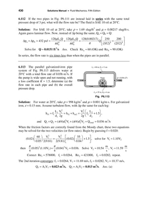


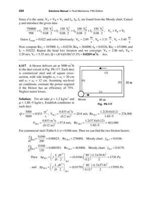
![Chapter 6 • Viscous Flow in Ducts 435
The total power required, at 75% efficiency, is thus:
Q∆p (0.833 m3 /s)(1730 + 17050 Pa)
Power = = = 20900 W Ans.
η 0.75
6.118 For the piping system of Fig. P6.118,
all pipes are concrete with a roughness
of 0.04 inch. Neglecting minor losses,
compute the overall pressure drop p1 − p2
in lbf/in2. The flow rate is 20 ft3/s of water
at 20°C.
Solution: For water at 20°C, take ρ =
1.94 slug/ft3 and µ = 2.09E−5 slug/ft⋅s. Fig. P6.118
Since the pipes are all different make a
little table of their respective L/d and ε/d:
(a) L = 1000 ft, d = 12 in, L/d = 1000, ε/d = 0.00333
(b) 1500 ft 8 in 2250 0.00500
(c) 800 ft 12 in 800 0.00333
(d) 1200 ft 15 in 960 0.00267
With the flow rate known, we can find everything in pipe (a):
Qa 20 ft 1.94(25.5)(1)
Va = = = 25.5 , Rea = = 2.36E6, fa ≈ 0.0270
Aa (π /4)(1 ft)2 s 2.09E−5
Then pipes (b,c,d) are in parallel, each having the same head loss and with flow rates
which must add up to the total of 20 ft3/s:
8fb L b Q 2 8f L Q 2 8f L Q 2 ft 3
h fb = b
= h fc = c2 c 5c = h fd = d2 d 5 d , and Q b + Q c + Q d = 20
π 2g d5 b π g dc π g dd s
Introduce Lb, db, etc. to find that Qc = 3.77Qb(fb/fc)1/2 and Qd = 5.38Qb(fb/fd)1/2
Then the flow rates are iterated from the relation
ft 3
å Q = 20 = Q b [1 + 3.77(fb /fc )1/2 + 5.38(fb /fd )1/2 ]
s
First guess: fb = fc = fd : Q b ≈ 1.97 ft 3 /s; Q c ≈ 7.43 ft 3 /s; Q d ≈ 10.6 ft 3 /s](https://image.slidesharecdn.com/solucionariodefluidoswhite-120604143132-phpapp02/85/Solucionario-de-fluidos_white-435-320.jpg)
![436 Solutions Manual • Fluid Mechanics, Fifth Edition
Improve by computing Reb ≈ 349000, fb ≈ 0.0306, Rec ≈ 878000, fc ≈ 0.0271, Red ≈
1002000, fd ≈ 0.0255. Repeat to find Qb ≈ 1.835 ft3/s, Qc ≈ 7.351 ft3/s, Qd ≈ 10.814 ft3/s.
Repeat once more and quit: Qb ≈ 1.833 ft3/s, Qc ≈ 7.349 ft3/s, Qd ≈ 10.819 ft3/s, from
which Vb ≈ 5.25 ft/s, Vc ≈ 9.36 ft/s, Vd ≈ 8.82 ft/s. The pressure drop is
La ρ Va2 L b ρ Vb
2
p1 − p 2 = ∆pa + ∆p b = fa + fb
da 2 db 2
lbf
= 17000 + 1800 ≈ 18800 psf ≈ 131 Ans.
in 2
6.119 Modify Prob. 6.118 as follows. Let the pressure drop (p1 − p2) be 98 lbf/in2.
Neglecting minor losses, determine the flow rate in ft3/s.
Solution: From the solution just above for ∆p ≈ 131 psi, we can see that ∆pa is about
90.2% of the total drop. Therefore our first guess can be that
L a ρVa2 1.94Va2
∆pa ≈ 0.902 ∆p = 0.902(98 × 144) ≈ 12729 psf = fa ≈ (0.027)(1000)
da 2 2
ft
Solve for Va ≈ 22.05
s
ft 3 ?
and Qa = Aa Va ≈ 17.3 = Q b [1 + 3.77(fb /fc )1/2 + 5.38(fb /fd )1/2 ]
s
The last relation is still valid just as it was in Prob. 6.188. We can iterate to find
ft 3 ft 3 ft 2
fa ≈ 0.0270, Q b ≈ 1.585 , Q c ≈ 6.357 , Q d ≈ 9.358 , fb ≈ 0.0307
s s s
p1 − p2 = fa (La /d a )(ρVa2 /2) + fb (L b /d b )(ρVb /2) ≈ 12717 + 1382 = 14099 psf ≈ 97.9 psi
2
This is certainly close enough. We conclude the flow rate is Q ≈ 17.3 ft3/s. Ans.
6.120 Three cast-iron pipes are laid in parallel with these dimensions:
Pipe 1: L1 = 800 m d1 = 12 cm
Pipe 2: L2 = 600 m d2 = 8 cm
Pipe 3: L3 = 900 m d3 = 10 cm
The total flow rate is 200 m3/h of water at 20°C. Determine (a) the flow rate in each pipe;
and (b) the pressure drop across the system.](https://image.slidesharecdn.com/solucionariodefluidoswhite-120604143132-phpapp02/85/Solucionario-de-fluidos_white-436-320.jpg)
![Chapter 6 • Viscous Flow in Ducts 437
Solution: For water at 20°C, take ρ = 998 kg/m3 and µ = 0.001 kg/m⋅s. For cast iron, ε =
0.26 mm. Then, ε/d1 = 0.00217, ε/d2 = 0.00325, and ε/d3 = 0.0026. The head losses are
the same for each pipe, and the flow rates add:
2 2 2
8 f1L1Q1 8 f2 L2Q2 8 f3 L3Q3 200 m3
hf = = 2 5 = 2 5 ; and Q1 + Q2 + Q3 =
π 2 gd1
5
π gd2 π gd3 3600 s
Substitute and combine: Q1[1 + 0.418( f1 / f2 )1/2 + 0.599( f1 / f3 )1/2 ] = 0.0556 m3 /s
We could either go directly to EES or begin by guessing f1 = f2 = f3, which gives Q1 =
0.0275 m3/s, Q2 = 0.0115 m3/s, and Q3 = 0.0165 m3/s. This is very close! Further iteration
gives
Re1 = 298000, f1 = 0.0245; Re 2 = 177000, f2 = 0.0275; Re3 = 208000, f3 = 0.0259
Q1 = 0.0281 m 3 /s, Q2 = 0.0111 m 3 /s, and Q3 = 0.0163 m 3 /s Ans. (a)
hf = 51.4 m, ∆p = ρ ghf = (998 kg/m 3 )(9.81 m/s2 )(51.4 m) = 503, 000 Pa Ans. (b)
6.121 Consider the three-reservoir system
of Fig. P6.121 with the following data:
L1 = 95 m L2 = 125 m L3 = 160 m
z1 = 25 m z2 = 115 m z3 = 85 m
All pipes are 28-cm-diameter unfinished
concrete (ε = 1 mm). Compute the steady
flow rate in all pipes for water at 20°C. Fig. P6.121
Solution: For water at 20°C, take ρ = 998 kg/m3 and µ = 0.001 kg/m⋅s. All pipes have
ε/d = 1/280 = 0.00357. Let the intersection be “a.” The head loss at “a” is desired:
L1 V12 L V2 L V2
z1 − h a = f1 ; z 2 − h a = f2 2 2 ; z3 − h a = f3 3 3
d1 2g d 2 2g d3 2g
plus the requirement that Q1 + Q2 + Q3 = 0 or, for same d, V1 + V2 + V3 = 0
We guess ha then iterate each friction factor to find V and Q and then check if åQ = 0.
2
æ 95 ö V1 m
ha = 75 m: 25 − 75 = (−)50 = f1 ç ÷ , solve f1 ≈ 0.02754, V1 ≈ −10.25
è 0.28 ø 2(9.81) s](https://image.slidesharecdn.com/solucionariodefluidoswhite-120604143132-phpapp02/85/Solucionario-de-fluidos_white-437-320.jpg)

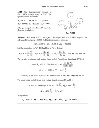
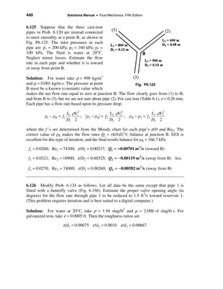


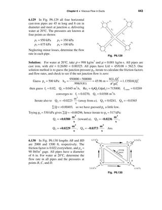
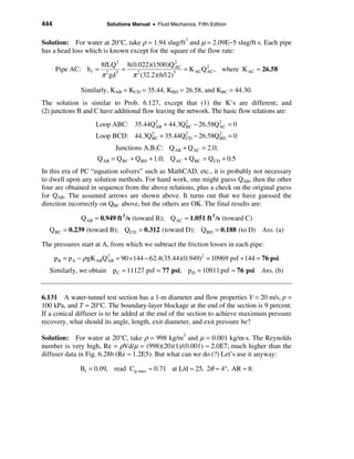
![Chapter 6 • Viscous Flow in Ducts 445
Then θ cone ≈ 2°, L ≈ 25d ≈ 25 m, Dexit = d(8)1/2 ≈ 2.8 m Ans. (a)
pe − p t p − 100000
Cp ≈ 0.71 = = e , or: pexit ≈ 242000 Pa Ans. (b)
(1/2)ρ Vt 2
(1/2)(998)(20)2
6.132 For Prob. 6.131, suppose we are limited by space to a total diffuser length of
10 meters. What should be the diffuser angle, exit diameter, and exit pressure for
maximum recovery?
Solution: We are limited to L/D = 10.0. From Fig. 6.28b, read Cp,max ≈ 0.62 at AR ≈ 4
and 2θ ≈ 6°. Ans. The exit diameter and pressure are
De = d √(AR) = (1.0)(4.0)1/2 ≈ 2.0 m Ans.
Cp,max ≈ 0.62 = (p e − 100000)/[(1/2)(998)(20)2 ], or: p exit ≈ 224000 Pa Ans.
6.133 A wind-tunnel test section is 3 ft square with flow properties V = 150 ft/s, p = 15 lbf/in2
absolute, and T = 68°F. Boundary-layer blockage at the end of the test section is 8 percent.
Find the angle, length, exit height, and exit pressure of a flat-walled diffuser added onto
the section to achieve maximum pressure recovery.
Solution: For air at 20°C and 15 psi, take ρ = 0.00238 slug/ft3 and µ = 3.76E−7 slug/ft⋅s.
The Reynolds number is rather high, Re = ρVd/µ = (0.00238)(150)(3)/(3.76E−7) ≈ 2.9E6;
much higher than the diffuser data in Fig. 6.28a (Re ≈ 2.8E5). But what can we do (?)
Let’s use it anyway:
Bt = 0.08, read Cp,max ≈ 0.70 at L/W1 ≈ 17, 2θ ≈ 9.5°, AR ≈ 3.75:
Then θ best ≈ 4.75° , L ≈ 17W1 ≈ 51 ft, W2 ≈ (AR)W1 = 3.75(3) ≈ 11 ft Ans.
pe − p t p e − 15 × 144 lbf
Cp ≈ 0.70 = = , or: pexit ≈ 2180 2 Ans.
(1/2)ρV1 (1/2)(0.00238)(150)
2 2
ft
6.134 For Prob. 6.133 above, suppose we are limited by space to a total diffuser length
of 30 ft. What should the diffuser angle, exit height, and exit pressure be for maximum
recovery?](https://image.slidesharecdn.com/solucionariodefluidoswhite-120604143132-phpapp02/85/Solucionario-de-fluidos_white-445-320.jpg)
![446 Solutions Manual • Fluid Mechanics, Fifth Edition
Solution: We are limited to L/W1 = 10.0. From Fig. 6.28a, read Cp,max ≈ 0.645 at AR ≈
2.8 and 2θ ≈ 10°. Ans. The exit height and pressure are
Wl,e = (AR)W1 = (2.8)(3.0) ≈ 8.4 ft Ans.
lbf
Cp,max ≈ 0.645 = [p e − (15)144)]/[(1/2)(0.00238)(150)2 ], or p e = 2180 Ans.
ft 2
6.135 An airplane uses a pitot-static tube as a velocimeter. The measurements, with
their uncertainties, are a static temperature of (−11 ± 3)°C, a static pressure of 60 ± 2 kPa,
and a pressure difference (po − ps) = 3200 ± 60 Pa. (a) Estimate the airplane’s velocity and
its uncertainty. (b) Is a compressibility correction needed?
Solution: The air density is ρ = p/(RT) = (60000 Pa)/[(287 m2/s2⋅K)(262 K)] = 0.798 kg/m3.
(a) Estimate the velocity from the incompressible Pitot formula, Eq. (6.97):
2 ∆p 2 ∆p 2(3200 Pa) m
V= = = = 90
ρ p/( RT ) 0.798 kg/m 3 s
The overall uncertainty involves pressure difference, absolute pressure, and absolute
temperature:
1/2 1/2
δ V éæ 1 δ∆p ö æ 1 δ p ö æ 1 δ T ö ù 1 éæ 60 ö æ 2 ö æ 3 ö ù
2 2 2 2 2 2
= êç ÷ +ç ÷ +ç ÷ ú = êç ÷ +ç ÷ +ç ÷ ú = 0.020
V êè 2 ∆p ø è 2 p ø è 2 T ø ú
ë û
2 êè 3200 ø è 60 ø è 262 ø ú
ë û
The uncertainty in velocity is 2%, therefore our final estimate is V ≈ 90 ± 2 m/s Ans. (a)
Check the Mach number. The speed of sound is a = (kRT)1/2 = [1.4(287)(262)]1/2 = 324 m/s.
Therefore
Ma = V/a = 90/324 = 0.28 < 0.3. No compressibility correction is needed. Ans. (b)
6.136 For the pitot-static pressure arrange-
ment of Fig. P6.136, the manometer fluid is
(colored) water at 20°C. Estimate (a) the
centerline velocity, (b) the pipe volume
flow, and (c) the (smooth) wall shear
stress.
Fig. P6.136](https://image.slidesharecdn.com/solucionariodefluidoswhite-120604143132-phpapp02/85/Solucionario-de-fluidos_white-446-320.jpg)
![Chapter 6 • Viscous Flow in Ducts 447
Solution: For air at 20°C and 1 atm, take ρ = 1.2 kg/m3 and µ = 1.8E−5 kg/m⋅s. For
water at 20°C, take ρ = 998 kg/m3 and µ = 0.001 kg/m⋅s. The manometer reads
po − p = ( ρ water − ρair )gh = (998 − 1.2)(9.81)(0.040) ≈ 391 Pa
Therefore VCL = [2∆p/ ρ ]1/2 = [2(391)/1.2]1/2 ≈ 25.5 m/s Ans. (a)
We can estimate the friction factor and then compute average velocity from Eq. (6.43):
m ρVd 1.2(21.7)(0.08)
Guess Vavg ≈ 0.85VCL ≈ 21.7 , then Re d = = ≈ 115,700
s µ 1.8E−5
25.5 m
Then fsmooth ≈ 0.0175, Vbetter = ≈ 21.69 (converged)
[1 + 1.33 √ 0.0175] s
Thus the volume flow is Q = (π /4)(0.08)2 (21.69) ≈ 0.109 m 3 /s. Ans. (b)
f 0.0175
Finally, τ w = ρV 2 = (1.2)(21.69)2 ≈ 1.23 Pa Ans. (c)
8 8
6.137 For the 20°C water flow of
Fig. P6.137, use the pitot-static arrange-
ment to estimate (a) the centerline velocity
and (b) the volume flow in the 5-in-
diameter smooth pipe. (c) What error in
flow rate is caused by neglecting the 1-ft
elevation difference?
Solution: For water at 20°C, take ρ =
1.94 slug/ft3 and µ = 2.09E−5 slug/ft⋅s. For
the manometer reading h = 2 inches,
poB − pA = (SG merc − 1)(ρg)water h Fig. P6.137
+ ρwater g(1 ft) but from the energy equation,
p A − p B = ρwater gh f-AB − ρwater g(1 ft) Therefore p oB − p B = (SG − 1)ρgh mano + ρgh f-AB
where friction loss h f-AB ≈ f(∆L/d)(V 2 /2g)
Thus the pitot tube reading equals the manometer reading (of about 130 psf) plus the
friction loss between A and B (which is only about 3 psf), so there is only a small error:
1/2 1/2
é 2 ∆p ù é 2(130.6) ù
(SG − 1)ρgh = (13.56 − 1)(62.4)(2/12) ≈ 130.6 psf, VCL ≈ê ú =ê
ë ρ û ë 1.94 ú û](https://image.slidesharecdn.com/solucionariodefluidoswhite-120604143132-phpapp02/85/Solucionario-de-fluidos_white-447-320.jpg)
(0.16) ≈ 1294 Pa
L ρ V2 fL ρ V 2 ρ 2
Meanwhile, pA − p B = ρ gh f = f , or poB − pB = − 1294 = VCL
d 2 d 2 2
2
æ 10 ö æ 1.2 ö 2 1.2 æ V ö
Guess f ≈ 0.02, V ≈ 0.85VCL , whence 0.02 ç ÷ ç ÷ V − 1294 = ç ÷
è 0.06 ø è 2 ø 2 è 0.85 ø
m 1.2(33.3)(0.06)
Solve for V ≈ 33.3 , Re d = ≈ 133000, fbetter ≈ 0.0170,
s 1.8E−5
V ≈ VCL /[1 + 1.33 √ f] ≈ 0.852VCL , repeat to convergence
Finally converges, f ≈ 0.0164, V ≈ 39.87 m/s, VCL = V/0.8546 ≈ 46.65 m/s. Ans.](https://image.slidesharecdn.com/solucionariodefluidoswhite-120604143132-phpapp02/85/Solucionario-de-fluidos_white-448-320.jpg)
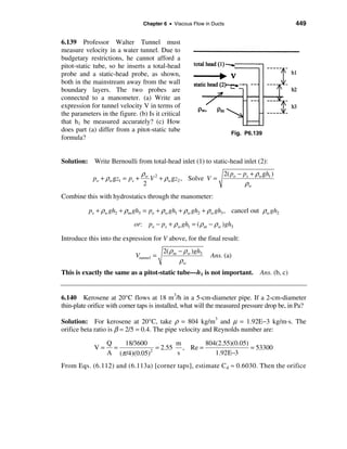
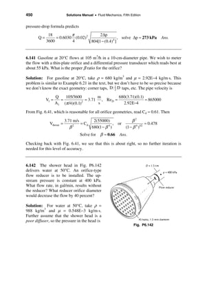
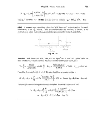

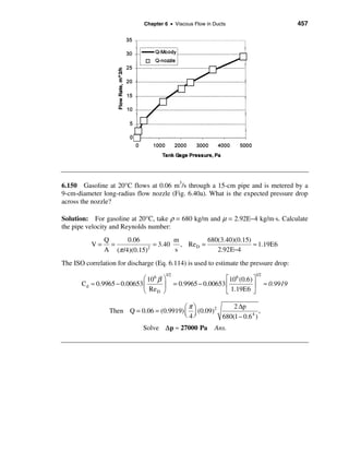

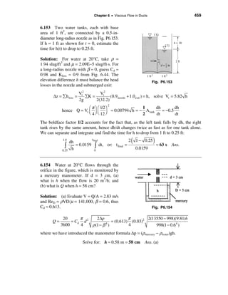

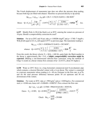


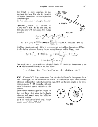
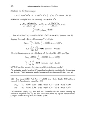

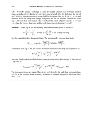


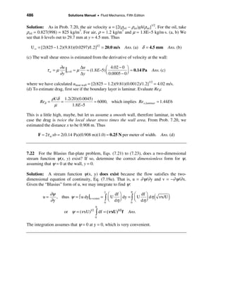
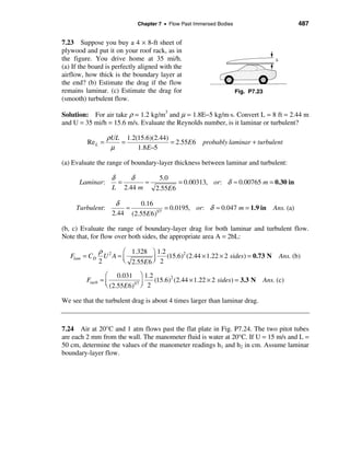


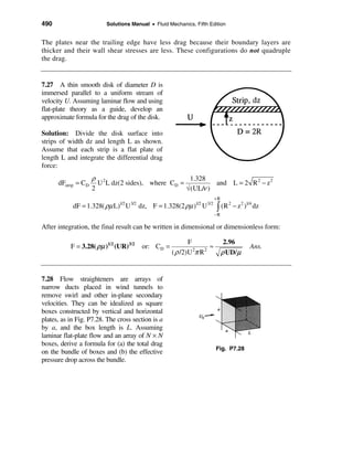
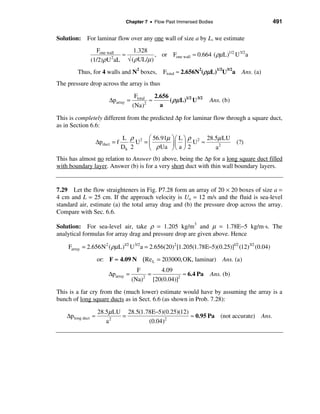
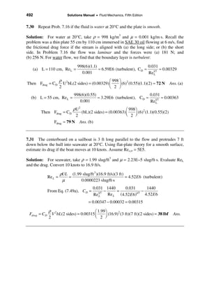


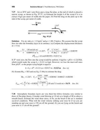


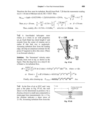


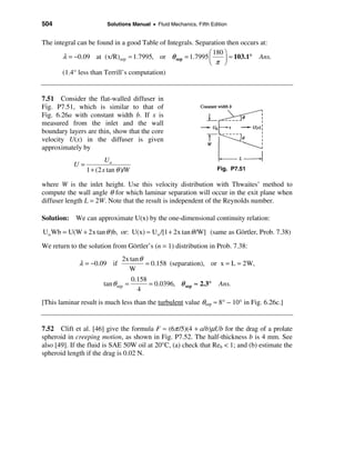
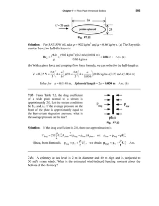


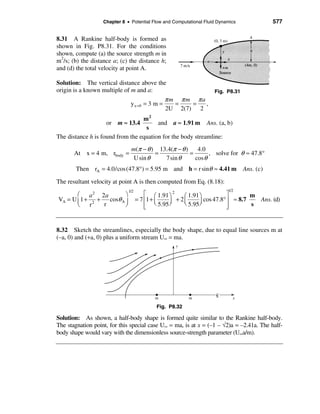


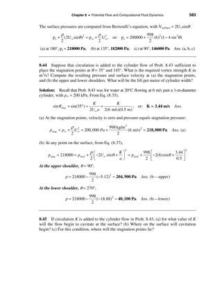

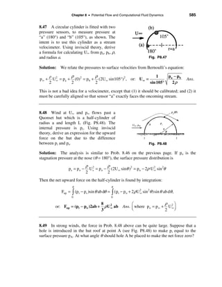
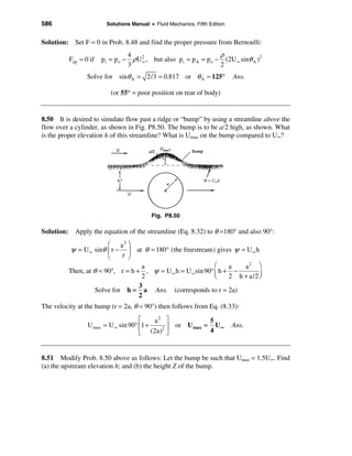


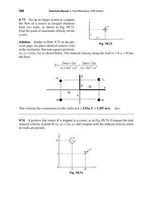


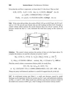


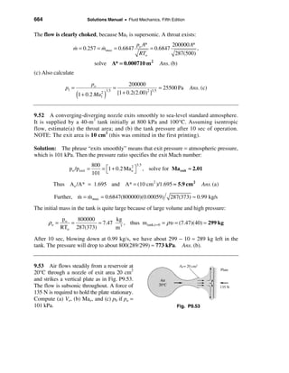


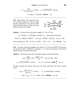
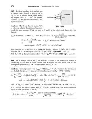


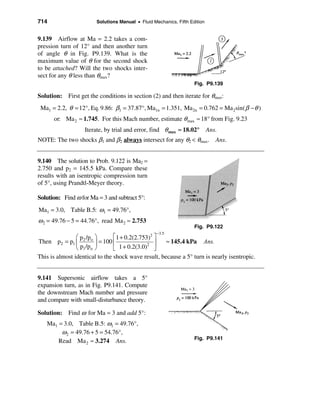

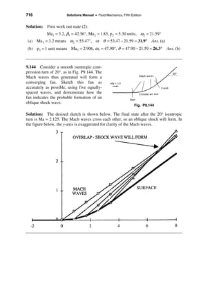


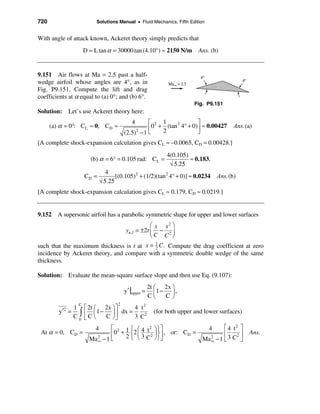
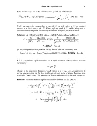


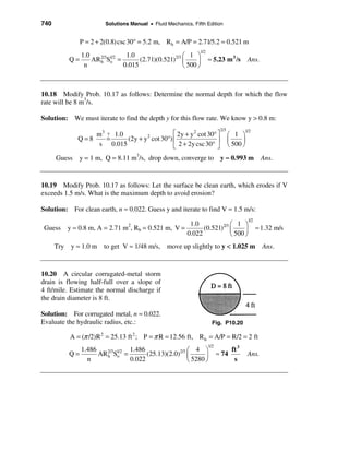


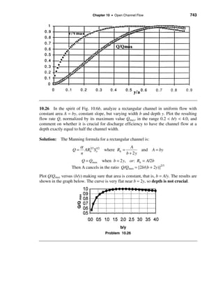


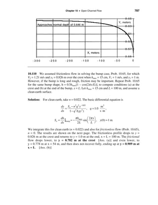
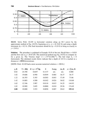
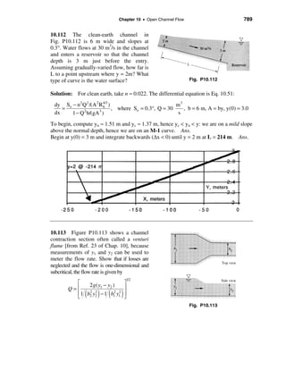
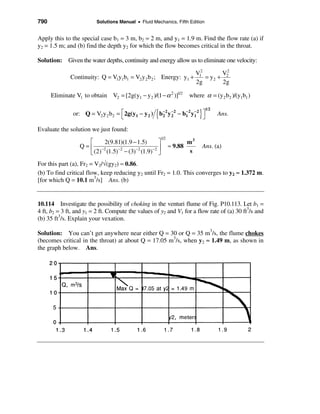


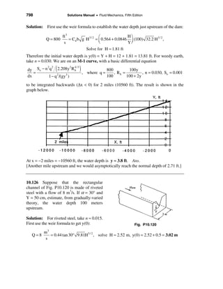

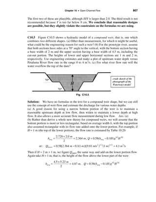

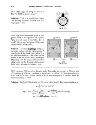
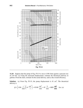


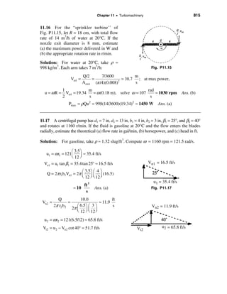

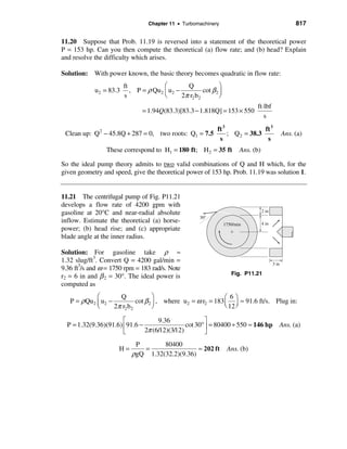
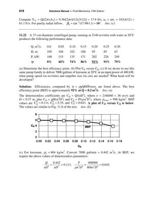


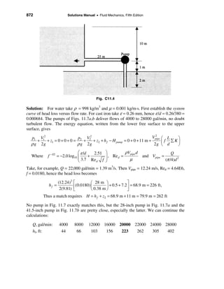


This document provides solutions to problems from Chapter 1 of an introductory fluid mechanics textbook. The key information is: 1) Problem 1.10 asks if the Stokes-Oseen formula for drag on a sphere is dimensionally homogeneous. The formula contains terms with dimensions of force, viscosity, diameter, velocity, density, and the student confirms it is homogeneous. 2) Problem 1.12 asks for the dimensions of the parameter B in an equation relating pressure drop, viscosity, radius, and velocity in laminar pipe flow. The student determines B has dimensions of inverse length. 3) Problem 1.13 calculates the efficiency of a pump given values for volume flow rate, pressure rise, and input power


![Mecanica de-fluidos-ejercicios[1]](https://cdn.slidesharecdn.com/ss_thumbnails/mecanica-de-fluidos-ejercicios1-160901222744-thumbnail.jpg?width=640&height=640&fit=bounds)


