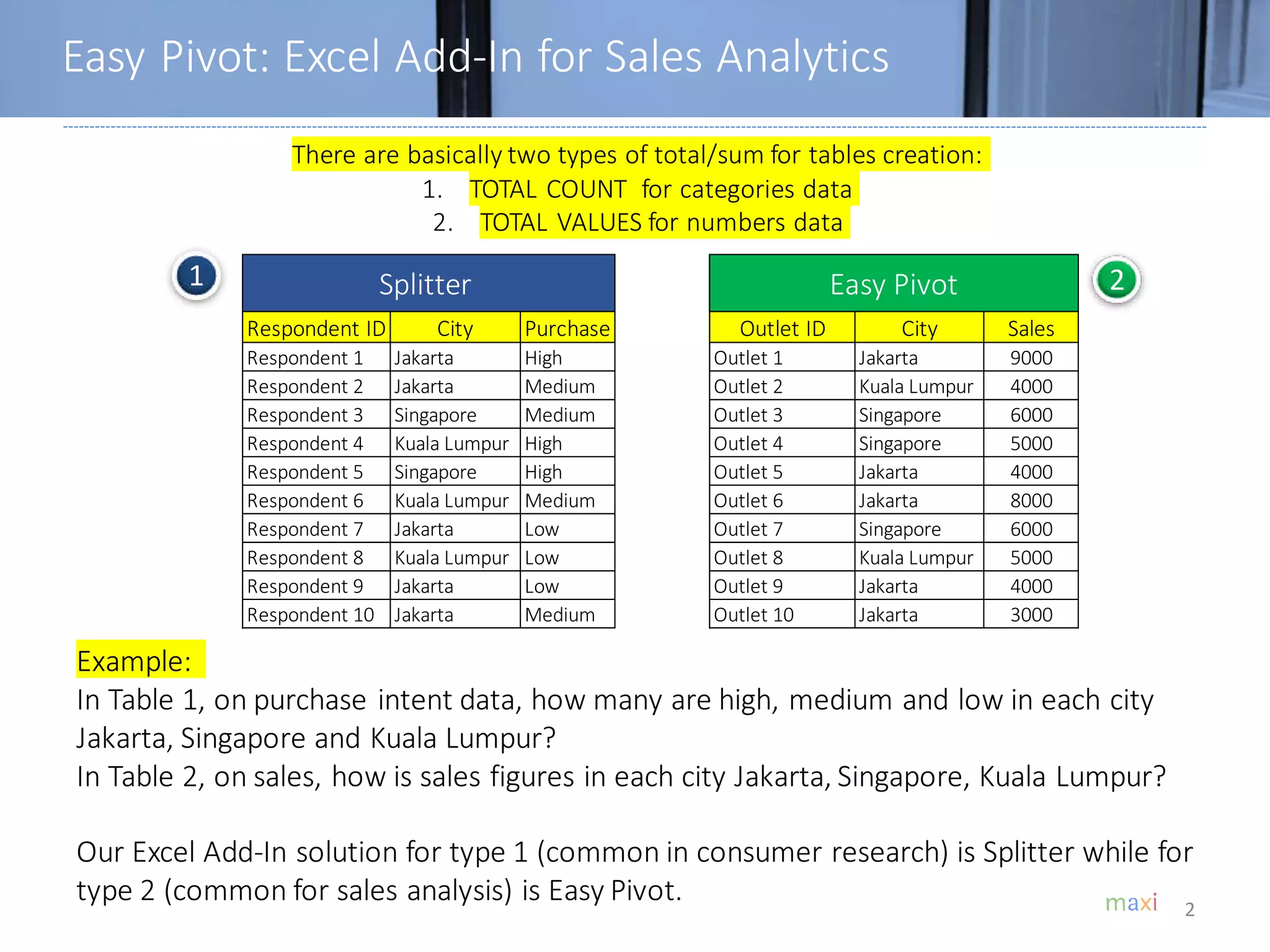
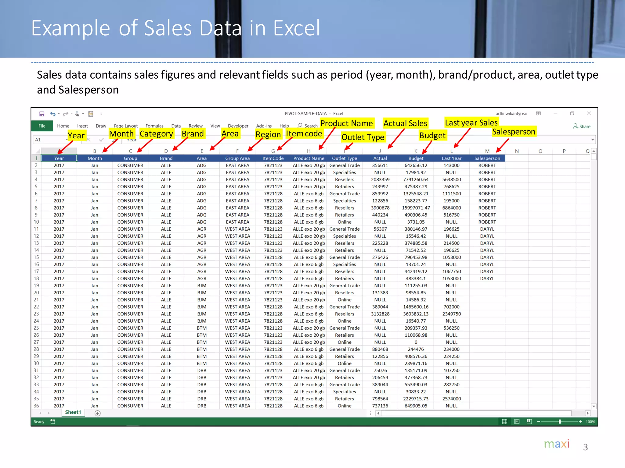
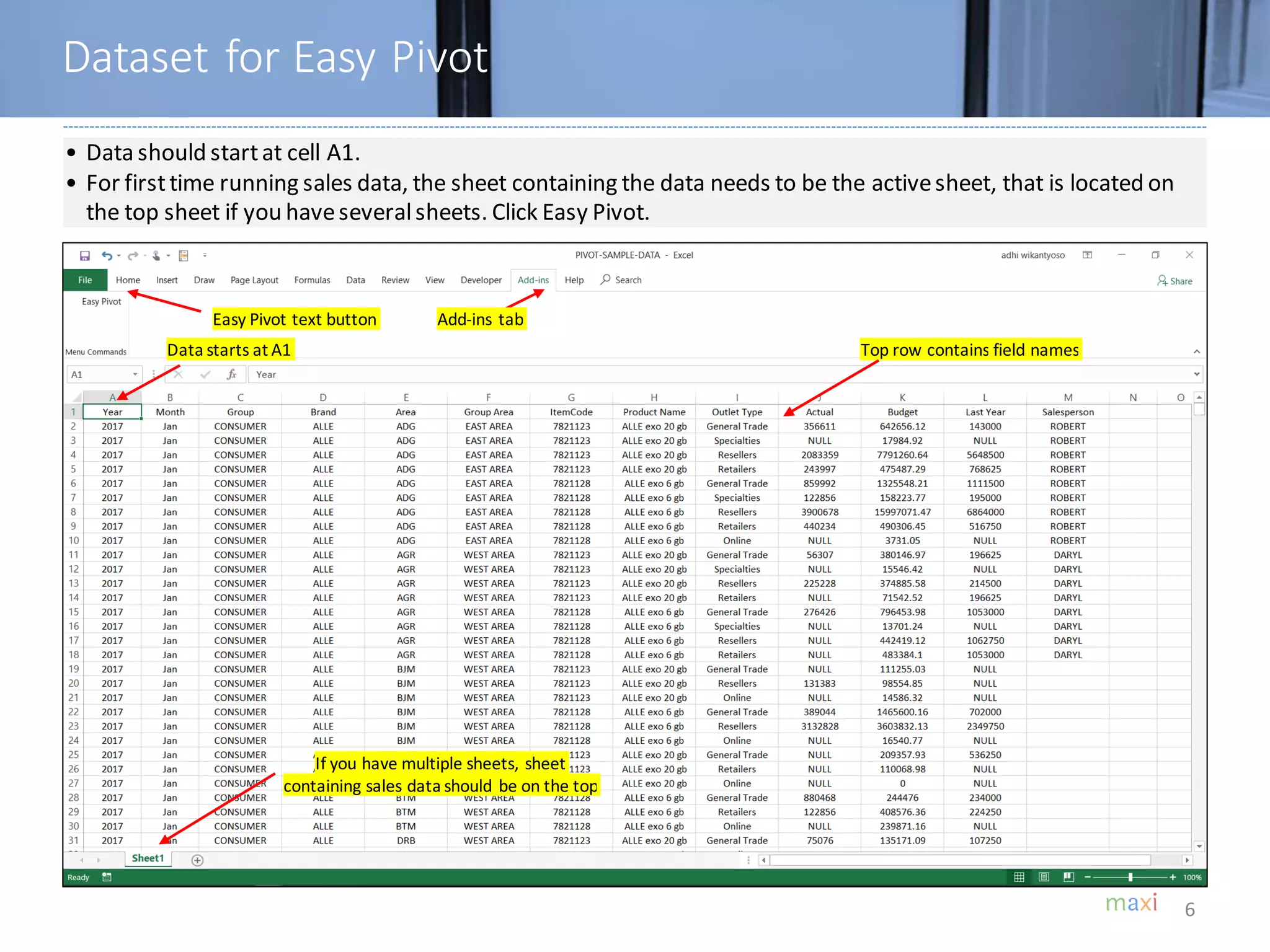
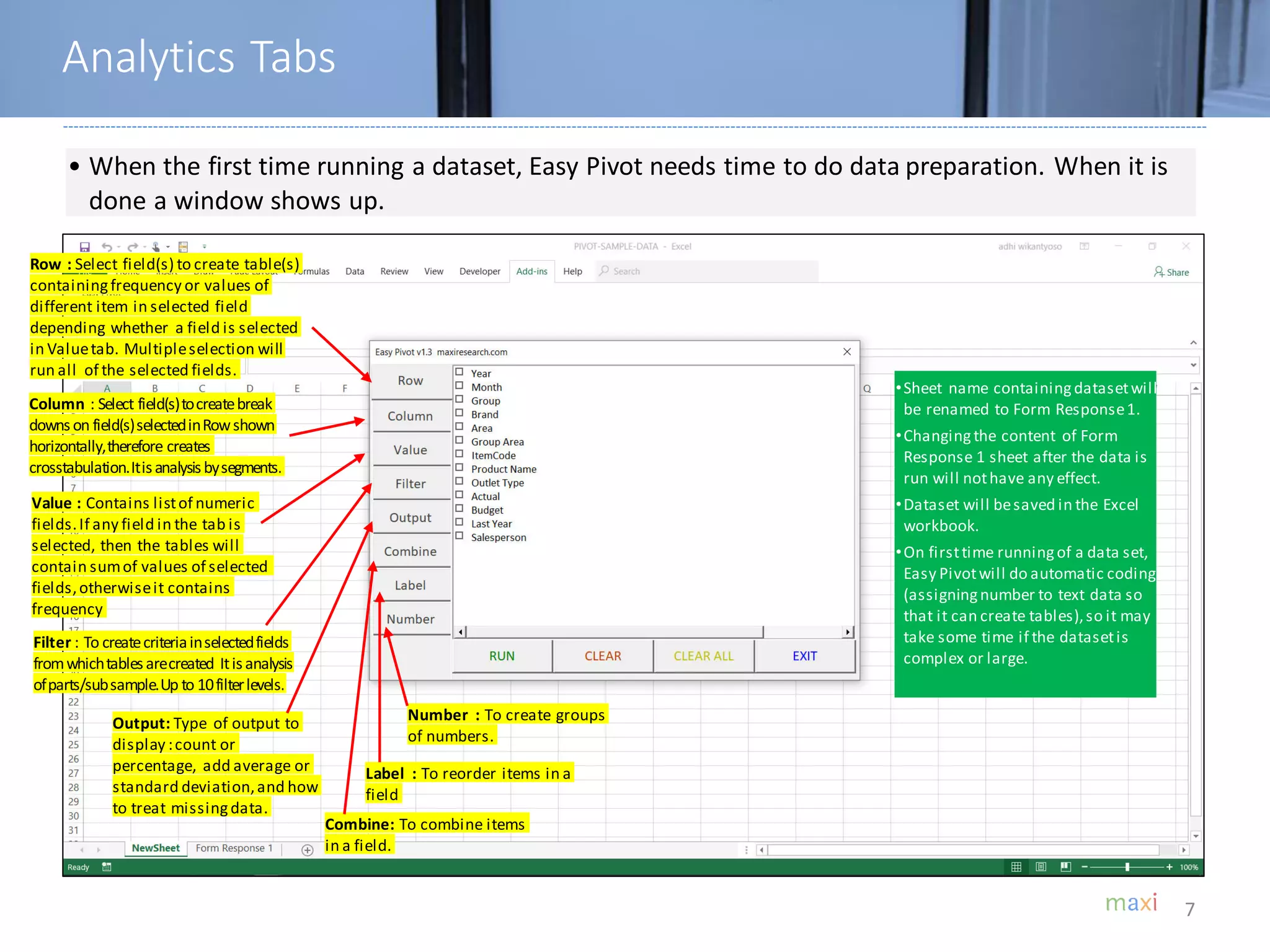
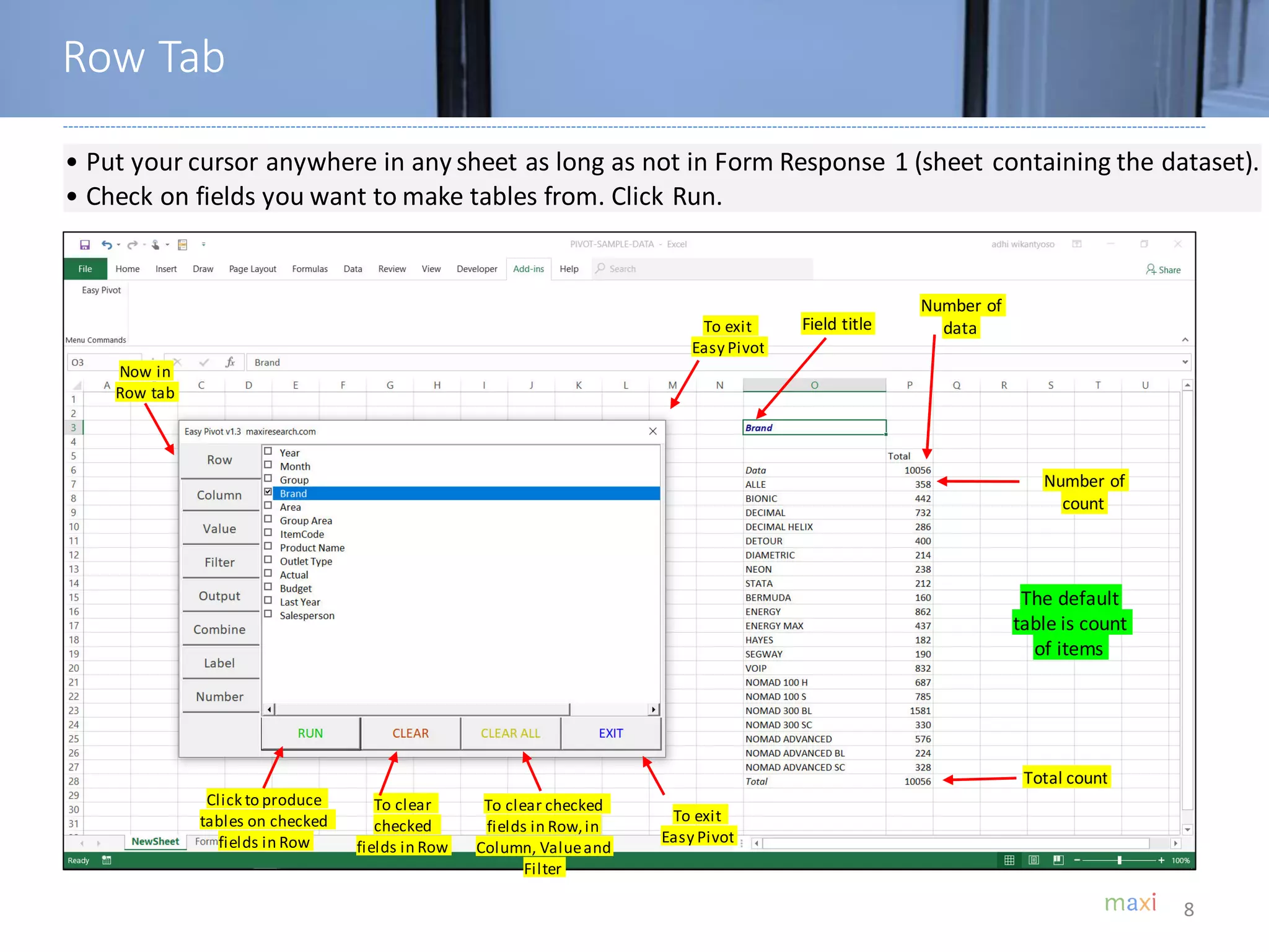
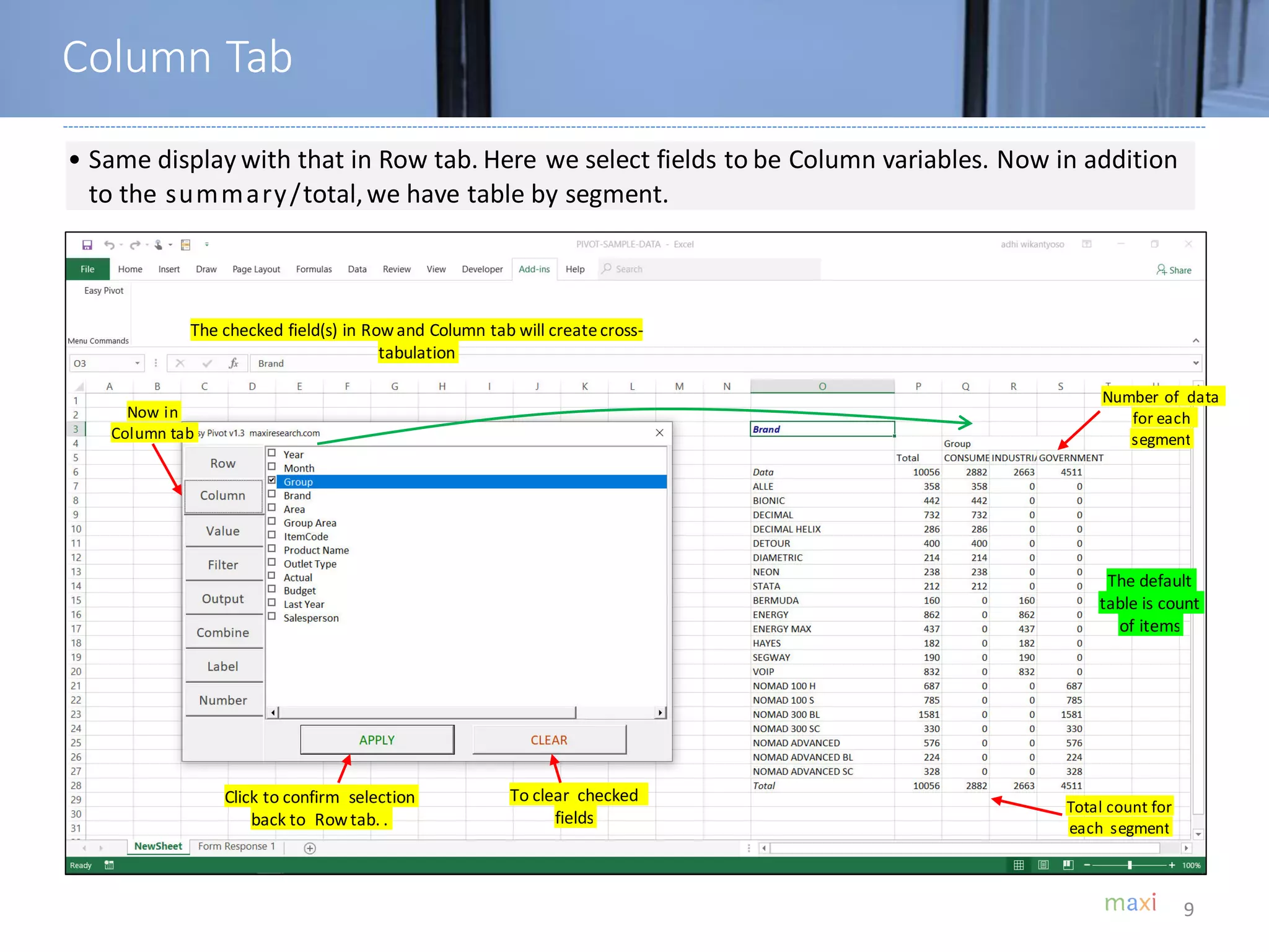
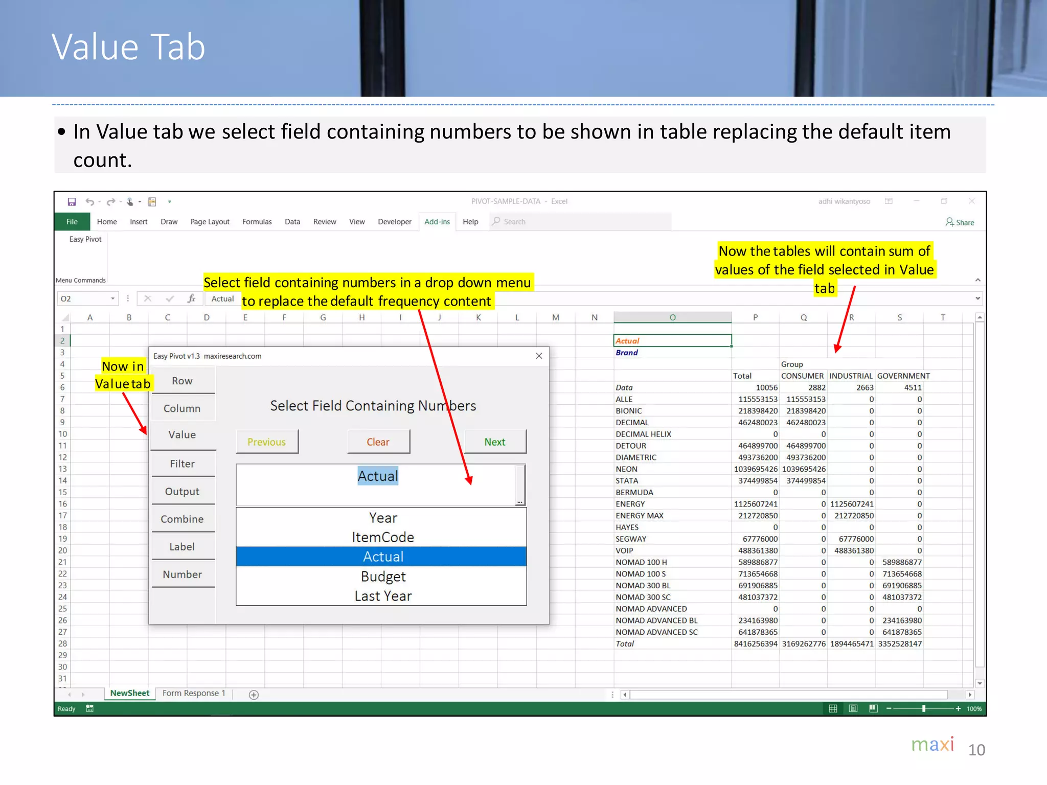
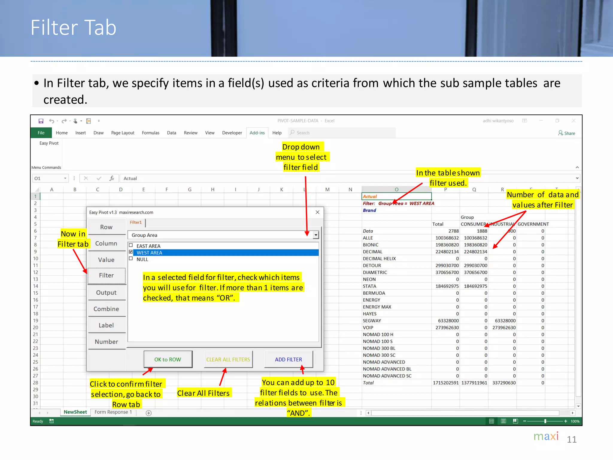
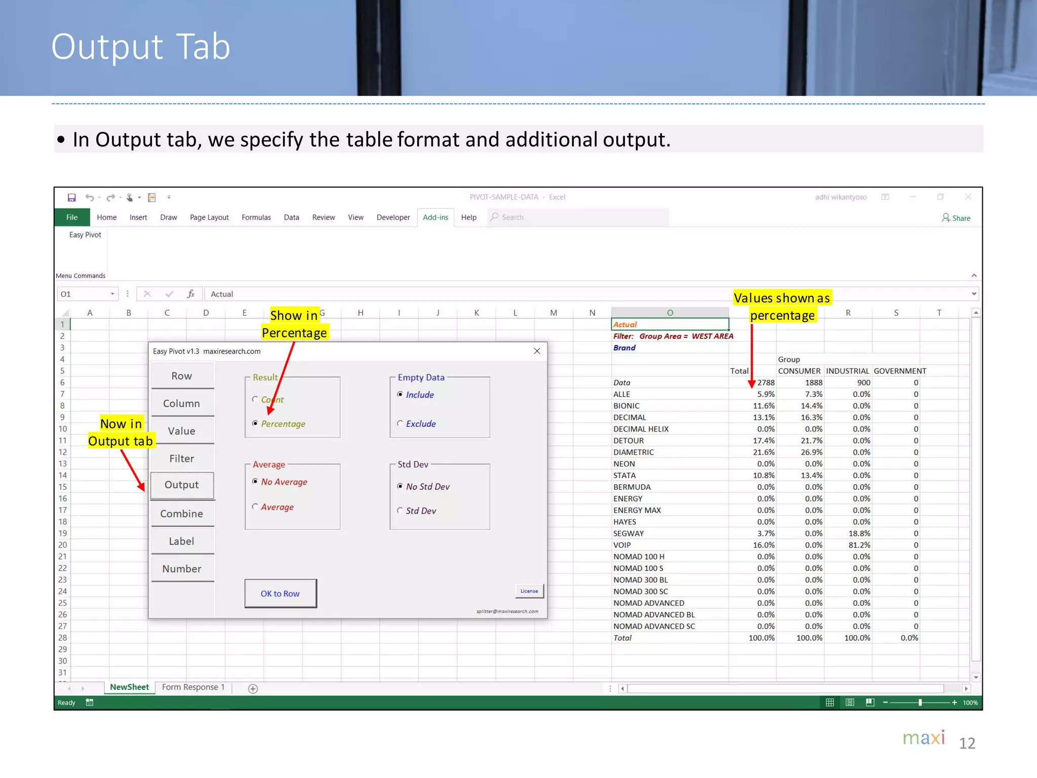
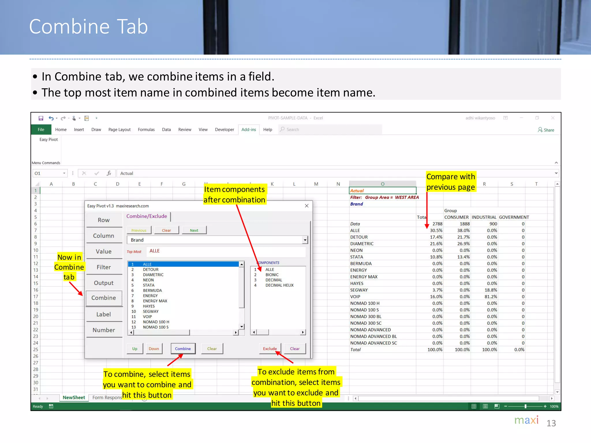
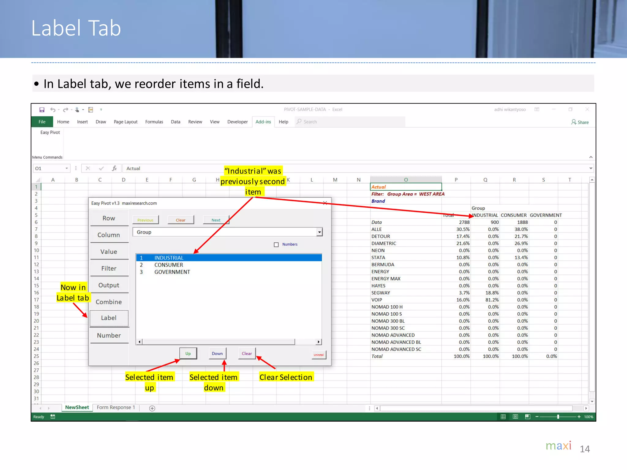
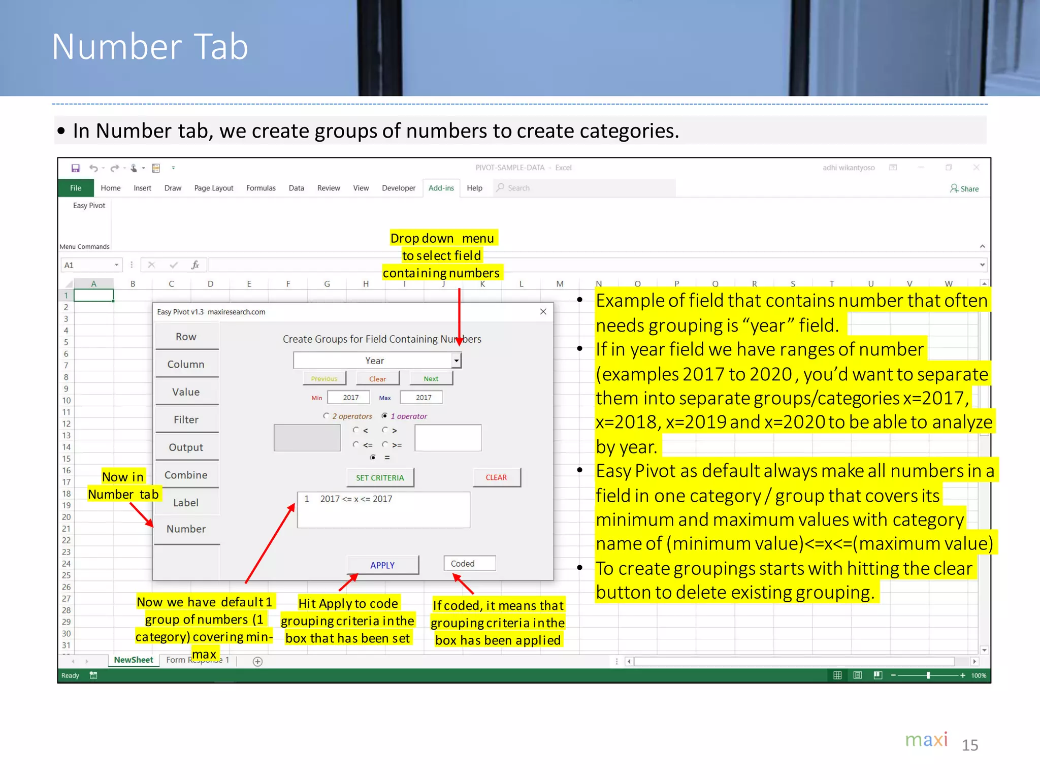
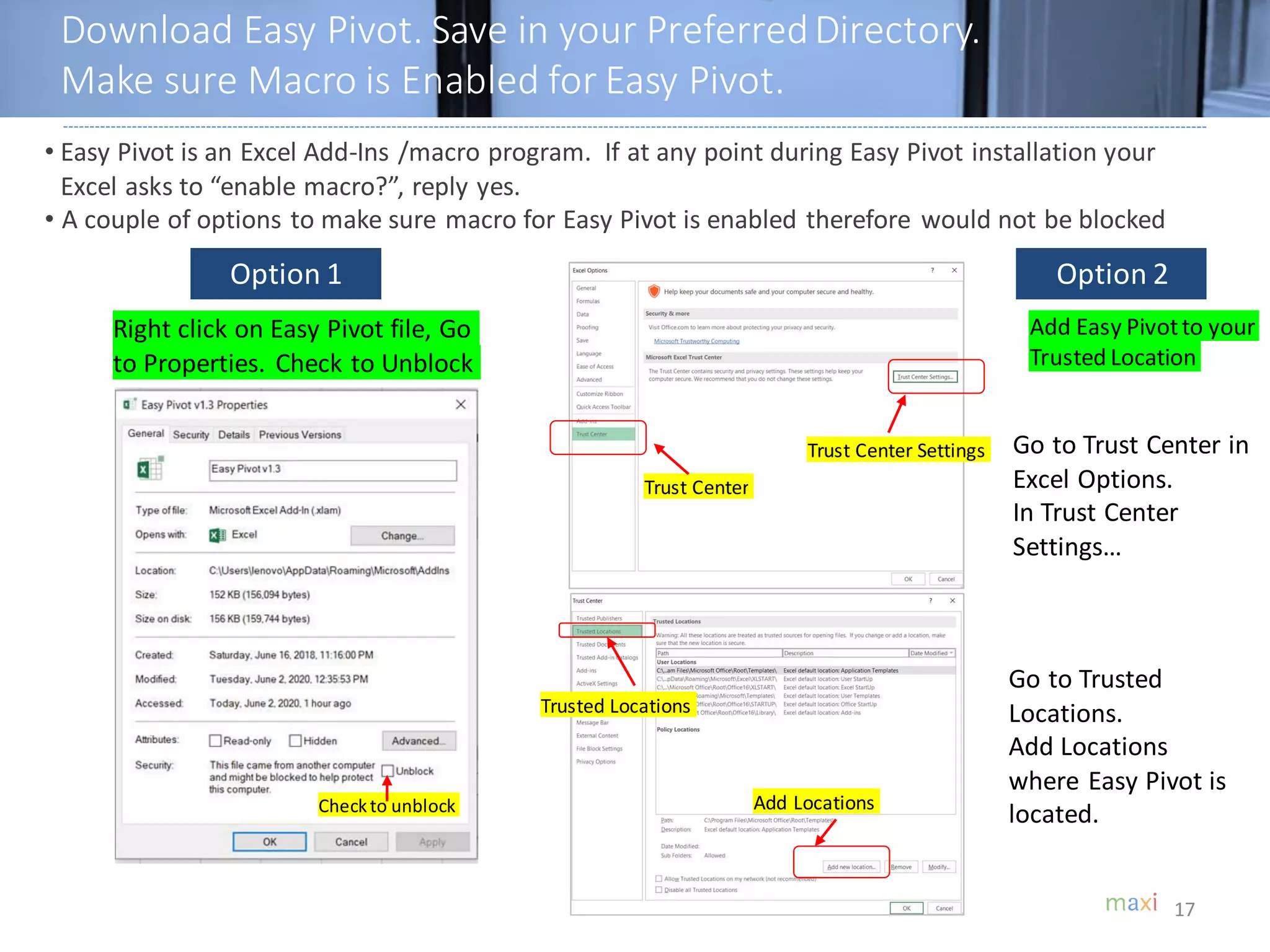
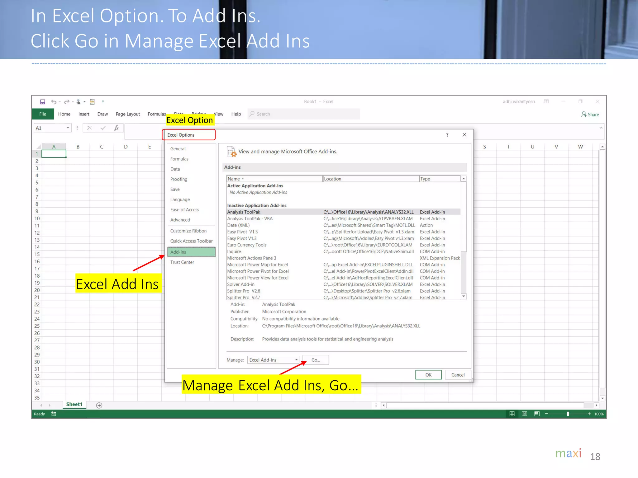
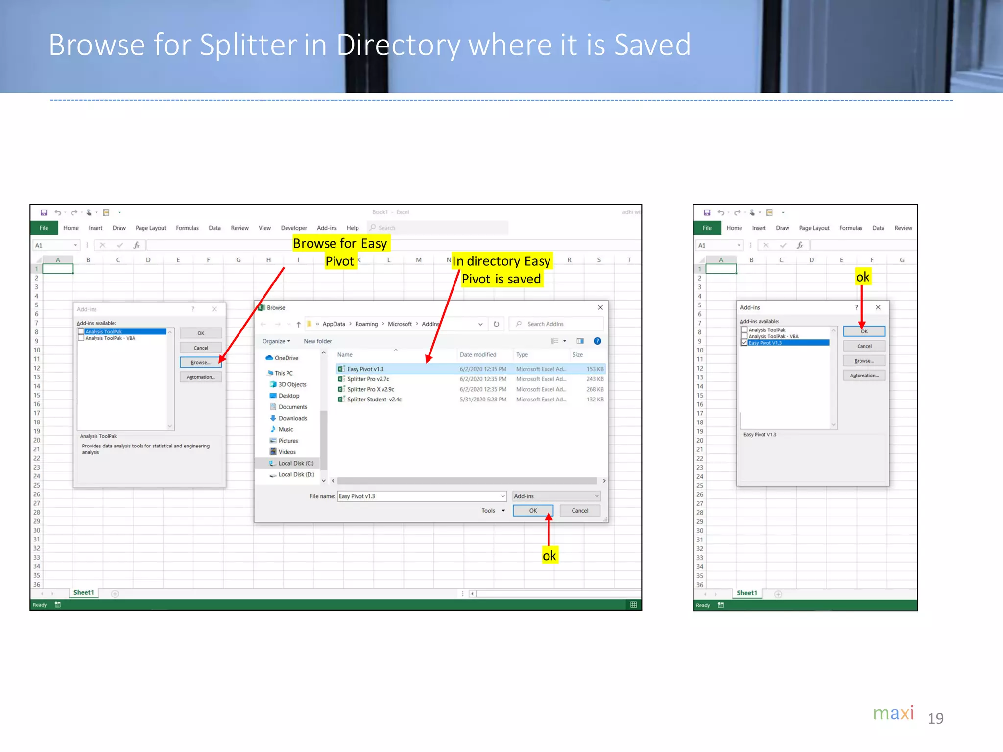
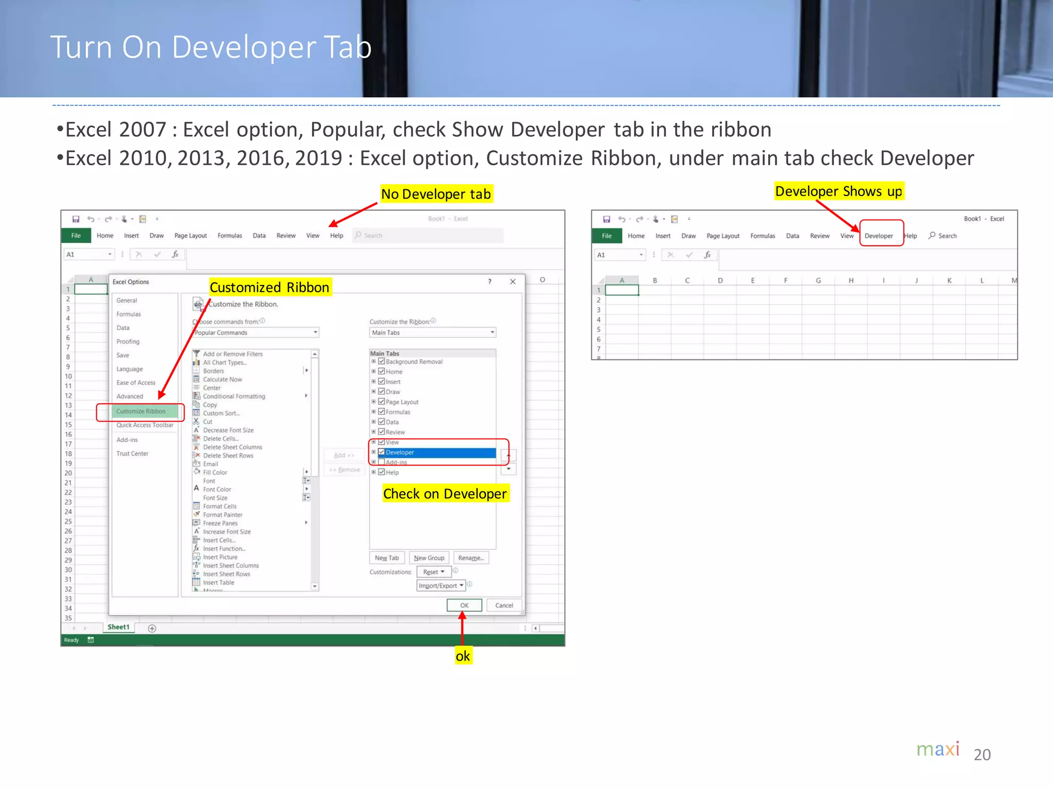
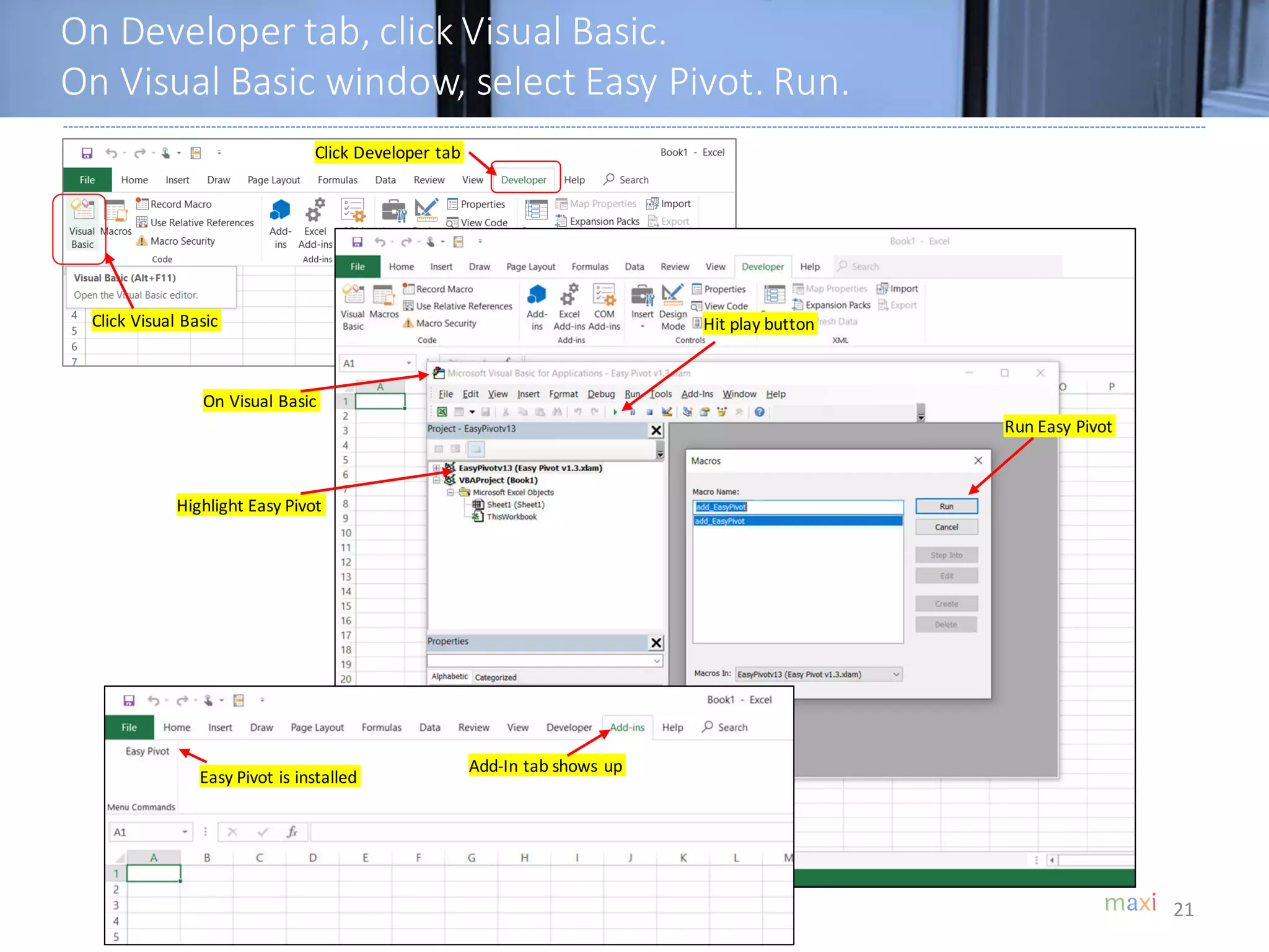
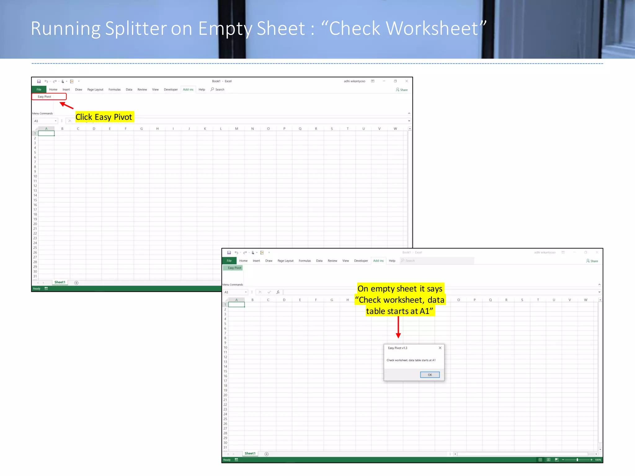
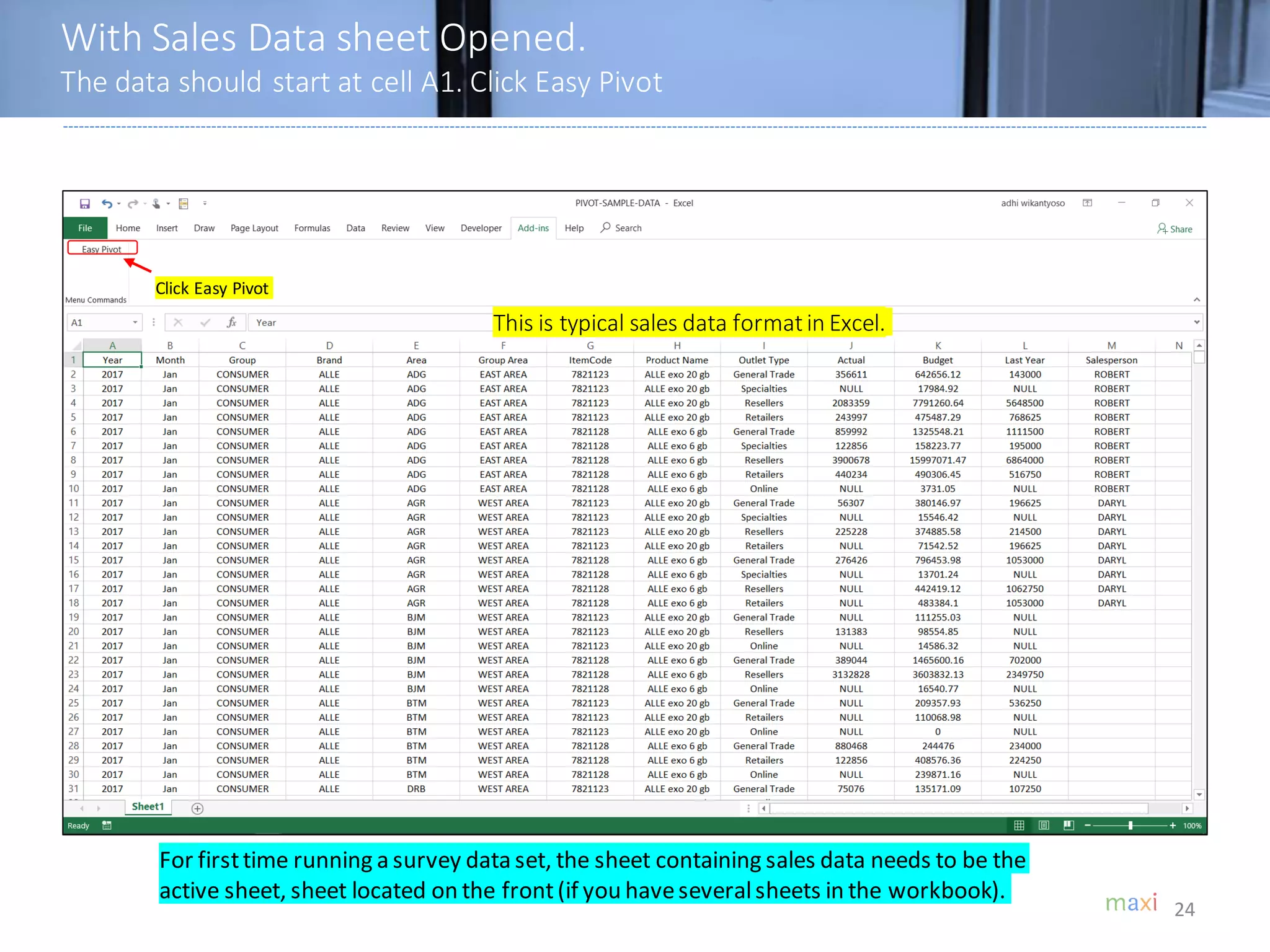
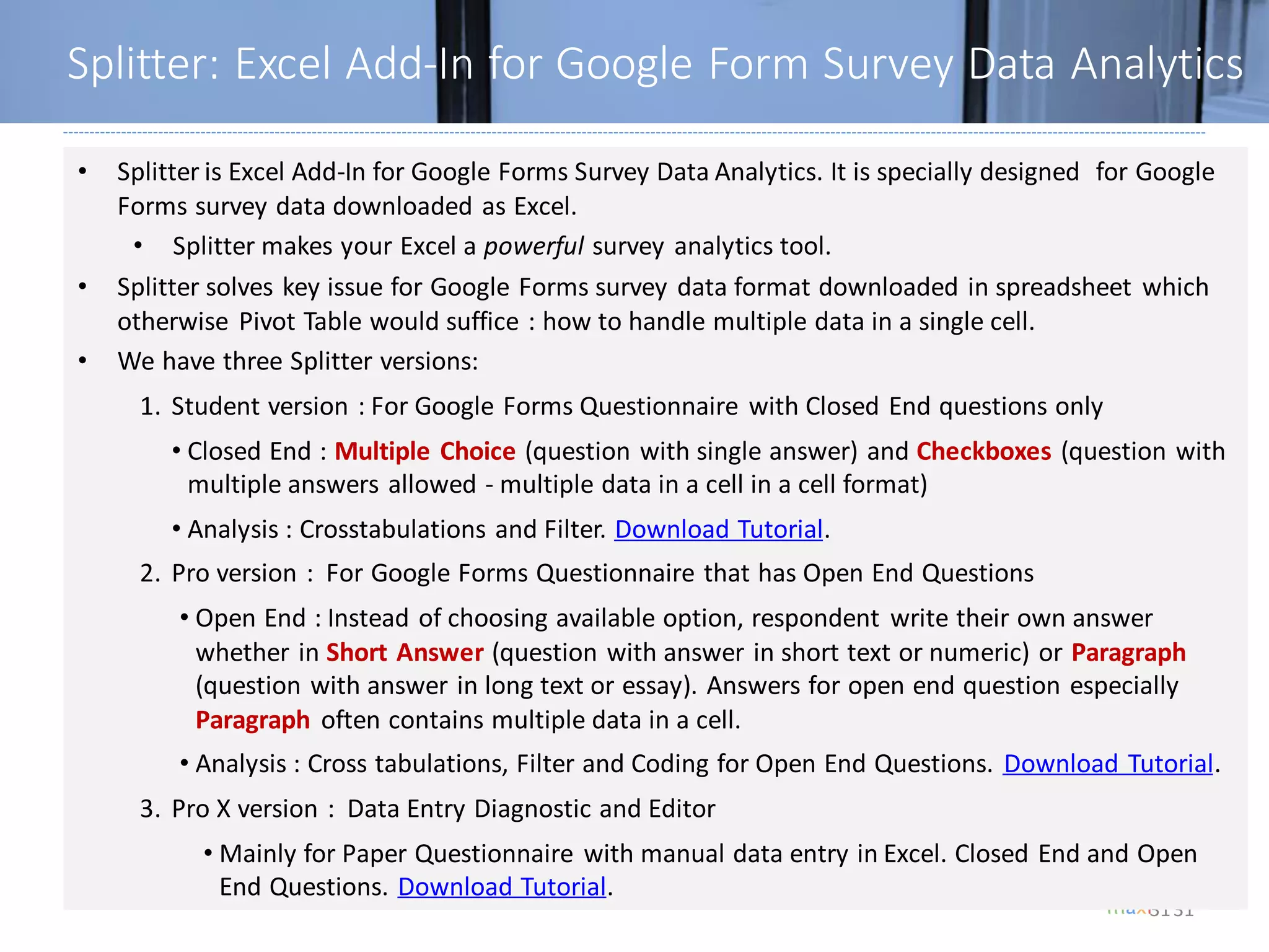
June 2020
Easy Pivot: Excel Add-In For Sales
Analytics Tutorial
Easy Pivot: Excel Add-In for Sales Analytics
2
There are basically two types of total/sum for tables creation:
1. TOTAL COUNT for categories data
2. TOTAL VALUES for numbers data
Example:
In Table 1, on purchase intent data, how many are high, medium and low in each city
Jakarta, Singapore and Kuala Lumpur?
In Table 2, on sales, how is sales figures in each city Jakarta, Singapore, Kuala Lumpur?
Our Excel Add-In solution for type 1 (common in consumer research) is Splitter while for
type 2 (common for sales analysis) is Easy Pivot.
1 2
Respondent ID City Purchase Outlet ID City Sales
Respondent 1 Jakarta High Outlet 1 Jakarta 9000
Respondent 2 Jakarta Medium Outlet 2 Kuala Lumpur 4000
Respondent 3 Singapore Medium Outlet 3 Singapore 6000
Respondent 4 Kuala Lumpur High Outlet 4 Singapore 5000
Respondent 5 Singapore High Outlet 5 Jakarta 4000
Respondent 6 Kuala Lumpur Medium Outlet 6 Jakarta 8000
Respondent 7 Jakarta Low Outlet 7 Singapore 6000
Respondent 8 Kuala Lumpur Low Outlet 8 Kuala Lumpur 5000
Respondent 9 Jakarta Low Outlet 9 Jakarta 4000
Respondent 10 Jakarta Medium Outlet 10 Jakarta 3000
Splitter Easy Pivot
Example of Sales Data in Excel
3
Sales data contains sales figures and relevantfields such as period (year, month), brand/product, area, outlettype
and Salesperson
Year Month Category Brand Area Region Itemcode
Product Name
Outlet Type
Actual Sales
Budget
Last year Sales
Salesperson
4
• DownloadEasyPivotfrom our GoogleDrive here
• How to Install and Run Easy Pivot in Appendixof this tutorial
• Downloadsample dataused in tutorial here (10k rows of data)
Download Links
5
EASY PIVOT
ANALYTICS
6
Top row contains field namesData starts at A1
• Data should startat cell A1.
• For firsttime running sales data, the sheet containing the data needs to be the activesheet, that is located on
the top sheet if you haveseveralsheets. Click Easy Pivot.
Easy Pivot text button
If you have multiple sheets, sheet
containing sales data should be on the top
Add-ins tab
Dataset for Easy Pivot
7
• When the first time running a dataset, Easy Pivot needs time to do data preparation. When it is
done a window shows up.
Row : Select field(s) to create table(s)
containingfrequency or values of
different item in selected field
depending whether a field is selected
in Valuetab. Multipleselection will
run all of the selected fields.
Column : Select field(s)tocreatebreak
downson field(s)selectedinRowshown
horizontally,therefore creates
crosstabulation.Itisanalysisbysegments.
Filter : To createcriteriainselectedfields
fromwhichtablesarecreated Itisanalysis
ofparts/subsample.Up to 10filterlevels.
Output: Type of output to
display :count or
percentage, add average or
standard deviation,and how
to treat missingdata.
•Sheet name containingdatasetwill
be renamed to Form Response1.
•Changingthe content of Form
Response 1 sheet after the data is
run will nothave any effect.
•Dataset will besaved in the Excel
workbook.
•On firsttime runningof a data set,
Easy Pivotwill do automatic coding
(assigningnumber to text data so
that it can create tables),so it may
take some time if the datasetis
complex or large.
Value : Contains listof numeric
fields.If any field in the tab is
selected, then the tables will
contain sumof values of selected
fields,otherwiseit contains
frequency
Combine: To combine items
in a field.
Label : To reorder items in a
field
Number : To create groups
of numbers.
Analytics Tabs
8
• Put your cursor anywhere in any sheet as long as not in Form Response 1 (sheet containing the dataset).
• Check on fields you want to make tables from. Click Run.
Click to produce
tables on checked
fields in Row
To clear
checked
fields in Row
To exit
Easy Pivot
To clear checked
fields in Row,in
Column, Valueand
Filter
To exit
Easy Pivot
Field title
Number of
data
Total count
Number of
count
The default
table is count
of items
Row Tab
Now in
Row tab
9
• Same display with that in Row tab. Here we select fields to be Column variables. Now in addition
to the summary/total,we have table by segment.
The checked field(s) in Rowand Column tab will createcross-
tabulation
Click to confirm selection
back to Rowtab. .
To clear checked
fields
Number of data
for each
segment
Total count for
each segment
The default
table is count
of items
Column Tab
Now in
Column tab
10
• In Value tab we select field containing numbers to be shown in table replacing the default item
count.
Select field containing numbers in a drop down menu
to replace thedefault frequency content
Now thetables will contain sum of
values of the field selected in Value
tab
Now in
Valuetab
Value Tab
11
• In Filter tab, we specify items in a field(s) used as criteria from which the sub sample tables are
created.
In a selected field for filter,check which items
you will usefor filter.If more than 1 items are
checked, that means “OR”.
Drop down
menu to select
filter field
In the tableshown
filter used.
Number of data and
values after Filter
Click to confirmfilter
selection,go back to
Row tab
Clear All Filters
You can add up to 10
filter fields to use.The
relations between filter is
“AND”.
Filter Tab
Now in
Filter tab
12
• In Output tab, we specify the table format and additional output.
Output Tab
Now in
Output tab
Show in
Percentage
Values shown as
percentage
13
• In Combine tab, we combine items in a field.
• The top most item name in combined items become item name.
Itemcomponents
after combination
To combine, select items
you want to combine and
hit this button
To exclude items from
combination, select items
you want to exclude and
hit this button
Now in
Combine
tab
Compare with
previous page
Combine Tab
14
• In Label tab, we reorder items in a field.
Selected item
up
Selected item
down
Clear Selection
“Industrial”was
previously second
item
Label Tab
Now in
Label tab
15
• In Number tab, we create groups of numbers to create categories.
Number Tab
Now in
Number tab
• Exampleof field that containsnumber thatoften
needs grouping is“year” field.
• If in year field we have rangesof number
(examples2017 to 2020, you’d wantto separate
them into separategroups/categoriesx=2017,
x=2018, x=2019and x=2020to beableto analyze
by year.
• EasyPivot as defaultalwaysmakeall numbersin a
field in one category/ group thatcoversits
minimum and maximum valueswith category
nameof (minimum value)<=x<=(maximum value)
• To creategroupingsstartswith hitting theclear
button to delete existing grouping.
Drop down menu
to select field
containingnumbers
Now we have default1
group of numbers (1
category) coveringmin-
max
If coded, it means that
groupingcriteria inthe
box has been applied
Hit Apply to code
groupingcriteria inthe
box that has been set
16
HOW TO INSTALL
EASY PIVOT
Download Easy Pivot. Save in your PreferredDirectory.
Make sure Macro is Enabled for Easy Pivot.
17
• Easy Pivot is an Excel Add-Ins /macro program. If at any point during Easy Pivot installation your
Excel asks to “enable macro?”, reply yes.
• A couple of options to make sure macro for Easy Pivot is enabled therefore would not be blocked
Right click on Easy Pivot file, Go
to Properties. Check to Unblock
Checkto unblock
Go to Trust Center in
Excel Options.
In Trust Center
Settings…
Go to Trusted
Locations.
Add Locations
where Easy Pivot is
located.
Option 1 Option 2
Trust Center
Trust Center Settings
Trusted Locations
Add Locations
Add Easy Pivotto your
Trusted Location
In Excel Option. To Add Ins.
Click Go in Manage Excel Add Ins
18
Excel Add Ins
Manage Excel Add Ins, Go…
Excel Option
Browse for Splitter in Directory where it is Saved
19
Browse for Easy
Pivot In directory Easy
Pivot is saved
ok
ok
Turn On Developer Tab
20
•Excel 2007 : Excel option, Popular, check Show Developer tab in the ribbon
•Excel 2010, 2013, 2016, 2019 : Excel option, Customize Ribbon, under main tab check Developer
Customized Ribbon
No Developer tab
Check on Developer
ok
Developer Shows up
On Developer tab, click Visual Basic.
On Visual Basic window, select Easy Pivot. Run.
21
Click Developer tab
Click Visual Basic
On Visual Basic
Highlight Easy Pivot
Hit play button
Run Easy Pivot
Add-In tab shows up
Easy Pivot is installed
22
RUN EASY PIVOT
Running Splitter on Empty Sheet : “Check Worksheet”
23
Click Easy Pivot
On empty sheet it says
“Check worksheet, data
table starts at A1”
With Sales Data sheet Opened.
The data should start at cell A1. Click Easy Pivot
24
This is typical sales data formatin Excel.
Click Easy Pivot
For firsttime running a survey data set, the sheet containing sales data needs to be the
active sheet, sheet located on the front(if you haveseveralsheets in the workbook).
Pop Up Window 7 Day Trial Period
25
Trial Period for 7 Days
We arenow in “New Sheet”
The sheet that contains sales data is
renamed “Form Response 1”
Click to Continue Trial
If you haven’tentered Activation Code
Enter Activation Code here
Clik to validate code
Easy Pivot Analytics Window Shows Up
26
Easy Pivot Analytics Window
Easy Pivot is Ready for Analysis
27
Now in Row tab
28
EASY PIVOT
ACTIVATION CODE
• After installingthere is a 7 day free trial
• Afterwards, Activation codecanbe purchasedonlinevia Paypal.
• Activationcodewill be sent to your Paypal emailright after payment.
• To ActivateEntercode in EasyPivot pop up window.
• This is not a subscription.After activation periodis over there is no automatic
renewal.
• You’d want to purchasecode to re-activateEasyPivot
29
Select ActivationPeriod Option
Will go to PayPal Landing Page
For alternative paymentmethod contactSplitter@maxiresearch.com
ActivationCode
1 Month
$2
3 Months
$5
6 Months
$8
1 Year
$12
30
OTHER EXCEL ADD IN
PRODUCTS
31
Splitter: Excel Add-In for Google Form Survey Data Analytics
31
• Splitter is Excel Add-In for Google Forms Survey Data Analytics. It is specially designed for Google
Forms survey data downloaded as Excel.
• Splitter makes your Excel a powerful survey analytics tool.
• Splitter solves key issue for Google Forms survey data format downloaded in spreadsheet which
otherwise Pivot Table would suffice : how to handle multiple data in a single cell.
• We have three Splitter versions:
1. Student version : For Google Forms Questionnaire with Closed End questions only
• Closed End : Multiple Choice (question with single answer) and Checkboxes (question with
multiple answers allowed - multiple data in a cell in a cell format)
• Analysis : Crosstabulations and Filter. Download Tutorial.
2. Pro version : For Google Forms Questionnaire that has Open End Questions
• Open End : Instead of choosing available option, respondent write their own answer
whether in Short Answer (question with answer in short text or numeric) or Paragraph
(question with answer in long text or essay). Answers for open end question especially
Paragraph often contains multiple data in a cell.
• Analysis : Cross tabulations, Filter and Coding for Open End Questions. Download Tutorial.
3. Pro X version : Data Entry Diagnostic and Editor
• Mainly for Paper Questionnaire with manual data entry in Excel. Closed End and Open
End Questions. Download Tutorial.
32
ABOUT
• MAXI research is a market research companyinJakarta.
• Visit www.maxiresearch.com
• Splitter:Excel Add-In for Google Forms Survey DataAnalyticsand EasyPivot:Excel
Add-In for Sales DataAnalyticsisdevelopedby MAXI research founder Adhi
Wikantyoso.
• Linkedinprofilehere
• SplitterIntroduction Video here
• Documentsuploadedin Slidesharehere
• Collection ofGoogle Formsquestionnairesinmarketing, business, HR, lifestyle
in Englishand BahasaIndonesia,thatyou can copy to your Gdrive for free. Click
here.
• QuestionsregardingSplitteror Google Forms andtrainingsemail
adhi.wikantyoso@maxiresearch.com
MAXI research
33
MAXI research
PT. Mulia Karya Inovasi
Office 8, Level18-A
Jl. Jend Sudirman Kav.52-53SCBD
Jakarta Selatan 12910
Indonesia
www.maxiresearch.com
ask@maxiresearch.com
THANK YOU

Easy Pivot Tutorial June 2020

  • 1.
    June 2020 Easy Pivot:Excel Add-In For Sales Analytics Tutorial
  • 2.
    Easy Pivot: ExcelAdd-In for Sales Analytics 2 There are basically two types of total/sum for tables creation: 1. TOTAL COUNT for categories data 2. TOTAL VALUES for numbers data Example: In Table 1, on purchase intent data, how many are high, medium and low in each city Jakarta, Singapore and Kuala Lumpur? In Table 2, on sales, how is sales figures in each city Jakarta, Singapore, Kuala Lumpur? Our Excel Add-In solution for type 1 (common in consumer research) is Splitter while for type 2 (common for sales analysis) is Easy Pivot. 1 2 Respondent ID City Purchase Outlet ID City Sales Respondent 1 Jakarta High Outlet 1 Jakarta 9000 Respondent 2 Jakarta Medium Outlet 2 Kuala Lumpur 4000 Respondent 3 Singapore Medium Outlet 3 Singapore 6000 Respondent 4 Kuala Lumpur High Outlet 4 Singapore 5000 Respondent 5 Singapore High Outlet 5 Jakarta 4000 Respondent 6 Kuala Lumpur Medium Outlet 6 Jakarta 8000 Respondent 7 Jakarta Low Outlet 7 Singapore 6000 Respondent 8 Kuala Lumpur Low Outlet 8 Kuala Lumpur 5000 Respondent 9 Jakarta Low Outlet 9 Jakarta 4000 Respondent 10 Jakarta Medium Outlet 10 Jakarta 3000 Splitter Easy Pivot
  • 3.
    Example of SalesData in Excel 3 Sales data contains sales figures and relevantfields such as period (year, month), brand/product, area, outlettype and Salesperson Year Month Category Brand Area Region Itemcode Product Name Outlet Type Actual Sales Budget Last year Sales Salesperson
  • 4.
    4 • DownloadEasyPivotfrom ourGoogleDrive here • How to Install and Run Easy Pivot in Appendixof this tutorial • Downloadsample dataused in tutorial here (10k rows of data) Download Links
  • 5.
  • 6.
    6 Top row containsfield namesData starts at A1 • Data should startat cell A1. • For firsttime running sales data, the sheet containing the data needs to be the activesheet, that is located on the top sheet if you haveseveralsheets. Click Easy Pivot. Easy Pivot text button If you have multiple sheets, sheet containing sales data should be on the top Add-ins tab Dataset for Easy Pivot
  • 7.
    7 • When thefirst time running a dataset, Easy Pivot needs time to do data preparation. When it is done a window shows up. Row : Select field(s) to create table(s) containingfrequency or values of different item in selected field depending whether a field is selected in Valuetab. Multipleselection will run all of the selected fields. Column : Select field(s)tocreatebreak downson field(s)selectedinRowshown horizontally,therefore creates crosstabulation.Itisanalysisbysegments. Filter : To createcriteriainselectedfields fromwhichtablesarecreated Itisanalysis ofparts/subsample.Up to 10filterlevels. Output: Type of output to display :count or percentage, add average or standard deviation,and how to treat missingdata. •Sheet name containingdatasetwill be renamed to Form Response1. •Changingthe content of Form Response 1 sheet after the data is run will nothave any effect. •Dataset will besaved in the Excel workbook. •On firsttime runningof a data set, Easy Pivotwill do automatic coding (assigningnumber to text data so that it can create tables),so it may take some time if the datasetis complex or large. Value : Contains listof numeric fields.If any field in the tab is selected, then the tables will contain sumof values of selected fields,otherwiseit contains frequency Combine: To combine items in a field. Label : To reorder items in a field Number : To create groups of numbers. Analytics Tabs
  • 8.
    8 • Put yourcursor anywhere in any sheet as long as not in Form Response 1 (sheet containing the dataset). • Check on fields you want to make tables from. Click Run. Click to produce tables on checked fields in Row To clear checked fields in Row To exit Easy Pivot To clear checked fields in Row,in Column, Valueand Filter To exit Easy Pivot Field title Number of data Total count Number of count The default table is count of items Row Tab Now in Row tab
  • 9.
    9 • Same displaywith that in Row tab. Here we select fields to be Column variables. Now in addition to the summary/total,we have table by segment. The checked field(s) in Rowand Column tab will createcross- tabulation Click to confirm selection back to Rowtab. . To clear checked fields Number of data for each segment Total count for each segment The default table is count of items Column Tab Now in Column tab
  • 10.
    10 • In Valuetab we select field containing numbers to be shown in table replacing the default item count. Select field containing numbers in a drop down menu to replace thedefault frequency content Now thetables will contain sum of values of the field selected in Value tab Now in Valuetab Value Tab
  • 11.
    11 • In Filtertab, we specify items in a field(s) used as criteria from which the sub sample tables are created. In a selected field for filter,check which items you will usefor filter.If more than 1 items are checked, that means “OR”. Drop down menu to select filter field In the tableshown filter used. Number of data and values after Filter Click to confirmfilter selection,go back to Row tab Clear All Filters You can add up to 10 filter fields to use.The relations between filter is “AND”. Filter Tab Now in Filter tab
  • 12.
    12 • In Outputtab, we specify the table format and additional output. Output Tab Now in Output tab Show in Percentage Values shown as percentage
  • 13.
    13 • In Combinetab, we combine items in a field. • The top most item name in combined items become item name. Itemcomponents after combination To combine, select items you want to combine and hit this button To exclude items from combination, select items you want to exclude and hit this button Now in Combine tab Compare with previous page Combine Tab
  • 14.
    14 • In Labeltab, we reorder items in a field. Selected item up Selected item down Clear Selection “Industrial”was previously second item Label Tab Now in Label tab
  • 15.
    15 • In Numbertab, we create groups of numbers to create categories. Number Tab Now in Number tab • Exampleof field that containsnumber thatoften needs grouping is“year” field. • If in year field we have rangesof number (examples2017 to 2020, you’d wantto separate them into separategroups/categoriesx=2017, x=2018, x=2019and x=2020to beableto analyze by year. • EasyPivot as defaultalwaysmakeall numbersin a field in one category/ group thatcoversits minimum and maximum valueswith category nameof (minimum value)<=x<=(maximum value) • To creategroupingsstartswith hitting theclear button to delete existing grouping. Drop down menu to select field containingnumbers Now we have default1 group of numbers (1 category) coveringmin- max If coded, it means that groupingcriteria inthe box has been applied Hit Apply to code groupingcriteria inthe box that has been set
  • 16.
  • 17.
    Download Easy Pivot.Save in your PreferredDirectory. Make sure Macro is Enabled for Easy Pivot. 17 • Easy Pivot is an Excel Add-Ins /macro program. If at any point during Easy Pivot installation your Excel asks to “enable macro?”, reply yes. • A couple of options to make sure macro for Easy Pivot is enabled therefore would not be blocked Right click on Easy Pivot file, Go to Properties. Check to Unblock Checkto unblock Go to Trust Center in Excel Options. In Trust Center Settings… Go to Trusted Locations. Add Locations where Easy Pivot is located. Option 1 Option 2 Trust Center Trust Center Settings Trusted Locations Add Locations Add Easy Pivotto your Trusted Location
  • 18.
    In Excel Option.To Add Ins. Click Go in Manage Excel Add Ins 18 Excel Add Ins Manage Excel Add Ins, Go… Excel Option
  • 19.
    Browse for Splitterin Directory where it is Saved 19 Browse for Easy Pivot In directory Easy Pivot is saved ok ok
  • 20.
    Turn On DeveloperTab 20 •Excel 2007 : Excel option, Popular, check Show Developer tab in the ribbon •Excel 2010, 2013, 2016, 2019 : Excel option, Customize Ribbon, under main tab check Developer Customized Ribbon No Developer tab Check on Developer ok Developer Shows up
  • 21.
    On Developer tab,click Visual Basic. On Visual Basic window, select Easy Pivot. Run. 21 Click Developer tab Click Visual Basic On Visual Basic Highlight Easy Pivot Hit play button Run Easy Pivot Add-In tab shows up Easy Pivot is installed
  • 22.
  • 23.
    Running Splitter onEmpty Sheet : “Check Worksheet” 23 Click Easy Pivot On empty sheet it says “Check worksheet, data table starts at A1”
  • 24.
    With Sales Datasheet Opened. The data should start at cell A1. Click Easy Pivot 24 This is typical sales data formatin Excel. Click Easy Pivot For firsttime running a survey data set, the sheet containing sales data needs to be the active sheet, sheet located on the front(if you haveseveralsheets in the workbook).
  • 25.
    Pop Up Window7 Day Trial Period 25 Trial Period for 7 Days We arenow in “New Sheet” The sheet that contains sales data is renamed “Form Response 1” Click to Continue Trial If you haven’tentered Activation Code Enter Activation Code here Clik to validate code
  • 26.
    Easy Pivot AnalyticsWindow Shows Up 26 Easy Pivot Analytics Window
  • 27.
    Easy Pivot isReady for Analysis 27 Now in Row tab
  • 28.
  • 29.
    • After installingthereis a 7 day free trial • Afterwards, Activation codecanbe purchasedonlinevia Paypal. • Activationcodewill be sent to your Paypal emailright after payment. • To ActivateEntercode in EasyPivot pop up window. • This is not a subscription.After activation periodis over there is no automatic renewal. • You’d want to purchasecode to re-activateEasyPivot 29 Select ActivationPeriod Option Will go to PayPal Landing Page For alternative paymentmethod contactSplitter@maxiresearch.com ActivationCode 1 Month $2 3 Months $5 6 Months $8 1 Year $12
  • 30.
    30 OTHER EXCEL ADDIN PRODUCTS
  • 31.
    31 Splitter: Excel Add-Infor Google Form Survey Data Analytics 31 • Splitter is Excel Add-In for Google Forms Survey Data Analytics. It is specially designed for Google Forms survey data downloaded as Excel. • Splitter makes your Excel a powerful survey analytics tool. • Splitter solves key issue for Google Forms survey data format downloaded in spreadsheet which otherwise Pivot Table would suffice : how to handle multiple data in a single cell. • We have three Splitter versions: 1. Student version : For Google Forms Questionnaire with Closed End questions only • Closed End : Multiple Choice (question with single answer) and Checkboxes (question with multiple answers allowed - multiple data in a cell in a cell format) • Analysis : Crosstabulations and Filter. Download Tutorial. 2. Pro version : For Google Forms Questionnaire that has Open End Questions • Open End : Instead of choosing available option, respondent write their own answer whether in Short Answer (question with answer in short text or numeric) or Paragraph (question with answer in long text or essay). Answers for open end question especially Paragraph often contains multiple data in a cell. • Analysis : Cross tabulations, Filter and Coding for Open End Questions. Download Tutorial. 3. Pro X version : Data Entry Diagnostic and Editor • Mainly for Paper Questionnaire with manual data entry in Excel. Closed End and Open End Questions. Download Tutorial.
  • 32.
  • 33.
    • MAXI researchis a market research companyinJakarta. • Visit www.maxiresearch.com • Splitter:Excel Add-In for Google Forms Survey DataAnalyticsand EasyPivot:Excel Add-In for Sales DataAnalyticsisdevelopedby MAXI research founder Adhi Wikantyoso. • Linkedinprofilehere • SplitterIntroduction Video here • Documentsuploadedin Slidesharehere • Collection ofGoogle Formsquestionnairesinmarketing, business, HR, lifestyle in Englishand BahasaIndonesia,thatyou can copy to your Gdrive for free. Click here. • QuestionsregardingSplitteror Google Forms andtrainingsemail adhi.wikantyoso@maxiresearch.com MAXI research 33
  • 34.
    MAXI research PT. MuliaKarya Inovasi Office 8, Level18-A Jl. Jend Sudirman Kav.52-53SCBD Jakarta Selatan 12910 Indonesia www.maxiresearch.com ask@maxiresearch.com THANK YOU