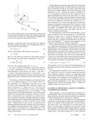
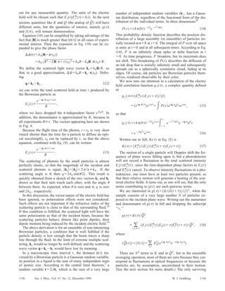
Dynamic light scattering

Dynamic light scattering
W. I. Goldburg
Citation: American Journal of Physics 67, 1152 (1999); doi: 10.1119/1.19101
View online: https://doi.org/10.1119/1.19101
View Table of Contents: http://aapt.scitation.org/toc/ajp/67/12
Published by the American Association of Physics Teachers
Articles you may be interested in
Theory of dynamic light scattering from polydisperse systems
The Journal of Chemical Physics 64, 2395 (1976); 10.1063/1.432528
Analysis of Macromolecular Polydispersity in Intensity Correlation Spectroscopy: The Method of Cumulants
A Study of Brownian Motion Using Light Scattering
American Journal of Physics 38, 575 (1970); 10.1119/1.1976408
Interactions in undersaturated and supersaturated lysozyme solutions: Static and dynamic light scattering results
The CONTIN algorithm and its application to determine the size distribution of microgel suspensions
Equilibrium time correlation functions and the dynamics of fluctuations
American Journal of Physics 67, 1161 (1999); 10.1119/1.19102

Dynamic light scattering
W. I. Goldburg
Department of Physics and Astronomy, University of Pittsburgh, Pittsburgh, Pennsylvania 15260
͑Received 27 May 1999; accepted 27 July 1999͒
By scattering light from small particles, their geometrical structure and their state of motion can be
measured. An experiment is described for measuring the diffusivity of small particles undergoing
Brownian motion using the technique called photon correlation spectroscopy or dynamic light
scattering. The necessary experimental apparatus and the related theory are discussed. Photon
correlation spectroscopy is a powerful tool for studying the dynamical behavior of fluids near
critical points, and a discussion is given of this phenomenon. The same experimental technique also
can be used to study laminar or turbulent flows, and the associated theory is introduced to enable
such experiments to be interpreted. © 1999 American Association of Physics Teachers.
I. INTRODUCTION
Fractals, continuous phase transitions, spinodal decompo-
sition, Brownian motion, the Wiener–Khinchine theorem,
the Brown–Twiss effect, photon correlation spectroscopy,
and turbulence. Many phenomena and ideas of great impor-
tance in statistical and condensed matter physics can be in-
troduced by studying dynamic light scattering. The goal of
this paper is to introduce this technique by describing a few
experiments that can be performed by undergraduate stu-
dents. The experimental possibilities are sufficiently rich that
they can be stimulating to graduate students as well. The
measurements require inexpensive optical components such
as a small He–Ne laser ͑output power of a few mW͒, a few
lenses and lens holders, and a photodetector. In addition, a
more expensive device is needed, namely a photon cor-
relator. Many correlators that may have been discarded by
researchers may serve the purpose perfectly well.1
A new
correlator can be purchased for several thousand dollars.
Considerable emphasis is placed on the Brownian motion
of micron-size particles diffusing in a background fluid such
as water, because an understanding of Brownian motion
opens the door to understanding a broad range of subjects,
including the dynamical behavior of fluids and fluid mix-
tures, and magnetic materials near their respective critical
points.
Near the critical point of fluids, we can observe fluctua-
tions by eye and also by using a very small laser. Section II
describes a desktop experiment for doing so. It turns out that
these fluctuations produce the same effects as those seen in
the scattering of light by small particles in Brownian motion.
Readers who have only a qualitative interest in light scatter-
ing can skip directly to Sec. II. The remainder of the paper is
intended for readers who are interested in setting up their
own apparatus to study Brownian motion or fluid dynamics
quantitatively. The same equipment can be used to make
measurements in fluids near the critical point.
Suppose that the experimental components have been as-
sembled and arranged on a table as indicated in Fig. 1. The
beam of the low-power He–Ne laser is directed at a small
vial or test tube filled with water in which small particles
have been suspended. For the particle suspension, a drop of
skim milk in water will do, but it is best to use particles, all
of which have the same diameter d in the 0.01 micron to 50
micron range.2
With the proper particle concentration, the
sample will be pale blue when viewed in room light. A laser
beam passing through the sample should appear as a bright
line which is well defined throughout the entire scattering
volume.
The experimental setup in Fig. 1 shows a photodetector
that collects light at a scattering angle ␪ equal to 90°. To
satisfy the spatial coherence condition discussed below the
distance R between the center of the sample cell and the
photodetector should be large; say, 30–100 cm. In addition,
a small pinhole of diameter h should be placed close to the
photodetector face. It is helpful to mildly focus the incident
laser beam on the sample volume, using, say, an fϭ20 cm
lens. Ideally, the scattering particles will produce a sharply
defined bright line in the fluid. Only a segment of the scat-
tered beam should fall on the face of the photodetector. This
segment can be defined by a pair of parallel closely spaced
black masking tape strips placed on the sample tube ͑sepa-
ration of the order of a mm͒. Alternatively, a lens can be
used to form the image of the scattering volume on a slit of
adjustable width L. The photodetector then accepts light
from scattering particles within the segment. Spatial coher-
ence is achieved by choosing h, L, and R to satisfy the
condition
BϭhL/R␭Շ1. ͑1͒
where ␭ is the wavelength of light in the water sample of
refractive index n, and ␭ is related to the vacuum wave-
length of the laser beam ␭vac by ␭ϭ␭vac /n. For water n
ϭ1.3.3
The optical coherence condition in Eq. ͑1͒ is familiar
from elementary optics. When Eq. ͑1͒ is satisfied, the photo-
detector collects light from only the first diffraction maxi-
mum produced by a slit of width L. For studies of Brownian
motion, one might want to choose L, R, and h so that B is
less than 10 or so ͑for studies of fluid motion discussed in
Sec. IV, B should be less than unity͒.
The photodetector should be operated as a pulse counting
device rather than in an analog mode, that is, it should sense
the individual photoelectron pulses. The width of these
pulses is not relevant to the experiment; only their spacing in
time is important. It is preferable if all the photopulses are of
the same width and amplitude, which is accomplished by
passing the photodetector output through a discriminator.
The individual pulses coming out of the discriminator should
be less than 1 ␮s in width and ideally less than 0.1 ␮s. Many
photodetectors come with a built-in discriminator with a
TTL output.
1152 1152Am. J. Phys. 67 ͑12͒, December 1999 © 1999 American Association of Physics Teachers

To be sure that all the optics and electronics are arranged
correctly, it is useful to observe the chain of TTL pulses on
an oscilloscope before sending them to the correlator. If the
TTL pulse width is shorter than 0.1 ␮s, use very short inter-
connecting cables or be sure that all outputs and inputs are
terminated in the characteristic impedance of the cable,
which is 50 ⍀ for RG58U cable. This is to avoid reflection of
pulses from the ends of the cable due to impedance mis-
matching problems. Data collection will be tedious if the
mean photon counting rate ͗I͘ is less than 1000 counts/s.
Figure 2͑a͒ shows a chain of photodetector pulses pro-
duced by incoherent light falling on the photodetector. The
pulses occur at random times, with their mean spacing being
inversely proportional to ͗I͘. Figure 2͑b͒ shows the detector
output from light that is scattered by diffusing particles in the
sample. In both experiments the photon pulses have passed
through a discriminator, assuring that all the pulses have the
same height and width. In Fig. 2͑b͒ the pulses are correlated
in time, that is, they are bunched together within a correla-
tion time ␶c which is determined by the diffusion coefficient
of the particles and the scattering angle. The photon cor-
relator identifies this clustering effect by measuring the cor-
relation function
K͑␶͒ϭ͗I͑t͒I͑tϩ␶͒͘ ͑2͒
or its dimensionless counterpart
g͑␶͒ϭ͗I͑t͒I͑tϩ␶͒͘/͗I͑t͒͘2
. ͑3͒
Experimentally, the average designated by the brackets in
Eq. ͑3͒ is a time average over the data collection interval T:
K͑␶͒ϭ
1
T
͵0
T
I͑t͒I͑tϩ␶͒dt, ͑4͒
where T typically ranges from seconds to many minutes,
with the choice dictated by the desired signal-to-noise ratio.
The mean intensity is the time average, ͗I͘
ϭ(1/T)͐0
T
I(t)dt.
In the experiments discussed here, the system is in thermal
equilibrium, or as in Sec. V, in a stationary state. In either
case ͗I(t)͘ϭ͗I(tϩ␶)͘, a fact that will be invoked repeat-
edly. Of course, K(␶) is not independent of ␶; its
␶-dependence is what we are interested in measuring and
calculating. Its characteristic decay time will be denoted as
␶c . Typically ␶c is in the range of hundreds of microseconds
to milliseconds, depending on the particle size used.
The signal-to-noise ratio, S/N, will always improve if the
data collection time T is increased. Suppose that we are con-
tent with data for which g(␶) is measured within 1%. First
assume that the counting rate ͗I͘ is so large that the quality
of the measurements is not determined by the low counting
rate, but is limited by the number NcϭT/␶c , of ‘‘fluctua-
tions’’ collected in the time T. According to Poisson
statistics,4
S/Nϭ1/ͱNc , and hence, one percent accuracy is
achieved by setting T/␶cϭ104
.
Next consider the opposite limit where the scattered inten-
sity ͗I͘ is very low. In this limit, the fluctuations in g(␶) will
be governed by so-called shot noise and will vary as the
inverse square root of the measuring time T. In this low
counting rate limit, where Poisson statistics is again relevant,
T/␶c is no longer the controlling parameter; to make a mea-
surement to 1% accuracy, choose T͗I͘ϭ104
.
Figure 3 shows a measured g(␶) produced by small par-
ticles in Brownian motion. The solution in which they are
Fig. 1. Experimental setup for studying the Brownian motion of particles in
water. The sample is labeled S. The laser L directs the incident beam ver-
tically upward. The photodetector PD converts the scattered light into a
pulse string which is fed to the correlator COR.
Fig. 2. ͑a͒ The output of the PD for immobile scatterers, as might be the
case if the sample has been frozen or if the sample is a piece of milk glass
or even a piece of paper. The arrival time of the photopulses is purely
random in this case. ͑b͒ The PD output of moving particles which are Dop-
pler shifting the frequency of the incident light. Note that the pulses tend to
cluster in time. This clustering time or correlation time ␶c is inversely pro-
portional to the diffusivity of the randomly moving particles that scatter the
light.
Fig. 3. Plot of g(␶) versus ␶ measured in a soap film which was only a few
␮m thick. The soap solution was a 1% dish washing detergent in water. The
seed particles were polystyrene spheres of diameter 1 ␮. Note that g(0)
Ӎ2.
1153 1153Am. J. Phys., Vol. 67, No. 12, December 1999 W. I. Goldburg

moving is a soap film only a few ␮m thick. For spherical
Brownian particles diffusing in the background solvent, it
can be shown4
that the function
G͑␶͒ϵg͑␶͒Ϫ1 ͑5͒
decays exponentially, with the decay rate given by
␶c
Ϫ1
ϭ2 Dq2
. ͑6͒
Here D is the diffusion coefficient of the particles and q is
the scattering wavevector whose magnitude q is given by
qϭ͉q͉ϭ
4␲
␭
sin
␪
2
, ͑7͒
where ␪ is the scattering angle and ␭ is ␭vac /n.
In a time t a particle will diffuse a mean square distance
͗r2
͘ that is proportional to Dt. The diffusion produces a
large fluctuation in the intensity in a time tЈ such that tЈ
Ӎ1/(Dq2
). This characteristic time tЈ is of the order ␶c . It is
these intensity fluctuations that a photon correlator measures.
Helpful discussions of diffusion can be found in Refs. 4 and
5.
The diffusion coefficient D depends on the particle diam-
eter d. For spherical particles, DϭkBT/3␲␩d,6
where T is
the temperature, kB is Boltzmann’s constant, and ␩ is the
viscosity of the background fluid. From this relation, we
have ␩ϭ0.01 g cmϪ1
sϪ1
and Dϭ4.4ϫ10Ϫ9
cm2
/s for a dif-
fusing particle 1 ␮m in diameter in water at room tempera-
ture. From a measurement of g(␶), we can obtain ␶c
Ϫ1
and
find the radius of the diffusing particles, even if they are too
small to be observed with a microscope. ͑See Fig. 4.͒ Simi-
larly, a measurement of g(␶) enables us to measure the ra-
dius of gyration of polymer molecules diffusing in solution
and to determine the correlation length of fluctuations in den-
sity or concentration in a fluid or mixture near its critical
point.7,8
Measurements of g(␶) can be a powerful tool for
studying phenomena that have nothing to do with diffusion,
for example, the determination of the width of a narrow
spectral line9
or the diameter of a distant double star.10
The
latter experiment gave birth to the technique of photon cor-
relation spectroscopy.
All photodetectors generate output pulses even when there
is no light shining on them. This dark count rate can be a few
Hz to several kHz. Except at very small ␶, these dark count
pulses occur roughly randomly in time and hence give a flat
background to g(␶), reducing the relative contribution of
G(␶), the quantity in which we are really interested. In room
light the photodetector will have the same effect. It is there-
fore necessary to employ a laser-generated counting rate that
is many times larger than the dark count rate and room light
count rate, in addition to satisfying the condition ͗I͘␶cӷ1.
The contribution to ͗I͘ from room light can be reduced by
placing an inexpensive interference filter11
directly in front
of the photodetector and interposing a tube between it and
the sample. A cardboard tube works well. For the most
noise-free results, turn off the room lights when the cor-
relator is making measurements.
If a flowing fluid is seeded with small particles, we can
learn a lot about the flow by measuring g(␶). The fluid flow
problem is treated in Sec. V. It will be seen that g(␶) gives
information about velocity differences between pairs of
points in the flow. Laminar and turbulent flows can be stud-
ied in the laboratory12–14
using the same apparatus as that
employed in the Brownian motion measurements.
In Sec. III the intensity correlation function is calculated
for a single Brownian particle, with the assumption that the
photodetector is so small that the scattering wave vector q is
sharply defined. The calculation will be valid even when
many particles are present in the sample, as long as they are
sufficiently far apart that they do not interact. We will see
that when B is no longer very small, G(␶) is diminished by
a factor f(A) which takes into account the fact that photons
scattered from the most widely separated diffusing particles
in the sample will interfere with each other to give
G͑␶͒ϭg͑␶͒Ϫ1ϭf͑A͒eϪ2Dq2␶
. ͑8͒
The argument A in f(A) is the area of the photodetector, an
important parameter in the subsequent calculation of f(A) in
Sec. IV.
The single-particle calculation of g(␶) is presented in Sec.
III. To find f(A) in Eq. ͑8͒, we must consider the motion of
many Brownian particles, because its attenuating effect
arises from the interference of the electric fields scattered by
these particles. The calculation of f(A) appears in Sec. IV.
The basic theory developed in Secs. II and III can be ap-
plied with little modification to the study of laminar and
turbulent flows, which is the subject of Sec. V. Some con-
cluding remarks are given in Sec. VI.
II. CRITICAL PHENOMENA, LIGHT SCATTERING,
AND BROWNIAN MOTION
Light scattering is a very powerful tool for studying criti-
cal phenomena. Some of the central features of continuous
phase transitions are easily observed and can be presented in
a lecture demonstration or observed on a desktop.
Here we briefly review the subject of critical phenomena
and describe an experiment for observing a striking manifes-
tation of it, namely critical opalescence. You can observe
this effect with a very small laser of the type used as a
pointer in lecture halls. In addition, you will need a small
glass container to hold the sample, which might be a mixture
of 2,6-lutidine and water ͑LW͒, available from a chemical
supply house. A convenient sample cell is a vial of diameter
Fig. 4. Sketch of diffusing particle with an incident beam traveling from left
to right. The particle is located at the origin of the coordinate system at time
tϭ0 and at time t its position is r(t). The photodetector is labeled PD. The
directions of the incident and scattered beams are shown.

Ϸ1 cm and a height of several centimeters. The vial should
have a good screw top, because 2,6-lutidine15
has a very
unpleasant smell. The trick is to prepare the LW mixture so
that the lutidine concentration c is close to the critical con-
centration, cc , which is 28% by weight. In a binary mixture
such as LW, the concentration variable plays the same role
as the density in a simple fluid such as water or CO2.16
Sample preparation should be carried out under a hood or
in a very well ventilated space. After the water and lutidine
have been placed in the container with its composition within
a few percent of cc and shaken up, it will be in one phase if
the temperature is less than the critical temperature, Tc
ϭ33.4 °C. Place the cell in a beaker of water, which will
serve as a temperature bath. The bath is then heated by add-
ing hot tap water. When the sample is held for a few minutes
at a high temperature well above Tc , it will separate into two
well-defined phases, with the heavier water-rich phase on the
bottom.
If you were successful in preparing a sample close to the
critical concentration, the volumes of the two phases will be
almost equal. If not, insert a syringe into the cell and draw
out the excess phase ͑or add a drop or two of the appropriate
minority component͒, so that the two phases have equal vol-
ume. After this single iteration, you have probably prepared
the mixture adequately close to Tc .
To observe critical opalescence, return the sample cell to
the water bath and heat it slowly, shaking the sample cell
now and then to bring the mixture to the same temperature as
that of the surrounding bath. When T is increased through Tc
from below, droplets will form, and after several minutes,
the more dense water-rich phase will settle to the bottom and
two sharply defined phases will be seen. The most instructive
observations are made when the system is still in one phase,
so increase the bath temperature slowly as Tc is approached.
When the temperature becomes close to Tc , the sample
will develop a brownish appearance because it is strongly
scattering the room light. The scattering may become so
large that the laser beam, which you should now be sending
through the sample, may hardly go through it. This phenom-
enon is called critical opalescence. Place a sheet of paper so
that you can view the transmitted beam. You should see that
the scattered light consists of speckles that flash on and off in
a random fashion.
How are we to understand this strong scattering phenom-
enon when the system is in one phase but close to Tc? Near
the critical point, small regions of water rich and lutidine rich
phases momentarily form and then diffuse away. This same
phenomenon occurs far from the critical point, but the size of
the regions is much smaller than the wavelength of light, and
the regions come and go so quickly that most measuring
instruments will not be able to record them. Similarly, a
glass of water near room temperature undergoes fluctuations
in density, but these fluctuations are so small in spatial extent
and in amplitude that they cannot be easily observed. More-
over, the fluctuation rate ⌫ is very fast far above or below
Tc , because small-scale density variations diffuse away
faster than large ones, making them unobservable by eye and
even by very fast electronic equipment.
Near the critical point, the free energies of the one-phase
states and the two-phase states are almost the same. As a
result, the system makes brief excursions or fluctuations
from the one-phase state to the two phase state, that is, it
locally tries to phase separate, even though the system is
globally in one phase. These local fluctuations in density or
composition produce local variations in the refractive index
n. It is these local variations in n that scatter the light, just as
a small lens would. As Tc is approached, these composition
fluctuations grow in magnitude and in spatial extent ␰ and
can become even larger than the wavelength of light. The
fluctuations of size ␰ cause G(␶)ϭg(␶)Ϫ1 to vary as
eϪ2Dq2t
, just as for Brownian particles ͑provided q␰Ͻ1).
The diffusivity D in G(␶) is the same as that of a Brownian
particle, except that the radius d/2 of the diffusing particle is
replaced by ␰.
The reader interested in learning more about critical phe-
nomena and the role of light scattering has many sources of
information available, such as those collected in Refs. 8, 16,
and 17.
III. INTENSITY CORRELATION FUNCTION FOR
BROWNIAN PARTICLES
We first deduce the limiting value of g(␶) for ␶ӷ␶c . In
this limit the intensities at t and tϩ␶ are unrelated, so
K(␶)ϭ͗I(t)͗͘I(tϩ␶)͘→͗I(t)͘2
ϭ͗I(tϩ␶)͘2
in steady or
equilibrium states. Therefore g(␶→ϱ)ϭ1 in Eq. ͑3͒.
In the opposite limit ␶Ӷ␶c , the scattered intensities at the
times t and tϩ␶ are almost equal, so that g(␶)→͗I2
͘/͗I͘2
,
which is in general greater than unity. For the Brownian
motion problem, we will see that g(␶→0)ϭ2. If the sample
contains large specks of dust that produce occasional bright
flashes of light when floating through the laser beam, we are
no longer dealing with the Gaussian statistics of Brownian
motion, and g(0) can greatly exceed two.
We are interested in g(␶) generated by non-interacting
Brownian particles such as polystyrene latex spheres of di-
ameter dϭ1 ␮m in a small container of water. As a starting
point, consider a particular particle located at r(t) at time t
that was at r(0) at tϭ0. A laser beam traveling along the y
axis illuminates the particle, which then scatters the incident
beam. The photodetector, which is located a large distance R
from the origin, senses the scattered field, producing photo-
pulses at the ͑fluctuating͒ counting rate I(t). The intensity
I(t) is proportional to the square of the incident electric field
Ei , which is assumed to be of complex form:
EiϭE0eϪiki•r(t0)ϩi␻t0, ͑9͒
where ␻ is an optical frequency of the order of 1015
Hz and
t0 is the instant when the scattered wave leaves the particle.
Here ki has the direction of the incident beam and its mag-
nitude is k0ϭ2␲/␭. Because we are ultimately interested in
the ratio of scattered intensities, nothing is lost by taking this
field to be expressed in dimensionless units. The scattered
field Es is a spherical wave whose amplitude is proportional
to the incident field amplitude:
Es͑R,t͒ϰ
Ei͑t0͒eϪik0͉RϪr(t0)͉
͉RϪr͑t0͉͒
ei␻(tϪt0)
. ͑10͒
The intensity is
I͑t͒ϭConst Es͑R,t͒Es*͑R,t͒. ͑11͒
The constant of proportionality depends on many param-
eters, including E0 and R. The factor ei␻t
in Eq. ͑10͒ will
sometimes be suppressed because it will always be canceled

out for any measurable quantity. The units of the electric
field will be chosen such that Es(t)Es*(t)ϭI(t). In the next
section, quantities like K and Q ͑the analog of Q˜ ) will have
different units, but the quantities of interest, namely g(␶)
and f(A), will remain dimensionless.
Equation ͑10͒ can be simplified by taking advantage of the
fact that ͉R͉ is much greater than ͉r(t)͉ in all cases of experi-
mental interest. Then the exponent in Eq. ͑10͒ can be ex-
panded to give the phase factor
⌬␾͑t͒ϭk0͉RϪr͑t0͉͒
ϭk0ͱR2
Ϫ2R•rϩr͑t0͒2
Ӎk0RϪk0R•r͑t0͒/R.
We define the scattered light wave vector ksϭk0R/R, so
that, to a good approximation, ⌬␾ϭk0RϪks•r(t0). Defin-
ing
qϭksϪki , ͑12͒
we can write the total scattered field at time t produced by
the Brownian particle as
Es͑t͒ϰ
eϪiq•r(t0)ϩi␻t
R
,
where we have dropped the r-independent factor eik0R
. In
addition, the denominator is approximated by R, because in
all experiments Rӷr. The vectors appearing here are shown
in Fig. 4.
Because the flight time of the photon, tϪt0 is very short
͑much shorter than the time for a particle to diffuse an opti-
cal wavelength͒, t0 can be replaced by t, so that the above
equation, combined with Eq. ͑9͒, can be written
Es͑t͒ϰ
eϪiq•r(t)ϩi␻t
R
. ͑13͒
The scattering of photons by the small particles is almost
perfectly elastic, so that the magnitude of the incident and
scattered photons is equal, ͉ks͉ϭ͉ki͉ϭ2␲/␭ϵk0 . If the
scattering angle is ␪, then qϭ2k0 sin(␪/2). This result is
quickly obtained from a sketch of the two vectors ks and ki
drawn so that their tails touch each other, with the angle ␪
between them. As expected, when ␪ is zero and ␲, q is zero
and 2k0 , respectively.
In this discussion, the vector nature of the electric field has
been ignored, so polarization effects were not considered.
Such effects are not important if the refractive index of the
scattering particle is close to that of the surrounding fluid.18
If this condition is fulfilled, the scattered light will have the
same polarization as that of the incident beam, because the
scattering particles behave almost like point dipoles, their
dipole moment being induced by the incident electric field.19
The above derivation is for an ensemble of non-interacting
Brownian particles, a condition that is well fulfilled if the
particle density is low enough that the beam traces a sharp
line through the fluid. In the limit of extreme multiple scat-
tering, ks would no longer be well-defined, and the scattering
wave vector qϭksϪki would have lost its meaning.
In a macroscopic time interval t, the distance r(t) tra-
versed by a Brownian particle is a Gaussian random variable;
its position in a liquid is the sum of many independent steps
of atomic size. According to the central limit theorem,5
a
random variable rϭ͚␦ri which is the sum of a very large
number of independent random variables ␦ri , has a Gauss-
ian distribution, regardless of the functional form of the dis-
tribution of the individual terms. In three dimensions20
P͑r͒ϭ͑4␲Dt͒Ϫ3/2
eϪr2/4Dt
. ͑14͒
This probability density function describes the position dis-
tribution of a large assembly ͑or ensemble͒ of particles ini-
tially located at rϭ0 at tϭ0. The integral of P over all space
is unity at tϭ0 and at all subsequent times. According to Eq.
͑14͒, P is an infinitely sharp spike or delta function at t
ϭ0. As time progresses, P broadens, but its maximum does
not shift. This broadening of P(t) describes the diffusion of
an ink drop that is initially infinitely small and subsequently
spreads out as a spherically symmetric cloud, fading at its
edges. Of course, ink particles are Brownian particles them-
selves, rendered observable by their color.
We now turn our attention to a calculation of the electric
field correlation function g1(␶), a complex quantity defined
as
g1͑␶͒ϵ͗Es*͑t͒Es͑tϩ␶͒͘/͗I͘
ϭ͗eiq•r(␶)
͘ei␻␶
ϭ ͵P͑r͒eiq•r
d3
rei␻t
, ͑15͒
so that
g1͑␶͒ϭ͑4␲D␶͒Ϫ3/2
ei␻␶
͵Ϫϱ
ϱ
eϪr2/2D␶
eϪiq•r
d3
r
ϭeϪDq2␶
ei␻␶
. ͑16͒
Written out in full, K(␶) in Eq. ͑2͒ is
K͑␶͒ϭ͗Es*͑t͒Es͑t͒Es*͑tϩ␶͒Es͑tϩ␶͒͘. ͑17͒
The motion of a single particle will Doppler shift the fre-
quency of plane waves falling upon it, but a photodetector
will not record a fluctuation in the total scattered intensity
Es(t)Es*(t), since the time-dependent phase factors in Es(t)
and Es*(t) cancel. To observe intensity fluctuations in a pho-
todetector, one must have at least two particles present, so
that their relative motion will generate a beating of the scat-
tered electric fields. It turns out, as one will see, that the only
terms contributing to g(t) are such pairwise terms.
We are interested in g(␶)ϭ͗I(t)I(tϩ␶)͘/͗I͘2
, when the
sample consists of a very large number N of particles ex-
posed to the incident plane wave. Writing out the numerator
and denominator of g(␶) in full and dropping the subscript
‘‘s,’’
g͑␶͒ϭK͑␶͒/Q˜ 2
ϭ ͚i,j,k,l
͗Ei͑t͒Ej*͑t͒Ek͑tϩ␶͒El*͑tϩ␶͒͘/Q˜ 2
, ͑18͒
where
͗Q˜ ͑t͒͘ϭ͗I͑t͒͘ϭ͚i,j
E0
2
͗ei(q•ri(t)
eϪi(q•rj(t)
͘.
There are N4
terms in K and in Q˜ 2
, but in the ensemble
averaging operation, most of them are zero because they cor-
respond to fluctuations at optical frequencies or because the
particles are, by assumption, uncorrelated in their motion.
͑See the next section for more details.͒ The only surviving

terms are those for which iϭl and jϭk. The absence of a
correlation between the particles enables one to factor func-
tions like ͗Ei(t)El*(tϩ␶)Ej*(t)Ek(tϩ␶)͘ into the product of
pairwise correlation functions with iϭl and jϭk, so that this
product may be written ͗Ei(t)Ei*(tϩ␶)͗͘Ej*(t)Ej(tϩ␶)͘
with i j. Because all particles scatter identically, this term
has the same value as ͉͗Ei(t)Ei*(tϩ␶)͉͘2
, even though it
represents a beating term between different particles i and j.
There will be N2
ϪNӍN2
such electric field correlation
function terms in K(␶).
Now consider those terms for which iϭj and kϭl,
namely ͚i,j͗Ei(t)Ei*(t)Ej(tϩ␶)Ej*(tϩ␶)͘. It is equal to
N2
E0
2
ϭ͗I͘2
, or equivalently N2
͉͗E(t)͉͘2
, where E is the
field scattered by a single particle.
Collecting these results and putting them in Eq. ͑15͒ per-
mits one to write
g͑␶͒ϭ1ϩ͉͗͑E͑t͒E*͑tϩ␶͉͒͘2
/͉͗E͑t͉͒2
͉͘2
. ͑19͒
Or equivalently,
g͑␶͒ϭ1ϩ͉g1͑␶͉͒2
. ͑20͒
The correlation function is written in the above way be-
cause the result holds more generally than suggested by this
derivation; Eq. ͑20͒ is valid for any N-particle system, as
long as the the total scattered field, Esϭ͚jEj is a ͑two-
dimensional͒ Gaussian random variable. This important
equation is called the Bloch–Siegert theorem. Its full deriva-
tion can be found in Ref. 21.
Because ͉͗E*(t)E(tϩ␶)͘/͉͗E(t)͉2
͘2
ϭeϪ2Dq2␶
, we have,
g͑␶͒ϭ1ϩeϪ2Dq2␶
, ͑21͒
which is our central result.
Equation ͑21͒ gives the correct ␶ dependence of G(␶)
ϭg(␶)Ϫ1, even when B is large and f(A) in Eq. ͑8͒ is
correspondingly small. On the other hand, it fails when ap-
plied to flowing fluids, where the particles are no longer
moving independently. In that case, the factorization of the
fourfold correlation function in K(␶) is no longer permis-
sible, and one must turn to the formalism presented in Sec.
V.
For a sample containing a spread of particle diameters,
such as dilute milk, g(␶) will consist of a sum or integral of
exponentially decaying contributions of the form
eϪ2Di(d)q2␶
, with each term appropriately weighted by a con-
centration factor ci(d). There exists a large body of literature
dealing with this weighting problem, as it is of great practical
importance.22
Further complications arise if the Brownian
particles are not spherical in shape.7
So far we have considered only the limit BӶ1, so that the
photodetector is receiving light from a single scattering vec-
tor, ks . That restriction is lifted in the next section. In many
experiments, the finite area of the photodetector changes
only the amplitude of G(t), but for fluid flow, the shape of
this function can be appreciably changed if B is not less than
unity.12,13
IV. THE EFFECT OF SPATIAL INCOHERENCE
The goal of this section is to calculate the ͑de͒coherence
factor f(A) in Eq. ͑8͒. This function will depend on the
precise shape and size of the source as seen by the photode-
tector and on the same parameters for the photodetector sur-
face with area A. Consider the special geometrical arrange-
ment shown in Fig. 5. The wave number ki of the incident
laser beam has been chosen to lie in the plane of the paper,
and the photodetector receives light from a range of ks val-
ues. The mean value of the scattered wavevector ͗ks͘ points
along the z axis in Fig. 5, so the average scattering vector q
is given by qϭ͗ks͘Ϫki . Its direction and magnitude are
shown in Fig. 5.
The rectangular coordinate system is centered at a point
near the center of the sample. Another coordinate system xЈ,
yЈ, zЈ is also employed. The origin of this coordinate system
is at the geometrical center of the photodetector; its face is
assumed to be square, with dimensions h. If the photosensi-
tive area is circular, its radius is also taken to be h.
The detector collects light from a range of scattered vec-
tors ks , and the photon momentum transfer is designated as
⌬kϭksϪkiϭqϩ␦k. ͑22͒
For the jth particle the scattered electric field is
EjϭE0eϪi⌬k•rj(t)ϩi␻t
. ͑23͒
The subscript ‘‘s’’ in the scattered field has now been
dropped. It will be assumed, as before, that all scattering
particles have the same diameter, so that the scattering am-
plitude E0 is common to all of them. Therefore it does not
appear in g(␶), and we set it equal to unity.
The correlation function K(␶) in Eq. ͑8͒ is the product of
four electric field factors, each of which is now a sum over
all N particles in the sample. The scattered photons will go to
all points on the face of the photodetector, and for each
point, the momentum transfer ⌬k will be different. We need
to sum over all such points or rather integrate over the pho-
tosensitive area A.
At time t, the product Ei(t)Ej*(t) will contain terms such
as ei(qϩ␦k)•(rj(t)Ϫri(t))
, where we have replaced ⌬k by its
equivalent, qϩ␦k. In writing this expression, it has been
recognized that to a very good approximation qϩ␦k is inde-
Fig. 5. Schematic diagram showing the scattering geometry and the coordi-
nate directions discussed in Sec. IV. The incident beam ki , like all the other
wave vectors shown, lies in the plane of the paper. The scattering wave
vector ͑or the momentum transfer͒ for the photon striking the photodetector
surface at the point (xЈϭ0,yЈ) is ⌬kϭksϪkiϭqϩ␦k. Here q is the aver-
age value of ⌬k. In the detailed calculations presented here, the incident
beam is travelling in the Ϫy direction, and the photodetector is a square of
area hϫh or a circle of diameter h. A second coordinate system xЈ, yЈ, zЈ
is at the geometrical center of the photodetector.

pendent of the particle positions rn(t), so this momentum
change is independent of particle position in the sample.
The notation is simplified by letting rijϭrj(t)Ϫri(t). In
the short time interval ␶, particles i and j change their rela-
tive positions by a distance ␦rij(␶), so at time tϩ␶, the
difference in positions of this particle pair is rij(t)ϩ␦rij .
Integrating the scattered intensity over the area of the photo-
detector for both I(t) and I(tϩ␶), we obtain
g͑␶͒ϭK͑␶͒/Q2
ϭͳ͵A
I͑t͒dAЈ͵A
I͑tϩ␶͒dAЈʹͲQ2
, ͑24͒
where
Q͑t͒ϭͳ͵A
I͑t͒dAЈʹϭͳ͚i,j
͵A
ei(qϩ␦k)•rij(t)
dAЈʹ
ϭ͚i,j
ͳ͵A
ei(qϩ␦k)•rij(t)
dAЈʹ.
͑25͒
The summations and integrations are freely interchanged
here.
Writing out K(␶) in full, we have
K͑␶͒ϭ͚i,j
ͳ͵A
ei[(qϩ␦k)•rij(t)]
dAЈ
ϫ͚l,m
͵A
eϪi(qϩ␦k)•[rlm(t)ϩ(␦rlm(␶)]
dAЈʹ. ͑26͒
Remember that each little area element dA on the face of the
photodetector has a different ␦k associated with it. This fact
will be used when we come to evaluate this integral in two
spatial cases: a square and a circular photodetector.
Because the particles have random positions at all times,
the ensemble average implied by the brackets, will give zero
contribution to Q unless iϭj and in that case, rij(t)ϭ0.
Thus QϭNA and
Q2
ϭN2
A2
. ͑27͒
For K(␶), we have no such simplification. Every term in Eq.
͑26͒ not involving ␦k can be taken out of the integral, so that
this equation can be written in full as
K͑␶͒ϭ ͚i,j,l,m
͗eiq•(␦rl(␶)Ϫ␦rm(␶))
eϪiq•(rjϪriϩrlϪrm)
BlmCij͘,
͑28͒
where, for any i and j
Cijϭ ͵A
ei␦k•rij dAЈϭCji* ͑29͒
and
Blmϭ ͵A
ei␦k•(rlm(t)ϩ␦rlm(␶))
dAЈ. ͑30͒
For every particle pair, the relative change in the particle
positions ␦rlm(␶) is small compared to their separation
rlm(t), so we can set ClmϭBlm . Also, the randomness of the
particle positions again allows us to simplify the expressions;
the only terms in Eq. ͑28͒ that will not average to zero are
those for which iϭj and lϭm or iϭl and jϭm. For these
terms (rjϪriϩrlϪrm) in Eq. ͑28͒ is zero.
Because N is typically very large, we can neglect the N
terms for which iϭjϭlϭm, there being only N of these
terms compared to the N(NϪ1)ӍN2
particle pairs that do
not satisfy this fourfold equality. Taking advantage of this
fact, we write
K͑␶͒ϭN2
A2
ϩ ͚l,m l
͗eiq•[␦rl(␶)Ϫ␦rm(␶)]
ClmClm* ͘. ͑31͒
The first term on the right comes from setting iϭj and l
ϭm. Particles undergoing Brownian motion are uncorre-
lated, so we can write
K͑␶͒ϭN2
A2
ϩN2
͗eiq•␦rlm(␶)
ClmClm* ͘
ϭN2
A2
ϩN2
͗ClmClm* ͗͘eiq•␦rml(␶)
͘. ͑32͒
We are justified in averaging the product ClmClm* ϭ͉Clm͉2
separately from the remaining phase factor term, because the
change in separation ␦rij(␶) in the interval ␶ has nothing to
do with the initial ͑random͒ separation rij(t) of the Brownian
particles. This major simplification is lost when the particles
are moving coherently, as discussed in Sec. V for fluid flow.
In the present notation, for any l
͗eϮiq•␦rl(␶)
͘ϭeϪDq2␶
, ͑33͒
and the independence of the motion of the particles permits
us to write
͗eiq•␦rml(␶)
͘ϭ͗eiq•␦rl(␶)
͗͘eϪiq•␦rm(␶)
͘. ͑34͒
Thus
K͑␶͒ϭN2
A2
ϩN2
͉͗Clm͉2
͘eϪ2Dq2␶
. ͑35͒
Dividing by Q2
ϭN2
A2
from Eq. ͑28͒ gives the result we
seek for the case of ͑uncorrelated͒ Brownian motion of par-
ticles in the sample:
g͑␶͒ϭ1ϩf͑A͒eϪ2Dq2␶
, ͑36͒
where f(A)ϭ͉͗Clm͉2
͘/A2
.
The function Clm depends on the particle separations rlm ,
and for all applications of interest, we can treat this separa-
tion as a continuous variable. Then Clm can be replaced by
C(r) where r is the separation of pairs of diffusing particles.
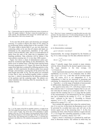
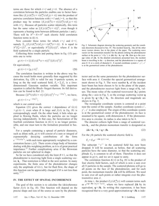
We must integrate over all r lying in the sample volume. In
addition, there is an integration over the face xЈ, yЈ of the
photodetector ͑see Fig. 5͒. For algebraic simplicity, we con-
sider the special case of the incident laser beam ki traveling
along the y axis and illuminating the Brownian particles over
the vertical distance 0рyрL. In the integration over the
illuminated sample volume, account must be taken of the
fact that there is a larger likelihood of finding a pair of par-
ticles separated by a short distance y, compared to the prob-
ability of encountering particles of separation slightly
smaller than L. Because the illuminated region is a thin ver-
tical line ͑see Fig. 5͒, the normalized probability density
function w(y) has a particularly simple form w(y)ϭ(2/L)
ϫ(1Ϫy/L) for a light source of length L.12,13
The reader is
reminded that y is a component of the separation of a pair of
particles and not the coordinate y in Fig. 5. In this case C(r)
is real and ͗C(r)C*(r)͘ϭ͐0
L
w(y)C(y)2
dy.
Before proceeding to the final integration that yields g(␶),
we simplify the exponent ␦k•r in the expression for C(r) in
Eq. ͑26͒. Assuming that the detector is square, has an area

hϫh, and its face is normal to the direction of ͗ks͘, the
scalar product in Eq. ͑24͒ is ␦k•rϭk0yyЈ/R. Then
C͑r͒ϭh ͵Ϫh/2
h/2
eik0yyЈ/R
dyЈϭ
h2
sin͑k0hy͒
k0hy
ϭh2
sinc͑k0hy͒.
͑37͒
We use Eq. ͑37͒ and the fact that Q2
ϭN2
h4
, because the
square photodetector has sides h, we have
f͑A͒ϭ ͵0
L
͑2/L͒͑1Ϫy/L͒sinc2
͑k0yh/R͒dy. ͑38͒
It has been implicitly assumed in the above calculation that
the incident laser beam has a square profile. In reality, laser
beams usually have radially Gaussian intensity variation.
This fact does not alter the above derivation as long as the
beam length L seen by the photodetector is long compared to
the Gaussian beam radius.
Consider next the case where the aperture in front of the
photodetector is circular with diameter a. Again the incident
laser beam is a thin line of light traveling along the y-axis in
Fig. 5. We switch to cylindrical coordinates, ␦ks•r
ϭk0ryyЈ/R, where ry is the component of source coordinate
r in the y direction. Taking a to be the diameter of the
detector, we obtain
C͑r͒ϭC͑ry͒ϭ ͵0
a/2
͵0
2␲
ei(k0ryrЈ/R)cos ␾
d␾ dry
ϭ2␲ ͵0
a/2
J0ͫk0ryrЈ
R ͬrЈ drЈ, ͑39͒
where Jn(u) is a Bessel function of order n. Using
͐0
u
J0(uЈ)uЈ duЈϭuJ1(u), we find
G͑␶͒ϭ4 ͵0
L
͑2/L͒͑1Ϫry /L͒
ϫ͓J1͑k0ary/2R͒/͑k0ary/2R͔͒2
dry eϪ2Dq2␶
ϭf͑A͒eϪ2Dq2␶
. ͑40͒
Again, f(A) falls below unity when B is no longer small,
because the photodetector is accepting light from many in-
dependently fluctuating speckles ͑intensity maxima͒, which
tend to average out the intensity fluctuations.
V. FLUID FLOW
We now ignore the effect of Brownian motion and instead
calculate G(␶) under conditions where the velocity is chang-
ing from point to point and is a function of time t. The above
derivation requires surprisingly little modification, even
though the functional form of G(␶) will be entirely different
when the particles in the flow are not moving independently.
The calculation will show that G(␶) decays in a time ␶c
governed by the velocity variation measured across L. Let
V(L) be the rms velocity difference across the source width
L. We will find that ␶cӍ(qV(L))Ϫ1
if BӶ1. If, on the other
hand, the photodetector collects light from many speckles,
the shape of G(␶) will be altered.
Again focus attention on a pair of particles, l and m, mov-
ing at velocities vl(t) and vm(t). We can replace ␦rij(␶), the
relative change in position of this particle pair in a time ␶, by
Vlm␶ϭ ͵t
tϩ␶
͓vl͑tЈ͒Ϫvm͑tЈ͔͒dtЈ. ͑41͒
We have used the fact that in the short time ␶ where G(␶) is
appreciable, the change in velocity difference Vlm is almost
constant. If the flow is turbulent, Vlm is a random variable as
measured in an experiment that spans many correlation times
in the measuring time T.
With this change, the above results can be used, except for
the fact that the factorization in Eq. ͑32͒ is no longer permis-
sible. Therefore we have
K͑␶͒ϭN2
A2
ϩ ͚i,j,i j
͗eiq•Vij␶
CijCij*͘. ͑42͒
Here there is no justification for averaging the factor CijCij*
separately. To understand this point, consider a pair of par-
ticles that are near each other in the source and another pair
that is widely separated. There will be a coherence factor B
associated with each of these pairs, because closely spaced
particles will produce a broader speckle than those that are
not, just as a narrow slit produces a broader diffraction maxi-
mum than does a wide slit. Thus, the widely spaced pair will
receive a smaller weight in G(␶). It is therefore necessary to
assure that BϭhL/R␭Ӷ1 if the measurements are to have a
reasonably direct interpretation. Reference 13 discusses a
calculation and a measurement of the effect on G(␶) when B
is not small, so that the photodetector collects light from
many speckles.
As before, the seeding density of the particles is assumed
to be sufficiently high that Vij can be replaced by V(r),
where r is the distance between a particle pair. Because V(r)
is a random variable that generally will not be Gaussian, the
probability distribution P must be left as an unknown func-
tion to be determined by the experiment. Let Vq(r) be the
component of the velocity difference V along q. We will see
that the measured G(␶) is closely related to the Fourier
transform of P(Vq). ͓If light is carried from the sample to
the photodetector by single-mode optical fibers, no integral
over A is required, and G(␶) and P(Vq) are cosine transform
pairs.23
͔.
By repeating the same steps needed to obtain G(␶) for
Brownian motion, we calculate that for a source in the form
of a thin line of length L and for a scattering angle of 90°,
G͑␶͒ϭ
1
A2 ͵Vq(r)ϭϪϱ
VqϭϪϱ
͵0
L
w͑r͒P͑Vq ,r͒
ϫcos͑qVq␶͉͒C͑r͉͒2
dVq͑r͒dr. ͑43͒
In Eq. ͑43͒ the exponential factor in Eq. ͑42͒ has been re-
placed by the cosine, because K(␶) is real.
For a photodetector with a square face of area hϫh,
G͑␶͒ϭ ͵0
L
͵Vq
͑2/L͒͑1Ϫy/L͒P͑Vq ,r͒cos͑qVq͑r͒␶͒
ϫ͓sinc͑k0hry/2R͔2
dVq͑r͒. ͑44͒
For laminar flows Vq is not a random variable and no
integration over dVq is necessary. For turbulent flows it has

not been possible to derive P(Vq ,r), even when the turbu-
lence is isotropic. For this reason the subject of turbulence
remains a very active one,24
to which the photon correlation
technique can be employed to advantage.
For a simple example of a laminar flow that is easily stud-
ied, consider the seeded sample to be cylindrical in shape
and rotating about its axis on, say a record turntable. Let its
angular frequency be ␻, so that the azimuthal velocity is
given by v␾ϭr␻. To avoid having to take into account
Brownian motion of the seed particles, one might want to
choose a solvent having a large viscosity, such as a mixture
of glycerine and water. This choice will make D small, so
that the decay term eϪ2Dq2␶
can be ignored. If parameters are
chosen to assure BӶ1, so that the factors C(r) can be ig-
nored as well, a simple integration of Eq. ͑43͒ establishes
that
g͑␶͒ϭ1ϩ͓sinc͑x͔͒2
, ͑45͒
where xϭqVq␶/2ϭk0L␻␶/2. The decaying oscillations of
this function are easily observed.
VI. CONCLUSION
Dynamic light scattering has long been a powerful tool for
studying a wide range of phenomena, only a few of which
have been discussed here. In these and many other applica-
tions, the scattering is generated by small particles that have
been introduced into a solvent, which is assumed to scatter
light weakly. But many fluid-like and glassy systems, such as
gels, strongly scatter light by themselves, so that no probe
particles need be introduced. The experiments suggested
here could easily provide a launching point for original in-
vestigations.
No mention has been made of the use of optical fibers to
couple the light from the source to the photodetector. With
this new technical development, dynamic light scattering ex-
periments become much more convenient. Because single-
mode fibers will conduct light having a single wavenumber,
we can satisfy the coherence condition BӶ1 without having
to put the photodetector and sample far from each other. A
useful introduction to this technique can be found in recent
work by Du et al.23
The measurements shown in Fig. 3 were
made with a relatively inexpensive optical fiber that did not
preserve polarization.
ACKNOWLEDGMENTS
I am especially indebted to P. Tong, K. J. Ma˚lo”y, and J. R.
Cressman for their contribution to my understanding of this
subject and to Rob Cressman and Quentin Bailey for their
careful reading of this paper. This work is supported by
grants from the NSF and NASA.
1
For example, older models of Malvern, Langley Ford, and Brookhaven
correlators should work fine.
2
A good source of such particles is PolyScience, 6600 W. Touhy Ave., P.O.
Box 48312, Niles, IL 60714.
3
D. Halliday, R. Resnick, and J. Walker, Fundamentals of Physics ͑Wiley,
New York, 1997͒, 5th ed., Chap. 37.
4
C. Kittel, Elementary Statistical Physics ͑Wiley, New York, 1958͒.
5
F. Reif, Fundamentals of Statistical and Thermal Physics ͑McGraw–Hill,
New York, 1965͒.
6
A. Einstein, in Investigations on the Theory of Brownian Motion, edited by
R. Furth and A. D. Cowper ͑Dover, New York, 1956͒, Chap. I.
7
B. J. Berne and R. Pecora, Dynamic Light Scattering ͑Wiley-Interscience,
New York, 1976͒.
8
W. I. Goldburg, ‘‘The dynamics of phase separation near the critical point:
spinodal decomposition and nucleation,’’ in Scattering Techniques Ap-
plied to Supramolecular and Nonequilibrium Systems, edited by S.-H.
Chen, B. Chu, and R. Nossal ͑Plenum, New York, 1981͒, pp. 383–409,
and other articles in this volume.
9
L. Mandel and E. Wolf, ‘‘Coherence Properties of Optical Fields,’’ Rev.
Mod. Phys. 37, 231–287 ͑1965͒.
10
R. Hanbury Brown and R. Q. Twiss, ‘‘Correlation between photons in two
coherent beams of light,’’ Nature ͑London͒ 177, 27–29 ͑1956͒.
11
Edmund Scientific in Barrington, NJ is a good source for interference
filters and other optical components.
12
P. Tong et al., ‘‘Turbulent transition by photon-correlation spectroscopy,’’
Phys. Rev. A 37, 2125–2133 ͑1988͒.
13
K. J. Ma˚lo”y et al., ‘‘Spatial coherence of homodyne light scattering from
particles in a convective velocity field,’’ Phys. Rev. A 46, 3288–3291
͑1992͒.
14
H. Kellay et al., ‘‘Experiments with Turbulent Soap Films,’’ Phys. Rev. A
74, 3975–3978 ͑1995͒.
15
Also called 2,6-dimethylpyridine.
16
H. E. Stanley, Introduction to Phase Transitions and Critical Phenomena
͑Oxford, New York, 1971͒.
17
W. I. Goldburg, ‘‘Light scattering investigations of the critical region in
fluids,’’ in Light Scattering Near Phase Transitions, edited by H. Z. Cum-
mins and A. P. Levanyuk ͑North-Holland, New York, 1983͒, pp. 531–581;
J. D. Gunton, M. San Miguel, and P. S. Sahni, Phase Transitions and
Critical Phenomena, edited by C. Domb and J. L. Lebowitz ͑Academic,
London, 1983͒, Vol. 8.
18
H. C. Van de Hulst, Light Scattering by Small Particles ͑Wiley, New
York, 1957͒.
19
J. D. Jackson, Classical Electrodynamics ͑Wiley, New York, 1992͒, 2nd
ed.
20
N. Clark, J. H. Lunacek, and G. B. Benedek, ‘‘A study of Brownian
motion using light scattering,’’ Am. J. Phys. 38, 575–585 ͑1970͒.
21
C. L. Mehta, ‘‘Coherence and statistics of radiation,’’ in Lectures in The-
oretical Physics, Vol. 7C, edited by Wesley E. Brettin ͑University of
Colorado, Colorado, 1965͒, pp. 345–401.
22
B. Chu, Laser Light Scattering ͑Academic, New York, 1991͒, 2nd ed.,
Chap. VII.
23
Y. Du, B. J. Ackerson, and P. Tong, ‘‘Velocity difference measurement
with a fiber-optic coupler,’’ J. Opt. Soc. Am. A 15, 2433–2439 ͑1998͒.
24
U. Frisch, Turbulence, the Legacy of A. N. Kolmogorov ͑Cambridge U. P.,
New York, 1995͒.

Dynamic light scattering

More Related Content

What's hot

Similar to Dynamic light scattering

Recently uploaded

Dynamic light scattering