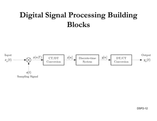
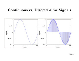
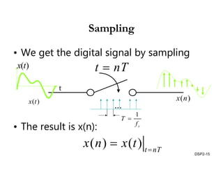
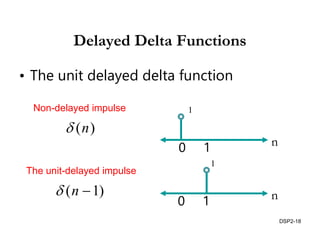
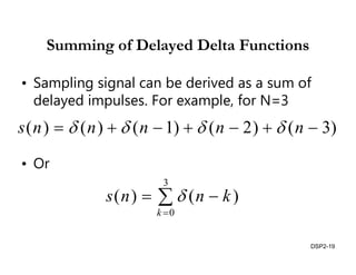
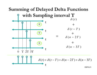
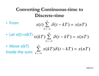
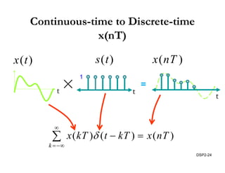
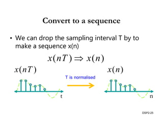
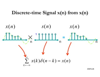
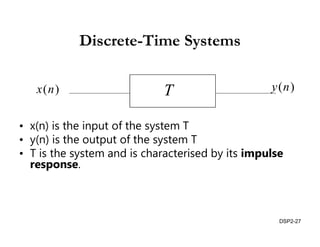
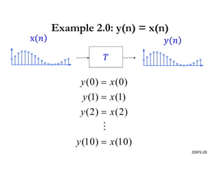
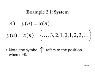
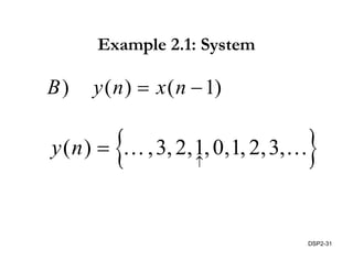
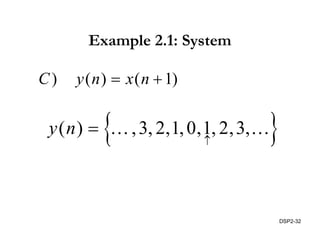
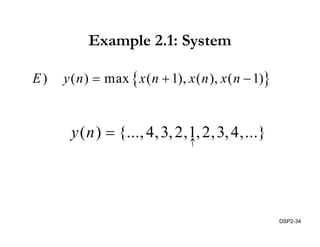
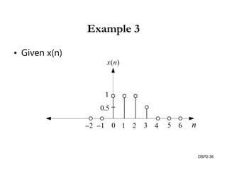
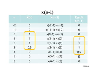
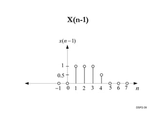
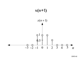
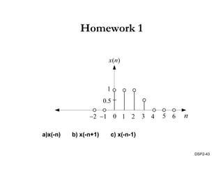
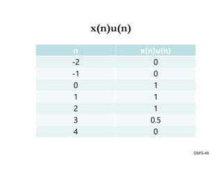
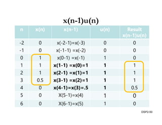
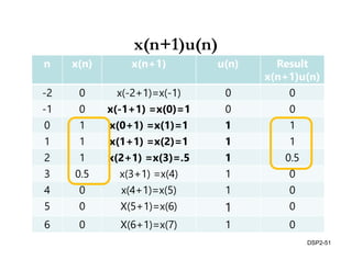
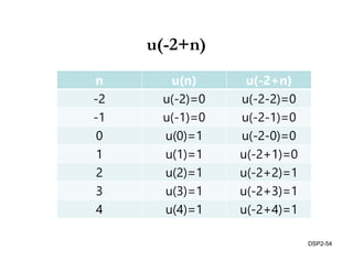
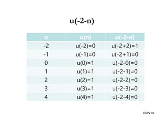
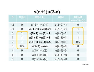
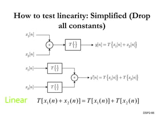
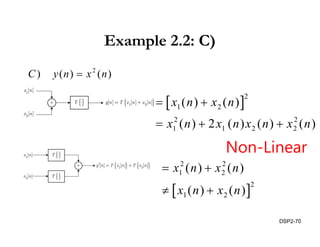
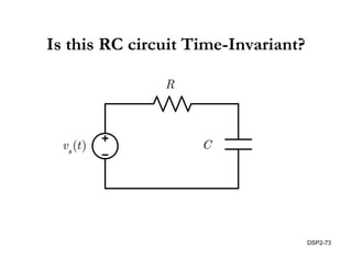
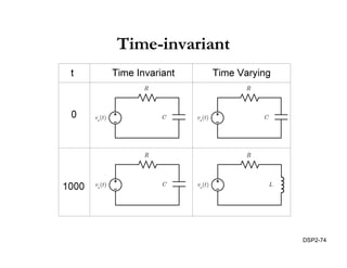
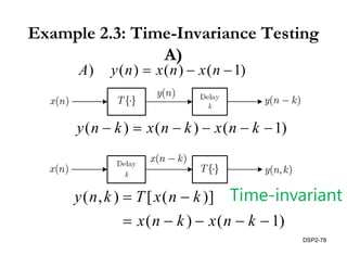
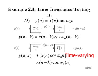
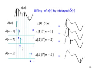
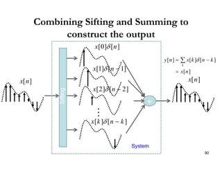
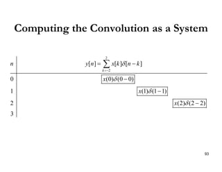
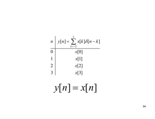
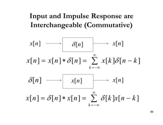
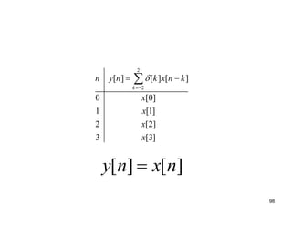
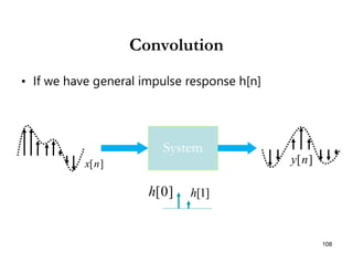
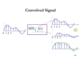
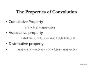
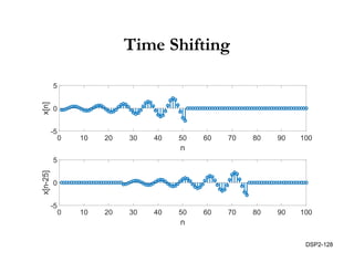
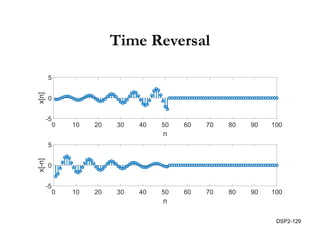
This document discusses discrete-time signals and systems. It defines discrete-time signals as continuous-amplitude signals that are represented by a discrete sequence of values obtained through sampling a continuous-time signal. Linear time-invariant systems are introduced as systems where the output is the input convolved with the system's impulse response. Examples of discrete-time signals and systems are provided to illustrate concepts such as shifting signals by adding or subtracting from the time index n.

1. 2
Discrete-time
Signals and SystemsSignals and Systems
Assoc.Prof.Dr. Peerapol Yuvapoositanon
Mahanakorn Institute of Innovation (MII)
DSP2-1

2. Objectives
• The students understand the concepts of:
– Discrete-time signals and systems
– Linear Time-Invariant Systems
– Convolution– Convolution
DSP2-2

3. Signals
• Signals are the patterns of physical
representation.
• Signals can be represented mathematically as
a function of one or more independenta function of one or more independent
variables, e.g., Time t or Sequence n.
• Signals can be 1-D or 2-D.
3

4. Signals in Electric Circuits
vc(t)
= Signal
i (t)
= Signal
4

5. Signals in Mechanics
F
F
Force
Friction
5

6. Signals in Medicine
• The Electrocardiogram (ECG)
6

7. My 2013 ECG Result
ABNORMAL
(Left Ventricular Hypertrophy)
Normal
7

8. My 2014 ECG Result
ABNORMAL
(Left Ventricular Hypertrophy)
Normal
8

9. My 2019 ECG Result
NORMALNormal
9

10. The Famous Lena Image
10

11. Signal Intensity Values
11

12. Digital Signal Processing Building
Blocks
DSP2-12

13. Continuous vs. Discrete-time Signals
DSP2-13

14. Discrete-Time Continuous Amplitude
• We are only interested in Discrete-Time,
Continuous Amplitude signals.
t
DSP2-14

15. Sampling
• We get the digital signal by sampling
tt
( )x t t nT
• The result is x(n):
( )x t ( )x n
( ) ( ) t nT
x n x t 

...
1
s
T
f

tt
DSP2-15

16. Discrete-time “x(n)” = Sampling “s(n)” x Analogue “x(t)”
Discrete-time signals obtained by
Sampling
tt
( )x t
( )x n
• S(n) is composed of delayed Impulses
nnTT
tt
nn
( )x n( )s n
1
DSP2-16

17. An Impulse is Delta Function
11
( ) ( ) t nT
n t  

• The definition of impulse is
nn00
1, 0
( )
0, 0
n
n
n


 

DSP2-17

18. Delayed Delta Functions
• The unit delayed delta function
11Non-delayed impulse
( )n
nn00
nn
11
The unit-delayed impulse
( 1)n 
( )n
11
00 11
DSP2-18

19. Summing of Delayed Delta Functions
• Sampling signal can be derived as a sum of
delayed impulses. For example, for N=3
( ) ( ) ( 1) ( 2) ( 3)s n n n n n         
• Or
3
0
( ) ( )
k
s n n k

 
DSP2-19

20. Summing of Delayed Delta Functions
( )n
( 1)n 
( 2 )n 
++
++
nn
nn
nn
++
++
== ( 2 )n 
( 3)n 
++
nn
nn
11 22 33
++
==
00
nn
( ) ( 1) ( 2) ( 3)n n n n        
DSP2-20

21. Summing of Delayed Delta Functions
with Sampling interval T
( )t
( )t T 
( 2 )n T 
++
++
tt
tt
tt
++
++
== ( 2 )n T 
( 3 )n T 
++
tt
tt
TT 22TT 33TT
++
==
00
tt
( ) ( ) ( 2 ) ( 3 )t t T n T n T        
DSP2-21

22. Continuous-time to Discrete-time
x(nT)
t
1
( )x t ( )x nT( )s t
t
=
( ) ( ) ( )
k
x t t kT x nT


 
t
tt
t
DSP2-22
=

23. Converting Continuous-time to
Discrete-time
• From
• Let x(t)=x(kT) :
( ) ( ) ( )
k
x t t kT x nT


 
( ) ( ) ( )x kT t kT x nT

 
• Move x(kT)
Inside the sum:
( ) ( ) ( )
k
x kT t kT x nT

 
( ) ( ) ( )
k
x kT t kT x nT


 
DSP2-23

24. Continuous-time to Discrete-time
x(nT)
t
1
( )x t ( )x nT( )s t
t
=t
tt
t
DSP2-24
( ) ( ) ( )
k
x kT t kT x nT


 
=

25. Convert to a sequence
• We can drop the sampling interval T by to
make a sequence x(n)
( ) ( )x nT x n
DSP2-25

nn
( )x n
tt
( )x nT
T is normalised

26. Discrete-time Signal x(n) from x(n)
1
( )x n ( )x n( )s n
=
( ) ( ) ( )
k
x k n k x n


 
nnnn nn
DSP2-26
=

27. Discrete-Time Systems
• x(n) is the input of the system T
T( )x n ( )y n
• x(n) is the input of the system T
• y(n) is the output of the system T
• T is the system and is characterised by its impulse
response.
DSP2-27

28. Example 2.0: y(n) = x(n)
(0) (0)y x(0) (0)
(1) (1)
(2) (2)
(10) (10)
y x
y x
y x
y x





DSP2-28

29. Example 2.1: System 1
• Example 2.2.1
• Determine y(n) when
, 3 3
( )
0, otherwise
n n
x n
   
 

) ( ) ( )A y n x n
 
 
) ( ) ( )
) ( ) ( 1)
) ( ) ( 1)
1
) ( ) ( 1) ( ) ( 1)
3
) ( ) max ( 1), ( ), ( 1)
) ( ) ( )
n
k
A y n x n
B y n x n
C y n x n
D y n x n x n x n
E y n x n x n x n
F y n x k


 
 
    
  
 
DSP2-29

30. Example 2.1: System
) ( ) ( )A y n x n
( ) ( ) ,3,2,1,0,1,2,3,y n x n   
• Note: the symbol refers to the position
when n=0.
DSP2-30
( ) ( ) ,3,2,1,0,1,2,3,y n x n

   


31. Example 2.1: System
) ( ) ( 1)B y n x n 
( ) ,3, 2,1,0,1, 2,3,y n ( ) ,3, 2,1,0,1, 2,3,y n

  
DSP2-31

32. Example 2.1: System
) ( ) ( 1)C y n x n 
( ) ,3, 2,1,0,1, 2,3,y n   ( ) ,3, 2,1,0,1, 2,3,y n

  
DSP2-32

33. Example 2.1: System
 
1
) ( ) ( 1) ( ) ( 1)
3
D y n x n x n x n    
   
1 1 2
0, (0) ( 1) (0) (1) 1 0 1
3 3 3
n y x x x        
3 3 3

2
( ) {...,4,3,2,1, ,1,2,3,4,...}
3
y n


DSP2-33

34. Example 2.1: System
 ) ( ) max ( 1), ( ), ( 1)E y n x n x n x n  
( ) {...,4,3,2,1,2,3,4,...}y n ( ) {...,4,3,2,1,2,3,4,...}y n


DSP2-34

35. Example 2.1 : System
•
• Accumulator
) ( ) ( )
n
k
F y n x k

 
( ) ,3,5,6,6,7,9,12,0,...y n

 
DSP2-35

36. Example 3
• Given x(n)
DSP2-36

37. x(n)
n X(n)
-2 0
-1 0
0 10 1
1 1
2 1
3 0.5
4 0
DSP2-37

38. x(n-1)
n X(n) X(n-1) Result
X(n-1)
-2 0 x(-2-1)=x(-3) 0
-1 0 x(-1-1) =x(-2) 0
0 1 x(0-1) =x(-1) 0
1 1 x(1-1) =x(0) 11 1 x(1-1) =x(0) 1
2 1 x(2-1) =x(1) 1
3 0.5 x(3-1) =x(2) 1
4 0 x(4-1)=x(3) 0.5
5 0 X(5-1)=x(4) 0
6 0 X(6-1)=x(5) 0
DSP2-38

39. X(n-1)
DSP2-39

40. x(n) vs. x(n-1)
DSP2-40

41. x(n+1)
n X(n) X(n+1) Result
X(n+1)
-2 0 x(-2+1)=x(-1) 0
-1 0 x(-1+1) =x(0) 1
0 1 x(0+1) =x(1) 1
1 1 x(1+1) =x(2) 11 1 x(1+1) =x(2) 1
2 1 x(2+1) =x(3) 0.5
3 0.5 x(3+1) =x(4) 0
4 0 x(4+1)=x(5) 0
5 0 X(5+1)=x(6) 0
6 0 X(6+1)=x(7) 0
DSP2-41

42. x(n+1)
DSP2-42

43. Homework 1
a)x(-n) b) x(-n+1) c) x(-n-1)
DSP2-43

44. Unit Step Sequence
1, 0
( )
0, 0
n
u n
n

 

DSP2-44

45. Relationship between the unit step
function and the Delta function
• Define u(n)
( ) ( ) ( 1) ( 2) ( 3)
( )
u n n n n n
n k
   


       
 

Or
0
( )
k
n k

 
( ) ( )
n
k
u n k

 
DSP2-45

46. Example 4
• Let x(n) be
• Determine ) ( ) ( )
) ( 1) ( )
) ( 1) (2 )
) ( 1) ( 1 )
a x n u n
b x n u n
c x n u n
d x n u n

 
   
DSP2-46

47. x(n)
n x(n)
-2 0
-1 0
0 10 1
1 1
2 1
3 0.5
4 0
DSP2-47

48. u(n)
n u(n)
-2 u(-2)=0
-1 u(-1)=0
0 u(0)=1
DSP2-48
0 u(0)=1
1 u(1)=1
2 u(2)=1
3 u(3)=1
4 u(4)=1

49. x(n)u(n)
n x(n)u(n)
-2 0
-1 0
0 1
DSP2-49
0 1
1 1
2 1
3 0.5
4 0

50. x(n-1)u(n)
n x(n) x(n-1) u(n) Result
x(n-1)u(n)
-2 0 x(-2-1)=x(-3) 0 0
-1 0 x(-1-1) =x(-2) 0 0
0 1 x(0-1) =x(-1) 1 0
1 1 x(1-1) =x(0)=1 1 11 1 x(1-1) =x(0)=1 1 1
2 1 x(2-1) =x(1)=1 1 1
3 0.5 x(3-1) =x(2)=1 1 1
4 0 x(4-1)=x(3)=.5 1 0.5
5 0 X(5-1)=x(4) 1 0
6 0 X(6-1)=x(5) 1 0
DSP2-50

51. x(n+1)u(n)
n x(n) x(n+1) u(n) Result
x(n+1)u(n)
-2 0 x(-2+1)=x(-1) 0 0
-1 0 x(-1+1) =x(0)=1 0 0
0 1 x(0+1) =x(1)=1 1 1
1 1 x(1+1) =x(2)=1 1 11 1 x(1+1) =x(2)=1 1 1
2 1 x(2+1) =x(3)=.5 1 0.5
3 0.5 x(3+1) =x(4) 1 0
4 0 x(4+1)=x(5) 1 0
5 0 X(5+1)=x(6) 1 0
6 0 X(6+1)=x(7) 1 0
DSP2-51

52. u(2-n)
n u(n) u(2-n)
-2 u(-2)=0 u(2+2)=1
-1 u(-1)=0 u(2+1)=1
0 u(0)=1 u(2-0)=1
DSP2-52
0 u(0)=1 u(2-0)=1
1 u(1)=1 u(2-1)=1
2 u(2)=1 u(2-2)=1
3 u(3)=1 u(2-3)=0
4 u(4)=1 u(2-4)=0

53. u(2+n)
n u(n) u(2+n)
-2 u(-2)=0 u(2-2)=1
-1 u(-1)=0 u(2-1)=1
0 u(0)=1 u(2-0)=1
DSP2-53
0 u(0)=1 u(2-0)=1
1 u(1)=1 u(2+1)=1
2 u(2)=1 u(2+2)=1
3 u(3)=1 u(2+3)=1
4 u(4)=1 u(2+4)=1

54. u(-2+n)
n u(n) u(-2+n)
-2 u(-2)=0 u(-2-2)=0
-1 u(-1)=0 u(-2-1)=0
0 u(0)=1 u(-2-0)=0
DSP2-54
0 u(0)=1 u(-2-0)=0
1 u(1)=1 u(-2+1)=0
2 u(2)=1 u(-2+2)=1
3 u(3)=1 u(-2+3)=1
4 u(4)=1 u(-2+4)=1

55. u(-2-n)
n u(n) u(-2-n)
-2 u(-2)=0 u(-2+2)=1
-1 u(-1)=0 u(-2+1)=0
0 u(0)=1 u(-2-0)=0
DSP2-55
0 u(0)=1 u(-2-0)=0
1 u(1)=1 u(-2-1)=0
2 u(2)=1 u(-2-2)=0
3 u(3)=1 u(-2-3)=0
4 u(4)=1 u(-2-4)=0

56. x(n+1)u(2-n)
n x(n) x(n+1) u(n) Result
x(n+1)u(n)
-2 0 x(-2+1)=x(-1) u(2+2)=1 0
-1 0 x(-1+1) =x(0)=1 u(2+1)=1 1
0 1 x(0+1) =x(1)=1 u(2-0)=1 1
1 1 x(1+1) =x(2)=1 u(2-1)=1 11 1 x(1+1) =x(2)=1 u(2-1)=1 1
2 1 x(2+1) =x(3)=.5 u(2-2)=1 0.5
3 0.5 x(3+1) =x(4) u(2-3)=0 0
4 0 x(4+1)=x(5) u(2-4)=0 0
5 0 X(5+1)=x(6) u(2+5)=0 0
6 0 X(6+1)=x(7) u(2+6)=0 0
DSP2-56

57. Systems
• A system is any process that produces an
output signal in response to an input signal.
• Systems are can also be represented
mathematically as a function of one or moremathematically as a function of one or more
independent variables, e.g., Time t or
Sequence n.
57

58. An Electric Circuit System
• System of a simple RC circuit.
vc(t)
=Signal
System
vc(t)
= Signal
58

59. Model of Simple RC Circuit
• Using Kirchoff’s Voltage Law (KVL)
( ) ( ) ( )
( ) ( ) ( )
R c s
c s
v t v t v t
Ri t v t v t
 
 ( ) ( ) ( )
( ( )) ( ) ( )
c s
c c s
Ri t v t v t
d
R C v t v t v t
dt
 
 
1 1
( ) ( ) ( )c c s
d
v t v t v t
dt RC RC
 
59

60. Linear Constant-Coefficient Differential
Equation (LCCDE)
• Linear Constant-Coefficient Differential
Equation (LCCDE)
( ) ( )k kN M
k kk k
d y t d x t
a b
dt dt
 
• For 1st order:
• or: 1 1
( ) ( ) ( )c c s
d
v t v t v t
dt RC RC
 
0 0
k kk k
k kdt dt 
 
1 0 0( ) ( ) ( )
d
a y t a y t b x t
dt
 
60

61. System Model of A Car
Zhou, Hui & Qiu, Yi. (2015). A simple mathematical model of a vehicle with seat and occupant for studying the effect of vehicle dynamic parameters on ride comfort.
61

62. System Model of A Heart
Yalcinkaya, Fikret & Kizilkaplan, Ertem & Erbas, Ali. (2013). Mathematical modelling of human heart as a hydroelectromechanical system. ELECO 2013 - 8th International Conference on Electrical
and Electronics Engineering. 362-366. 10.1109/ELECO.2013.6713862.
62

63. Linear Time-invariant (LTI) Systems
• A discrete-time system T[ ] can either be
– Linear or Non-linear
– Time-invariant or Time-varying
• We prefer systems that are Linear and Time-
invariant.
( )x n
( ) [ ( )]y n T x n
T
DSP2-63

64. Linear Systems
• For a system to be linear,
T1 1 2 2( ) ( ) ( )x n a x n a x n 
1 1 2 2
1 1 2 2
( ) ( ) ( )
[ ( )] [ ( )]
y n a y n a y n
a T x n a T x n
 
 
DSP2-64
1 1 2 2 1 1 2 2[ ( ) ( )] [ ( )] [ ( )]T a x n a x n a T x n a T x n  
T1 1 2 2( ) ( ) ( )x n a x n a x n 

65. How to test linearity: Full Test
DSP2-65
1 1 2 2 1 1 2 2[ ( ) ( )] [ ( )] [ ( )]T a x n a x n a T x n a T x n  Linear

66. How to test linearity: Simplified (Drop
all constants)
DSP2-66
Linear 1 2 1 2[ ( ) ( )] [ ( )] [ ( )]T x n x n T x n T x n  

67. Example 2.2
• Determine whether the systems are linear or
non-linear.
2
) ( ) ( )
) ( ) ( )
A y n nx n
B y n x n

 2
2
( )
) ( ) ( )
) ( ) ( )
) ( ) ( )
) ( ) x n
B y n x n
C y n x n
D y n Ax n B
E y n e


 

DSP2-67

68. Example 2.2: A)
) ( ) ( )A y n nx n
1 2[ ( ) ( )]
( ) ( )
n x n x n
nx n nx n
 
 
1 2( ) ( )nx n nx n 
DSP2-68
1 2( ) ( )nx n nx n 
Linear

69. Example 2.2: B)
2
) ( ) ( )B y n x n
2 2
1 2( ) ( )x n x n 
DSP2-69
2 2
1 2( ) ( )x n x n 
Linear

70. Example 2.2: C)
2
) ( ) ( )C y n x n
 2
1 2
2 2
( ) ( )
( ) 2 ( ) ( ) ( )
x n x n
x n x n x n x n
 
  
 
2 2
1 2
2
1 2
( ) ( )
( ) ( )
x n x n
x n x n
 
 
DSP2-70
2 2
1 1 2 2( ) 2 ( ) ( ) ( )x n x n x n x n  
Non-Linear

71. Example 2.2: D)
) ( ) ( )D y n Ax n B 
 
1 2
1 2
[ ( ) ( )]
( ) ( )
T x n x n
A x n x n B
 
   1 2( ) ( )A x n x n B  
DSP2-71
1 2[ ( ) ] [ ( ) ]Ax n B Ax n B   
Non-Linear
 1 2( ) ( )A x n x n B  

72. Example 2.2: E)
( )
) ( ) x n
E y n e
1 2( ) ( )x n x n
e 

Non-Linear
DSP2-72
1 2( ) ( )x n x n
e e 
Non-Linear
1 2( ) ( )x n x n
e 


73. Is this RC circuit Time-Invariant?
DSP2-73

74. Time-invariant
DSP2-74

75. Time-Invariant Test
(Continuous-Time Systems)
• Tested by comparing the following systems.
DSP2-75
0 0( , ) ( )y t t y t t Time-Invariant

76. Time-Invariant Test
(Discrete-Time Systems)
DSP2-76
( , ) ( )y n k y n k Time-Invariant

77. Example 2.3: Time-Invariance Testing
• Determine whether the following systems are
Time-invariant or Time-varying
) ( ) ( ) ( 1)A y n x n x n  
0
) ( ) ( )
) ( ) ( )
) ( ) ( ) cos
B y n nx n
C y n x n
D y n x n n

 

DSP2-77

78. Example 2.3: Time-Invariance Testing
A)
) ( ) ( ) ( 1)A y n x n x n  
( ) ( ) ( 1)y n k x n k x n k     
( , ) [ ( )]
( ) ( 1)
y n k T x n k
x n k x n k
 
    
( ) ( ) ( 1)y n k x n k x n k     
DSP2-78
Time-invariant

79. Example 2.3: Time-Invariance Testing
B)
) ( ) ( )B y n nx n
( ) ( ) ( )y n k n k x n k   
( , ) [ ( )]
( )
y n k T x n k
nx n k
 
 
( ) ( ) ( )y n k n k x n k   
DSP2-79
Time-varying

80. Example 2.3: Time-Invariance Testing
C)
( ) ( ( )) ( )y n k x n k x n k      
) ( ) ( )C y n x n 
( , ) [ ( )]
( )
y n k T x n k
x n k
  
  
( ) ( ( )) ( )y n k x n k x n k      
DSP2-80
Time-varying

81. Example 2.3: Time-Invariance Testing
D)
0( ) ( ) cos ( )y n k x n k n k   
0) ( ) ( ) cosD y n x n n
0
0
( , ) [ ( ) cos ]
( ) cos ( )
y n k T x n n
x n k n



 
0( ) ( ) cos ( )y n k x n k n k   
DSP2-81
Time-varying

82. Why is the LTI Systems so Important?
• The LTI property allows us to analyse the
characteristics of the system.
• Above all, with this LTI property, the system
can be used to find the relationship betweencan be used to find the relationship between
the input, the impulse response and the
output of the system.
• We are talking about the Convolution.
DSP2-82

83. h[n] has multiple components
• Consider the DT case. (Easier than CT!)
• h[n] has multiple components.
[ ]x n [ ]y n
SystemSystem
[ ]h n =Impulse Response
0 1
1 0.8
83

84. h[n] has only one component
• Now, let h[n] be a signal with only one
component.
• We call this type of signal as a unit impulse.
[ ]x n [ ] [ ]y n x n
SystemSystem
0
1 [ ]h n =Impulse Response
84

85. An Impulse is Delta Function
• The definition of unit impulse is
1, 0
[ ]
0, 0
n
n
n


 
0, 0n 
0 n
1
85

86. Delayed Delta Functions
• The unit delayed delta function
Unit impulse
[ ]n
1
The unit-delayed impulse
[ 1]n 
[ ]n
0 n
0 n
1
1
86

87. Multiple Delayed [n]
The unit-delayed impulse
[ 1]n 
0 n
1
1
The 2-delayed impulse 1
[ 2]n 
0 n1
The k-delayed impulse
[ ]n k 
0 n
1
1
2
2 k
87
 

88. [ ]x n
n
1
0
1 n
1
1
=
=
[0] [ ]x n
[1] [ 1]x n 
[ ]n
[ 1]n 
Sifting of x[n] by (delayed)[n]
nk
1 n
2 n
1
1
=
=
[2] [ 2]x n 
[ ] [ ]x k n k 
[ 2]n 
[ ]n k 
88
 

89. [0] [ ]x n
[1] [ 1]x n 
Summation of Each Signal
[2] [ 2]x n 
[ ] [ ]x k n k 
+
[ ]x n
[ ] [ ] [ ] [ ]
k
y n x k n k x n  
89


90. Combining Sifting and Summing to
construct the output
[0] [ ]x n
[1] [ 1]x n 
[2] [ 2]x n 
[ ]x n
[ ] [ ] [ ]
[ ]
k
y n x k n k
x n
 


[ ]x n
[2] [ 2]x n 
[ ] [ ]x k n k 
+
System
90

Sifting

91. Construction of Signal From Sifted
Components
• Construction of Signal From Sifted Components
is then written as
[ ] [ ] [ ]
k
x n x k n k


 
• Since this is operation of x[n] and [n], we write
• This is called the “Convolution equation” between
x[n] and [n].
k 
[ ] [ ] [ ]x n x n n 
91

92. System defined by [n]
[ ] [ ]y n x n[ ]n( )x n
[ ] [ ] [ ] [ ] [ ]
k
x n x k n k x n n 


   
92

93. Computing the Convolution as a System
2
2
[ ] [ ] [ ]
0 ( 2) (0 2) ( 1) (0 1) (0) (0 0) (1) (0 1) (2) (0 2)
k
n y n x k n k
x x x x x

    

 
          

1 ( 2) (1 2) ( 1) (1 1) (0) (1 0) (1) (1 1) (2) (1 2)
2 ( 2) (2 2) ( 1) (2 1) (0) (2 0) (1) (2 1) (2) (2 2)
3 ( 2)
x x x x x
x x x x x
x
    
    

          
          
 (3 2) ( 1) (3 1) (0) (3 0) (1) (3 1) (2) (3 2)x x x x            
93

94. 2
2
[ ] [ ] [ ]
0 [0]
1 [1]
k
n y n x k n k
x
x


 
1 [1]
2 [2]
3 [3]
x
x
x
[ ] [ ]y n x n
94

95. Finding Impulse Response
• If delta function is input, output will be h[n]
[ ] [ ]y n h n[ ]n [ ]h n
[ ] [ ] [ ] [ ] [ ]
k
h n n h n k h n k 


   
h[n] = Impulse
Response
95

96. Input and Impulse Response are
Interchangeable (Commutative)
[ ] [ ] [ ] [ ] [ ]x n x n n x k n k 

   
[ ]x n [ ]n [ ]x n
[ ]x n[ ]n [ ]x n
[ ] [ ] [ ] [ ] [ ]
k
x n n x n k x n k 


   
96
[ ] [ ] [ ] [ ] [ ]
k
x n x n n x k n k 

   

97. Example
• Determine
2
2
[ ] [ ] [ ]
k
n y n k x n k

 
2
2
[ ] [ ] [ ]
k
y n k x n k

 
2
0 ( 2) (0 2) ( 1) (0 1) (0) (0 0) (1) (0 1) (2) (0 2)
1 ( 2) (1 2) ( 1) (1 1) (0) (1 0) (1) (1 1) (2) (1 2)
2 ( 2) (2 2) ( 1) (2 1) (0) (2 0) (1) (2 1) (2) (2 2)
3 ( 2)
k
x x x x x
x x x x x
x x x x x
x
    
    
    


          
          
          
 (3 2) ( 1) (3 1) (0) (3 0) (1) (3 1) (2) (3 2)x x x x            
97

98. 2
2
[ ] [ ] [ ]
0 [0]
1 [1]
k
n y n k x n k
x
x


 
1 [1]
2 [2]
3 [3]
x
x
x
[ ] [ ]y n x n
98

99. Comparison between the two
convolutions
DSP2-99

100. SystemSystem
System with Delayed Delta function
[ ] [ 1]y n x n 
SystemSystem
[ ] [ 1]h n n 
[ ] [ 1]h n n 
[ ]x n
100

101. 2
2
[ ] [ 1] [ ]
0 ( 3) (2) ( 2) (1) ( 1) (0) (0) ( 1) (1) ( 2)
1 ( 3) (3) ( 2) (2) ( 1) (1) (0) (0) (1) ( 1)
k
n y n k x n k
x x x x x
x x x x x

    
    

  
        
       

2
2
( ) ( ) ( )
k
y n h k x n k

 
1 ( 3) (3) ( 2) (2) ( 1) (1) (0) (0) (1) ( 1)
2 ( 3) (4) ( 2) (3) ( 1) (2) (0) (1) (1) (0)
3 ( 3) (5) ( 2) (4) ( 1) (3
x x x x x
x x x x x
x x x
    
    
  
       
      
     ) (0) (2) (1) (1)x x  
1, 0
[ ]
0, 0
n
n
n


 

101

102. 2
2
[ ] [ 1] [ ]
0 [ 1]
1 [0]
k
n y n k x n k
x
x


  


1 [0]
2 [1]
3 [2]
x
x
x
[ ] [ 1]y n x n 
102

103. Delayed Signal
nn
( ) ( 1)y n x n 
11 2200 33
nn11 2200 33
103

104. SystemSystem
System with and without
Delayed Delta functions
•
( ) ( 1)y n x n 
SystemSystem
( ) ( ) ( 1)h n n n   
[ ] [ ] [ 1]h n n n   
( )x n
104

105. Example
• Let
• Find
[ ] [ ] [ 1]h n n n   
• Find
• For n=0,...,3
2
2
[ ] [ ] [ ]
k
y n h k x n k

 
105

106. 2
2
( ) [ ( ) ( 1)] ( )
( 2) (2) ( 1) (1) (0) (0) (1) ( 1) (2) ( 2)
0
( 3) (2) ( 2) (1) ( 1) (0) (0) ( 1) (1) ( 2)
( 2) (3) ( 1) (2) (0) (1) (1) (0) (2) (1)
k
n y n k k x n k
x x x x x
x x x x x
x x x x x
 
    
    
    

   
        
        
      

2
2
( ) ( ) ( )
k
y n h k x n k

 
( 2) (3) ( 1) (2) (0) (1) (1) (0) (2) (1)
1
( 3) (3) ( 2) (2) (
x x x x x
x x
    
  
      
    1) (1) (0) (0) (1) ( 1)
( 2) (4) ( 1) (3) (0) (2) (1) (1) (2) (0)
2
( 3) (4) ( 2) (3) ( 1) (2) (0) (1) (1) (0)
( 2) (5) ( 1) (4) (0) (3) (1) (2) (2) (1)
3
( 3) (5) ( 2) (4) ( 1) (3)
x x x
x x x x x
x x x x x
x x x x x
x x x
 
    
    
    
   
   
      
      
      
      (0) (2) (1) (1)x x
106

107. 2
2
( ) ( ) ( )
0 (0) ( 1)
1 (1) (0)
k
n y n k x n k
x x
x x


 
 


1 (1) (0)
2 (2) (1)
3 (3) (2)
x x
x x
x x



[ ] [ ] [ 1]y n x n x n  
107

108. Convolution
• If we have general impulse response h[n]
[ ]x n [ ]y n
SystemSystem
[0]h [1]h
108

109. Convolved Signal
++
11 2200 33
[0]h [1]h
++
11 2200 33
11 2200 33
109

110. Example
• Now if the impulse response is consisted of a
scaled unit delayed
( ) {1,0.8}h n


• Or h(0) =1 and h(1) =0.8
• This means we can write h(n) as
DSP2-110
( ) ( ) 0.8 ( 1)h n n n   
( ) {1,0.8}h n



111. Convolution of x(n) and h(n) = {1,0.8}
( ) ?y n h(n)h(n) ( ) ?y n 
(0)h (1)h
DSP2-111
0 1
h(n)h(n)
( ) ( ) 0.8 ( 1)h n n n   
( )x n

112. Convolved Signal
++
11 2200 33
(0)h (1)h
++
11 2200 33
11 2200 33
DSP2-112

113. ( 2) (2) ( 1) (1) (0) (0) (1) ( 1) (2) ( 2)x x x x x             
Calculate Convolution at n=0
n =0 and let k=-2,-1,0,1,2
2 2
2 2
(0) ( ) (0 ) 0.8 ( 1) (0 )
k k
y k x k k x k 
 
     
( 2) (2) ( 1) (1) (0) (0) (1) ( 1) (2) ( 2)
0.8[ ( 3) (2) ( 2) (1) ( 1) (0) (0) ( 1) (1) ( 2)]
x x x x x
x x x x x
    
    
         
        
DSP2-113
(0) 0.8 ( 1)x x  

114. ( 2) (3) ( 1) (2) (0) (1) (1) (0) (2) (1)x x x x x           
Calculate Convolution at n=1
n =1 and let k=-2,-1,0,1,2
2 2
2 2
(1) ( ) (1 ) 0.8 ( 1) (1 )
k k
y k x k k x k 
 
     
( 2) (3) ( 1) (2) (0) (1) (1) (0) (2) (1)
0.8 ( 3) (3) ( 2) (2) ( 1) (1) (0) (0) (1) ( 1)
x x x x x
x x x x x
    
    
       
         
DSP2-114
(1) 0.8 (0)x x 

115. ( 2) (4) ( 1) (3) (0) (2) (1) (1) (2) (0)x x x x x           
Calculate Convolution at n=2
n =2 and let k=-2,-1,0,1,2
2 2
2 2
(2) ( ) (2 ) 0.8 ( 1) (2 )
k k
y k x k k x k 
 
     
( 2) (4) ( 1) (3) (0) (2) (1) (1) (2) (0)
0.8 ( 3) (4) ( 2) (3) ( 1) (2) (0) (1) (1) (0)
x x x x x
x x x x x
    
    
       
        
DSP2-115
(2) 0.8 (1)x x 

116. ( 2) (5) ( 1) (4) (0) (3) (1) (2) (2) (1)x x x x x           
Calculate Convolution at n=3
n =3 and let k=-2,-1,0,1,2
2 2
2 2
(3) ( ) (3 ) 0.8 ( 1) (3 )
k k
y k x k k x k 
 
     
( 2) (5) ( 1) (4) (0) (3) (1) (2) (2) (1)
0.8 ( 3) (5) ( 2) (4) ( 1) (3) (0) (2) (1) (1)
x x x x x
x x x x x
    
    
       
        
DSP2-116
(3) 0.8 (2)x x 

117. ( )
0 (0) 0.8 ( 1)
1 (1) 0.8 (0)
2 (2) 0.8 (1)
n y n
x x
x x
x x
 

2 (2) 0.8 (1)
3 (3) 0.8 (2)
x x
x x


( ) ( ) 0.8 ( 1)y n x n x n  
DSP2-117

118. Example 1: Convolution
• Determine the convolution results of
y(n)=x(n)*h(n) for n=0,…,3 where
( ) {3,2}h n


and x(n) and h(n) are zero for other values of n.
( ) {3,2}h n


( ) {5,4}x n


DSP2-118

119. Solution
• From
• If h(n) and x(n) is zero when 0< n and n> 1,
( ) ( ) ( )
k
y n h k x n k


 
• If h(n) and x(n) is zero when 0< n and n> 1,
then we calculate convolution only for h(0) =0
and 1.
• Note that, like n, k is just an index for the sum.
1
0
( ) ( ) ( )
k
y n h k x n k

 
DSP2-119

120. 3 ( 2) (2) ( 1) (1) (0) (0) (1) ( 1) (2) ( 2)x x x x x              
Calculate Convolution at n=0
n =0 and let k=-2,-1,0,1,2
2 2
2 2
(0) 3 ( ) (0 ) 2 ( 1) (0 )
k k
y k x k k x k 
 
     
3 ( 2) (2) ( 1) (1) (0) (0) (1) ( 1) (2) ( 2)
2[ ( 3) (2) ( 2) (1) ( 1) (0) (0) ( 1) (1) ( 2)]
x x x x x
x x x x x
    
    
           
        
DSP2-120
3 (0) 2 ( 1)x x  
3 5 2 0 15    

121. 3 ( 2) (3) ( 1) (2) (0) (1) (1) (0) (2) (1)x x x x x            
Calculate Convolution at n=1
n =1 and let k=-2,-1,0,1,2
2 2
2 2
(1) 3 ( ) (1 ) 2 ( 1) (1 )
k k
y k x k k x k 
 
     
3 ( 2) (3) ( 1) (2) (0) (1) (1) (0) (2) (1)
2 ( 3) (3) ( 2) (2) ( 1) (1) (0) (0) (1) ( 1)
x x x x x
x x x x x
    
    
         
         
DSP2-121
3 (1) 2 (0)x x 
3 4 2 5 22    

122. 3 ( 2) (4) ( 1) (3) (0) (2) (1) (1) (2) (0)x x x x x            
Calculate Convolution at n=2
n =2 and let k=-2,-1,0,1,2
2 2
2 2
(2) 3 ( ) (2 ) 3 ( 1) (2 )
k k
y k x k k x k 
 
     
3 ( 2) (4) ( 1) (3) (0) (2) (1) (1) (2) (0)
2 ( 3) (4) ( 2) (3) ( 1) (2) (0) (1) (1) (0)
x x x x x
x x x x x
    
    
         
        
DSP2-122
3 (2) 2 (1)x x 
3 0 2 4 8    

123. 3 ( 2) (5) ( 1) (4) (0) (3) (1) (2) (2) (1)x x x x x            
Calculate Convolution at n=3
n =3 and let k=-2,-1,0,1,2
2 2
2 2
(3) 3 ( ) (3 ) 2 ( 1) (3 )
k k
y k x k k x k 
 
     
3 ( 2) (5) ( 1) (4) (0) (3) (1) (2) (2) (1)
2 ( 3) (5) ( 2) (4) ( 1) (3) (0) (2) (1) (1)
x x x x x
x x x x x
    
    
         
        
DSP2-123
3 (3) 2 (2)x x 
3 0 2 0 0    

124. ( )
0 3 (0) 2 ( 1)
1 3 (1) 2 (0)
2 3 (2) 3 (1)
n y n
x x
x x
x x
 

2 3 (2) 3 (1)
3 3 (3) 2 (2)
x x
x x


( ) 3 ( ) 2 ( 1)y n x n x n  
DSP2-124

125. Homework 2
• Determine in details the convolution results of
y(n)=x(n)*h(n) for n=-1,…,3 where
( ) [1, 2,3]x n 
• and x(n) and h(n) are zero for other values of
n.
( ) [1, 2,3]x n


( ) [1,1,1]h n


DSP2-125

126. Answer
( ) ( ) ( ) ( ) ( )
( ) ( ) ( ) ( )
y n h n x n x n h n
h k x n k x k h n k
 
   
    ( ) ( ) ( ) ( )
[1,3,6,5,3]
k k
h k x n k x k h n k
 

   

 
DSP2-126

127. The Properties of Convolution
• Cumulative Property
• Associative property
( ) ( ) ( ) ( )x n h n h n x n  
• Distributive property
•
1 2 1 2{ ( ) ( )} ( ) ( ) { ( ) ( )}x n h n h n x n h n h n    
1 2 1 2( ) { ( ) ( )} ( ) ( ) ( ) ( )x n h n h n x n h n x n h n     
DSP2-127

128. Time Shifting
0 10 20 30 40 50 60 70 80 90 100
x[n]
-5
0
5
n
0 10 20 30 40 50 60 70 80 90 100
n
0 10 20 30 40 50 60 70 80 90 100
x[n-25]
-5
0
5
DSP2-128

129. Time Reversal
0 10 20 30 40 50 60 70 80 90 100
x[n]
-5
0
5
n
0 10 20 30 40 50 60 70 80 90 100
n
0 10 20 30 40 50 60 70 80 90 100
x[-n]
-5
0
5
DSP2-129