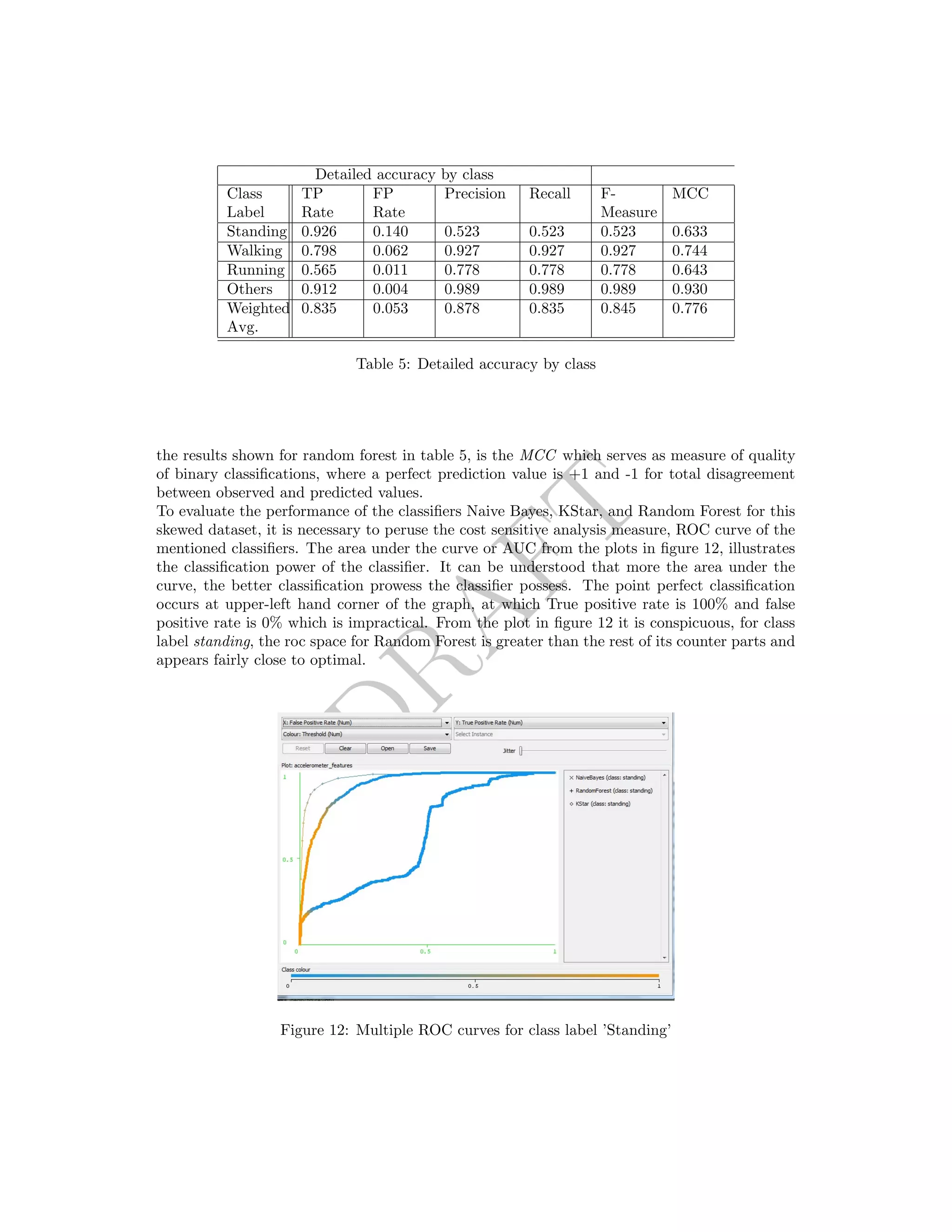
This document describes a framework for classifying human activities like standing, walking, and running using data from an accelerometer sensor on a smartphone. It discusses collecting raw sensor data, preprocessing the data through smoothing and feature extraction, training classifiers on extracted features, and classifying new data in real-time. Random forest classification achieved 83.49% accuracy on this activity recognition task using accelerometer data from an Android application.

1. DRAFT
Activity recognition from accelerometer data
Raghunandan Palakodety2∗
Informatik IV, Universit¨at Bonn, Germany
s6rapala@uni-bonn.de
Abstract
In the last decade, there has been an ever increasing research activity on human activity
recognition. The research in classifying tasks ranging from simple to most complex such
as eye tracking, introduced many architectures using inertial sensors along with on-board
motion sensors in a smartphone. To understand more about the activities, analyzing the
data that emanate from various sensors can be conducive to formulate mathematical mod-
els for classifying independent data. For classifying selected activities such as standing,
walking, running and idle, we have chosen accelerometer sensor to formulate a model for
those activities. To achieve the mentioned tasks, we have developed an application for
classifying above activities in real-time. The application uses accelerometer data to con-
struct real-time instances and uses machine learning algorithms to train various classifiers,
later the classifiers’ performances are compared. Thus, with Random Forest classifier we
reach a performance of 83.4901%.
1 Introduction
This paper describes a prevalent approach for classifying selected activities such as standing,
walking, running and idle using a gamut of algorithms, in particular ensemble learning method.
An application was developed on Android OS platform to achieve the above mentioned task of
classification. The architecture for the application includes collecting raw data from accelerome-
ter sensor which subsequently undergoes three phases namely, pre-processing, feature selection,
feature extraction. A mathematical model is then fitted with the training data obtained from
the above mentioned phases. Later, the application classifies data obtained, also known as
test data in the classification phase. The evaluation phase of the architecture, analyzes the
performance of classifiers by their accuracies and in particular using confusion matrices.
This paper is structured into sections in which section 1.1 elucidates selected research activities
in human activity recognition domain and section 2 describes the general idea and the pro-
posed architecture for this lab task. Section3 and 4 explains the reasons behind pre-processing
and smoothing. In section5 and section6, we describe the method of extracting features from
raw data and constructing feature vectors respectively. In Section7, we describe the necessity
and use of cross-validation technique followed by confusion matrices. Section8 contains the
description and pseudo code of a particular classifier we use for classification which is dealt
subsequently in section9. In section10, we evaluate the efficiency of a single Classification and
Regression Tree or CART decision tree as compared to a procedure known as bagging. The
results of this lab work are illustrated in section11 in which, detailed accuracies of activities
classified by various classifiers are discussed using various estimators. The paper ends with a
section12 in which we present approaches for augmenting the existing classification rates.
∗Dr. Welke and chair for reviewing the paper
1

2. DRAFT
1.1 Related Work
Many commercial applications for user activity recognition tasks have been developed and are
available for various mobile platforms. Fitness applications such as PaceDJ analyzes the pace
of the the jogger and prompts a song of particular beats per minute to be played [7]. Face-
Lock enables user to unlock the phone and applications using one of the concepts of machine
learning. Apart from these commercial applications which are available on various applica-
tion delivery systems, research on potential participatory and opportunistic applications are
underway. Visage, a face interpretation engine for smartphone applications lets users to drive
applications based on their facial responses, comes under a new class of face-aware applications
for smartphones. The modus operandi of this engine fuses data streams [21] from the handset’s
front camera and built in motion sensors to deduce the user’s 3D head poses (through pitch,
roll, yaw of user’s head with respect to the phone co-ordinate system) and visage expressions.
Ongoing research at OPPORTUNITY at ETH Z¨urich IFE -Wearable computing, is focused on
developing mobile systems to recognize human activity and user context with dynamically vary-
ing sensor setups, using goal oriented, cooperative sensing [13]. Such systems are also known
as opportunistic, since they take advantage of sensing modalities that are available instead of
leveraging the user to deploy specific, application dependent sensor systems.
Many such activity recognition tasks are implemented independently with a gamut of architec-
tures and designs. To date, there is no single exhaustive tutorial on a framework that present
the design, implementation, and evaluation of Human Activity Recognition systems. The pa-
per [5], introduces a concept of activity recognition chain, also known as ARC, as a general
purpose framework for designing and evaluating activity recognition systems. The framework
comprises components for data acquisition, pre-processing, data segmentation, decision fusion,
and performance evaluation. At the end of the paper by Mulling et al [5], a problem setting
of recognizing different hand gestures using inertial sensors attached to lower and upper arm is
presented and the implementation of each component in ARC framework for the recognition
problem is discussed. It is demonstrated how different design decisions and their impact on
overall recognition performance fare.
Another article [11], introduced a comprehensive approach for context aware applications that
utilizes the multi-modal sensors in smartphone handsets. Their proposed system not only rec-
ognizes different kinds of contexts with high accuracy, but it is also able to optimize the power
consumption of sensors that can be activated and deactivated at appropriate times. Further
more, a novel feature selection algorithm is proposed for accelerometer classification module
of their architecture. In essence, their feature selection algorithm is based on measuring the
quality of a feature using two estimators, relevancy (or classification power) and redundancy
(or similarity between two selected features) [11]. Recently, another sophisticated solution was
proposed by [9] to find the location of the phone in order to support context-aware applications.
The solution gives 97% accuracy in detecting the position of the phone as well as being able to
correlate with the type of location the user is in. Their implementation includes features such
as extraction of Mel Frequency Cepstral Coefficients or MFCC, Delta Mel Frequency Cepstral
or DMFCC and Band Energy features.
2 Concept
2.1 Background
The android platform supports three broad categories of sensors which are motion sensors,
environment sensors and position sensors. Of these, motion sensors category are extremely

3. DRAFT
conducive for monitoring device movement, such as tilt, shake rotation or swing. This category
includes accelerometers, gravity sensors, gyroscopes and rotational vector sensors. Two of the
these sensors are always hardware based (the accelerometer and gyroscope), and the rest can be
either hardware-based or software based (the gravity, linear acceleration, and rotation vector
sensors). On some android enabled devices, the software-based sensors derive their data from
the accelerometer and magnetometer, while others also use gyroscope to derive their data [2].
All of the motion sensors return multi-dimensional arrays of sensor values for each SensorEvent.
During a single sensor event the accelerometer returns acceleration force data for the three
coordinate axes, and the gyroscope returns rate of rotation data for the three coordinate axes.
Android supports a list of motion sensors of which TYPE LINEAR ACCELERATION, a virtual sensor
when registered, gives linear acceleration of mobile device (excluding the gravity)[2]. The data
values received from this sensor are in the form of a three-valued vector of floating point
numbers that represents accelerations of the smart phone along the x, y, z (as shown in the
figure 3 [8]) axes without the gravity vector. The acceleration values were recorded in meters
per second squared. When the phone is laid flat on the surface, accelerations along x, y, z
axes readings after smoothing are approximately, [0.0023937826, 0.01905214, 0.020536471] and
shown in figure 4.
Many such vectors thus received when the device is displaced, are termed as raw data. The
raw data obtained(prior to smoothing or any moving average) goes through the noise reduction
stage, where the signal is smoothed, then preprocessed where each sampled smoothed vector
was combined into a single magnitude and further fed into feature extraction stage, where
essential attributes or features are extracted for a window of size 64 such samples. At the end
of this stage, each feature vector is of length 64.
For the task of classifying activities, the requirement of collecting a dataset needs to be fulfilled.
The training data or the ground truths are constructed by collecting data for the activities in
consideration. The training phase includes training a classifier (after choosing a best model
based on predictive performance) with training data and saving the model (serialization [20])
for further use in classification stage. In the classification stage, the test data is collected real-
time and the model is put into use to discern among the activities. The life cycle of training
phase of the application is shown as flowchart in the figure 1 and the classification stage in
figure 2.
The following phases Preprocessing, Smoothing, Feature Extraction, Cross Validation, Train-
ing, and Classification will be elucidated in detail, in the following sections 3, 4, 4.1, 5, 7, 8, 9
. In addition, Evaluation of classifiers will be discussed in results section.
2.2 Design
The design of the application went through several changes until it was decided to have all
the processing and classification on the device, instead of relying on a central server. The
application uses Linear Acceleration sensor provided by vendor Google Inc, of range 19.6 and
resolution 0.01197 in sensor’s values unit. In order to choose a right model for classification, a
technique of competitive evaluation of models is adopted where, 3252 samples were collected
and analyzed over three machine learning solutions to determine the class label.
2.3 Architecture
All the phases in this processing pipeline as shown in figure 5, Preprocessing, Smoothing, Feature
Extraction, Cross Validation, Training, and Classification are performed exploiting the compu-

4. DRAFT
Figure 1: Life cycle of training the classifier
Figure 2: Life cycle of classification of ac-
tivities
Figure 3: Axes of device [8]
Figure 4: Accelerations along the axes after
smoothing
tational capabilities of the handset, unlike many papers where the certain processing pipeline
was managed by a server.
3 Preprocessing
During preprocessing stage of the pipeline, each sampled acceleration vector was combined into
a single magnitude. Since the task of ambulatory activity classification task do not require

5. DRAFT
Figure 5: Perceived Architecture
orientations of the phone, and hence deemed that none of the activities required distinction of
directional accelerations [7], the euclidean magnitude of the accelerations along three individual
axes are calculated as follows
¯a = x2 + y2 + z2
Accelerations from individual axes are useful where directional information is relevant, in the
case of determining the location of the phone, determining the movement of limbs or tracking
head movements and differentiating between martial art movements [7].
4 Smoothing
The device sends out values at a frequency 16.023 Hz. There were two primary sources of noise
in the received signal. As illustrated in [7], it was observed in this lab task that the first was
irregular sampling rate and another being the inherent noise in discrete physical sampling of a
continuous function. Besides incurring into irregular sampling rates issue, additional noise was
periodically introduced to the signal just from the nature of activity patterns performed. For
example, a slight change in the orientation of the handset, is a frequent occurrence even in the
case of Idle/Other activity, but results in an anomalous peak in the resultant signal as shown
in the figure 6. This type of noise was handled by running the values of accelerations along the
individual axes through a smoothing algorithm, using Low-Pass Filter.
Figure 6: Acceleration magnitude chart without smoothing

6. DRAFT
4.1 Low-Pass Filter
The device’s sensor readings contribute noise data due to high sensitivity of its hardware. Due
to environmental factors such as jerks or vibrations as mentioned earlier, a considerable amount
of noise is added to these signals. These high frequency signals(noise) cause the readings to hop
between considerable high and low values. A Low-Pass Filter can be helpful to omit those high
frequencies in the input signal by applying a suitable threshold to the filter output reading.
The following equation can be termed as a recurrence relation,
yi =α ∗ xi + (1 − α) ∗ yi−1
where yi is an array of smoothed values from previous iteration, which is subsequently used
to compute the merged acceleration in preprocessing stage as described in section 3. This
process occurs whenever onSensorChanged() is triggered. The α here is a smoothing factor
such that, 0 ≤ α ≤1. This constant affects the weight or momentum, and measures how
drastic the new value affects the current smoothed value [1]. A smaller value of α implies more
smoothing results. α = 0.15 is used for smoothing the incoming values. Figure 7 shows a
plot of merged accelerations after smoothing and calculated mean frequency for 125 elements
is displayed in the text view.
Figure 7: Acceleration magnitude chart after smoothing using LPF
5 Feature Extraction
Feature extraction is the conversion of raw sensor data into more computationally-efficient and
lower dimensional forms termed as features. The raw sensor data obtained is first segmented
into several windows, and features such as frequencies are extracted from the window of sam-
ples. This stage of Feature Extraction from sensor readings serve as inputs into classification
algorithms for recognizing user’s activity.
As mentioned in the [14], the window size is a cardinal parameter that influences both compu-
tation and power consumption of sensing algorithms. A window size of size 64 was chosen for
feature extraction stage which proved conducive in extracting frequency domain features. In
contrast to heuristic features, time and frequency domain features can characterize the infor-
mation within the time varying signal and do not reveal specific information about the user’s
activity. Unlike time domain, the frequency domain features require an additional stage of
transforming the received data (in time domain) from the previous stages of the pipeline. This
stage involves generating frequency domain features using very fast and efficient versions of the

7. DRAFT
Fast Fourier Transform.
onSensorChanged() produces sensor samples (x, y, z) in a time series (each time onSensor-
Changed is called). These samples are then smoothed and preprocessed which computes mag-
nitude m, from the sensor samples. The work flow of this training phase buffers up 64 con-
secutive magnitudes (m0..m63) before computing the Fast Fourier Transform or FFT resulting
a feature vector (f0..f63) or a vector of Fourier coefficients. f0 and f63 are the low and high-
est frequency coefficients. FFT transforms a time series of amplitude over time to magnitude
across frequency. Since, the x, y, z accelerometer readings and the magnitude are time domain
variables, it is required to transform these time domain data into the frequency domain as they
can represent the distribution in a compact manner that the classifier will use to build a deci-
sion tree model in further phase of this pipeline. While computing the fourier coefficients, the
maximum (MAX) magnitude of the (m0..m63) is also included as an attribute for the feature
vector for that particular window of 64 samples [6].
Also, recorded are the class labels or the user supplied label (e.g., walking, standing, running or
idle) to label the feature vector. Hence, the features determining an instance or feature vector
are (f0..f63), MAX magnitude and label. At the end of Feature extraction pipeline, a feature
vector consists of following features or attributes,
(f0..f63), MAX magnitude, label
5.1 Signal processing in feature extraction
Fast Fourier Transform is a discrete Fourier transform algorithm which reduces the number
of computations needed for N points from 2N2
to 2N lg N by means of Danielson-Lanczos
lemma [17] if the number of samples or points N is a power of two. The Cooley-Tukey FFT
algorithm first rearranges the input elements in bit-reversed order, then builds the output
transform (decimation in time). The basic idea is to break up a transform of length N into two
transforms of length N/2 using the identity,
N−1
n=0
an =
(N/2)−1
n=0
a2ne−2∗π∗i∗(2n)∗k/N
+
(N/2)−1
n=0
a2n+1e−2∗π∗i∗(2n+1)∗k/N
=
N/2−1
n=0
aeven
n e−2∗π∗i∗(n)∗k/(N/2)
+ e−2∗π∗i∗k∗N
(N/2)−1
n=0
aodd
n e−2∗πi∗n∗k/(N/2)
which is known as Danielson-Lanczos lemma.
Prior to applying FFT to the time domain data, a window function has been chosen for spectral
analysis or frequency domain analysis. In other words, calculating signal’s frequency compo-
nents that make up the signal. Blackman windowing function of window length 64 was im-
plemented. The following windowing function is an example of higher-order generalized cosine
windows,
w(n) =
K
k=0 ak cos 2πkn
N
From the above equation, for an exact Blackman window, α = 0.16 was chosen. The con-
stants are computed as follows

8. DRAFT
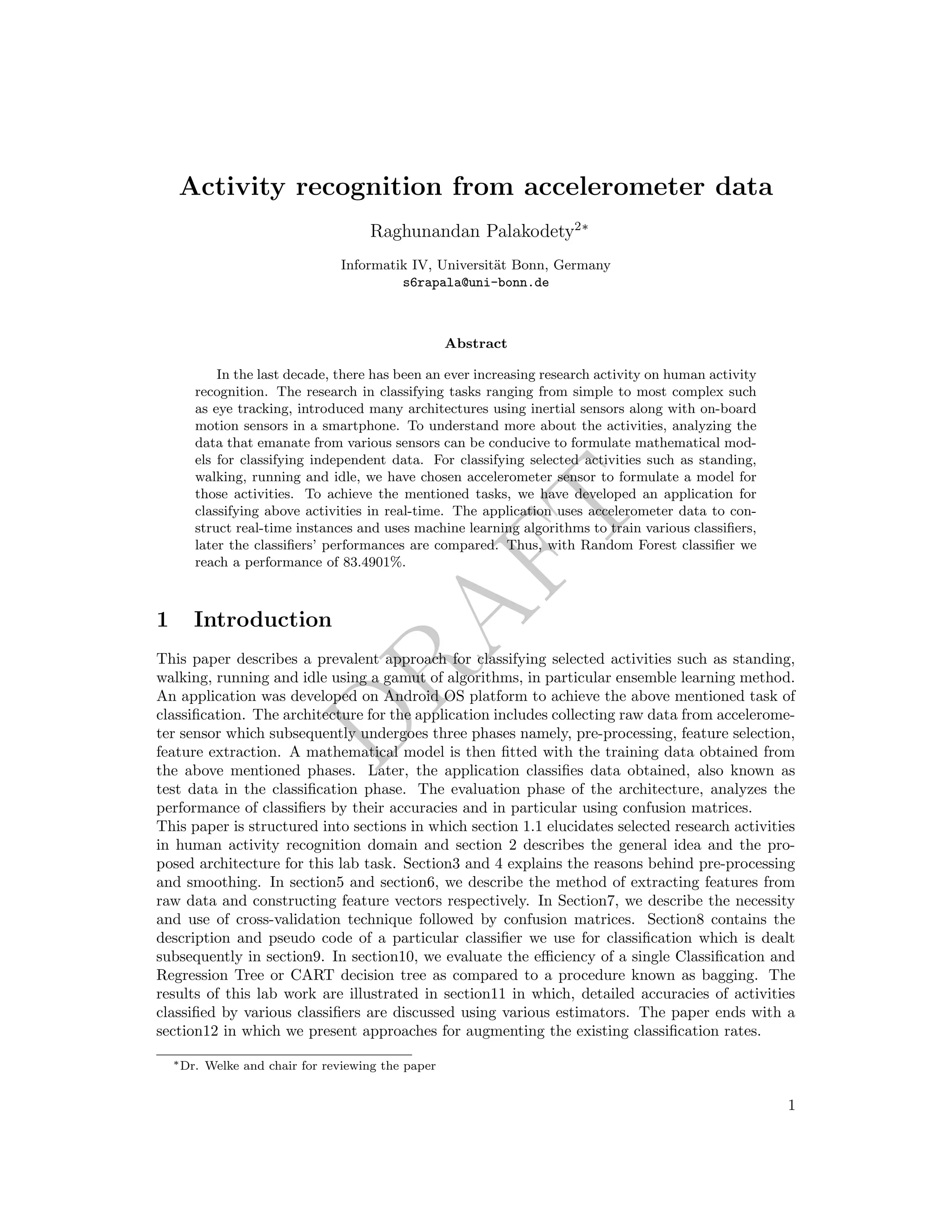
Standing Walking Running Others
703 1057 824 668
Table 1: Class distribution
a0 = 1−α
2 , a1 = 1
2 and a2 = α
2
and the equation,
w(n) = 0.42 − 0.5 cos((2πn)/(N − 1)) + 0.08 cos((4πn)/(N − 1))
5.2 Fourier Co-efficient representation in magnitude
It is important not to ignore the issue of time (phase) shifts when using Fourier analysis, since
the calculated Fourier co-efficients are very sensitive to time (phase) shifts. It is proven that
time (phase) shifting does not impact the Fourier series magnitude. Using this lemma, Fourier
co-efficients can be represented in terms of magnitude and phase as follows,
ˆXn = An + jBn and | ˆXn| = A2
n + B2
n
where ˆXn is the Fourier transform of a discrete signal and An and Bn are Fourier co-efficients.
6 Training data
The training data is constructed from the x, y, z sensor data readings as explained in section
5. After smoothing, the magnitude of these readings are collected in a blocked queue of size
2048. A background process is established by using AsyncTask (provided by the Android
framework), to use 64 buffered magnitude values before computing the Fast Fourier Transform
or FFT of these magnitude values.
The FFT using Blackman windowing function, computes the 64 FFT-coefficients. These coeffi-
cients along with maximum value of magnitude across all 64 individual magnitudes and label of
activity, serve as attributes or features for each feature vector or instance of the training data,
for that particular activity. The data is then saved as a file upon quitting the data acquisition
activity.
The file is of type Attribute-Relation File Format or arff. This file format is then analyzed by
Waikato Environment for Knowledge Analysis or WEKA, a knowledge analysis and machine
learning tool for further estimator values to peruse.
In the journal [18], evaluations were performed on datasets with both balanced and imbalanced
class distributions. It is observed in [18], where balanced class distribution data set of training
samples for each activity is collected, and this procedure was followed. Skewed set of samples
per activity were collected and subsequently analyzed in further stages of the pipeline. The
distribution of the training data is shown as bar plot in figure 8 and in table 1.
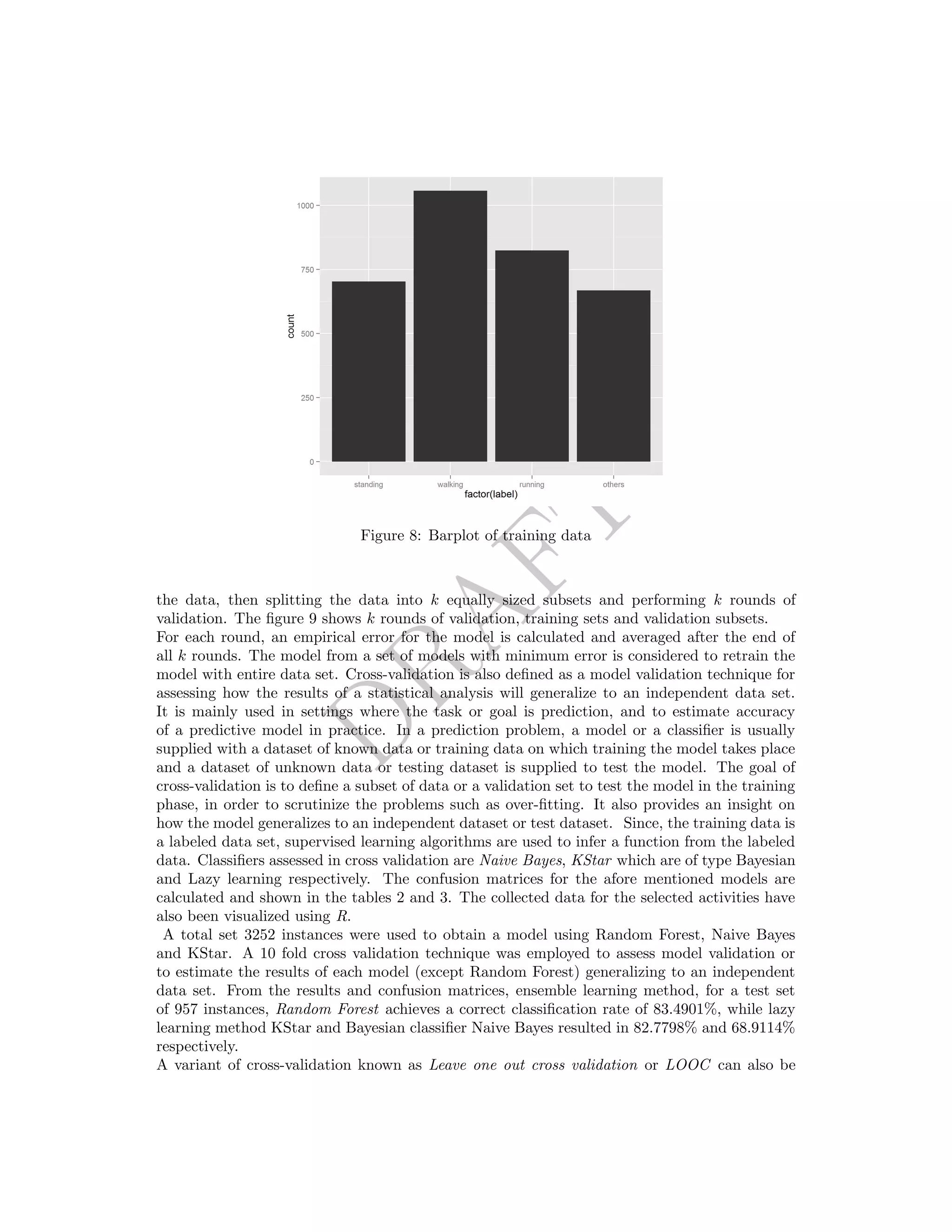
7 Cross-validation Results
Cross validation is a non-bayesian technique (for model selection) for choosing the model with
smallest empirical error on the validation set [12]. The technique involves randomly permuting

9. DRAFTFigure 8: Barplot of training data
the data, then splitting the data into k equally sized subsets and performing k rounds of
validation. The figure 9 shows k rounds of validation, training sets and validation subsets.
For each round, an empirical error for the model is calculated and averaged after the end of
all k rounds. The model from a set of models with minimum error is considered to retrain the
model with entire data set. Cross-validation is also defined as a model validation technique for
assessing how the results of a statistical analysis will generalize to an independent data set.
It is mainly used in settings where the task or goal is prediction, and to estimate accuracy
of a predictive model in practice. In a prediction problem, a model or a classifier is usually
supplied with a dataset of known data or training data on which training the model takes place
and a dataset of unknown data or testing dataset is supplied to test the model. The goal of
cross-validation is to define a subset of data or a validation set to test the model in the training
phase, in order to scrutinize the problems such as over-fitting. It also provides an insight on
how the model generalizes to an independent dataset or test dataset. Since, the training data is
a labeled data set, supervised learning algorithms are used to infer a function from the labeled
data. Classifiers assessed in cross validation are Naive Bayes, KStar which are of type Bayesian
and Lazy learning respectively. The confusion matrices for the afore mentioned models are
calculated and shown in the tables 2 and 3. The collected data for the selected activities have
also been visualized using R.
A total set 3252 instances were used to obtain a model using Random Forest, Naive Bayes
and KStar. A 10 fold cross validation technique was employed to assess model validation or
to estimate the results of each model (except Random Forest) generalizing to an independent
data set. From the results and confusion matrices, ensemble learning method, for a test set
of 957 instances, Random Forest achieves a correct classification rate of 83.4901%, while lazy
learning method KStar and Bayesian classifier Naive Bayes resulted in 82.7798% and 68.9114%
respectively.
A variant of cross-validation known as Leave one out cross validation or LOOC can also be

10. DRAFT
Figure 9: k-Fold Cross Validation
Confusion Matrix : Naive Bayes
Class
Label
Standing Walking Running Others
Standing 158 91 35 419
Walking 157 751 43 106
Running 1 151 671 1
Others 4 2 1 661
Table 2: Confusion Matrix for Naive Bayes
used to compute the mean squared error which is shown below as an equation. k-Fold cross-
validation procedure is LOOC when the parameter k is made equal to the number of instances
or data set. Under this setting, the bias becomes low, whereas the variance becomes high.
RMSE =
1
n
n
i=1
(yi − ˆyi)2,
where y is the observed value, ˆy is the predicted value and n is the number of folds. In case of
LOOC it is k = n.
7.1 Random Subspace
In the case of Random Forest of 10 trees, each constructed while considering 7 random
features gives an out of bag error estimate 0.1018. For 66 attribute feature vector, the number
of attributes considered for splitting at each node in a tree is calculated as follows,
K = ln(numberofattributes) + 1
From the above equation, the number of features or attributes is 7. This means, that the

11. DRAFT
Confusion Matrix : KStar
Class
Label
Standing Walking Running Others
Standing 544 67 5 87
Walking 212 832 4 9
Running 35 122 667 0
Others 16 2 1 649
Table 3: Confusion Matrix for KStar
random subset of 7 features define subspace of 65 dimensional space.
7.2 Out-of-bag Error Estimate in Random Forests
While using the random forests, cross validation technique to get an unbiased estimate error is
not required [4]. The error is calculated internally, as each tree is constructed using a different
bootstrap sample 8.1 from the original data. About one-third of the cases are left out of the
bootstrap sample and not used in the construction of kth
tree.
Out of 3252 size of bootstrap sample, 2068 unique statistical units are included in the bootstrap
sample and the rest (approximately 1/3rd
) serve as out of bag individuals. This can be visualized
using R’s association rules and frequent item set mining package, arules. The package provides a
generic function sample which produces sample (indices) of the specified size from the elements
provided using either with or without replacement.
The oob out-of-bag data is used to get a running unbiased estimate of the classification error
as trees are added to the forest. In this way, a test set classification is obtained for each case in
about one-third of the trees. At the end of the run, considering j to be the class that received
most of the votes every time case n was out-of-bag. The proportion of times that j is not equal
to the true class of n averaged over all the cases is the out-of-bag error estimate[4].
8 Training the Classifier
Random forests comprise CART like procedure and bootstrap aggregation or bagging along with
random subspaces method. In the supervised learning setting, B = 500 trees are constructed
or fitted, of which for each tree is grown on a bootstrap sample Di. Each sample generated
from the data set D (N points are sampled uniformly), with replacement from the set D is
termed as bagging. A tree Ti is grown using Di, such that at each node of the tree, a random
subset of features m or attributes is chosen and splitting is done only on those m features.
From section 5, each feature vector or instance constitutes 65 features, m 65. At the end
of constructing or growing B trees, given an unknown instance or a feature vector, a majority
vote is considered in case of classifying activity labels (not regression).
8.1 Bootstrap sampling
Bootstrap or re-sampling is a technique for improving the quality of estimators.
Bootstrap Algorithm

12. DRAFT
• Generate N bootstrap samples D1, D2, D3, .....,DN . Each bootstrap sample is obtained
by sampling n times with replacement from sample dataset. (Instances or data points
can appear multiple times in any Di).
• Evaluate the estimator on each bootstrap sample :
ˆSi = ˆS(Di)
that is estimate S pretending that Bi is the data.
• Compute the bootstrap estimate of S by averaging over all bootstrap samples.
ˆSBS = 1
|N|
N
i=1
ˆSi
• For each b = 1, 2, 3, ...., B , generate a bootstrap sample Bb. In detail: For i = 1, 2, 3, ..., n:
– Sample an index j ∈ {1,2,3, ....,n}
– Set ¯xb
i = ¯xj and add it to Bb
• For each b, compute mean and variance estimates:
ˆµb = 1
n
n
i=1 ¯xb
i and σ2
= 1
n
n
i=1(¯xb
i − ˆµb)2
• Compute the bootstrap estimate:
ˆσ2
BS = 1
B
B
b=1 ˆσ2
b
8.2 Bagging or Bootstrap Aggregation
Training phase
1. Initialize the parameters
• D = ∅, the ensemble.
• B, the number of classifiers to train.
2. For k = 1, ., ., ., ., B
• Take a bootstrap sample Bk from B.
• Build a classifier Dk using Bk as the training set.
• Add the classifier to the current ensemble, D = D ∪ Dk.
3. Return D.
Classification phase
4. Run D1, ., ., ., DB on the input x.
5. The class with maximum number of votes is chosen as the label for x.

13. DRAFT
9 Classification
The random forest classifier is trained on the data set and the test data is obtained from a
background service when the application starts and simultaneously applies the model to classify
the those data. Using Weka machine learning library and R data analysis library, estimators
were analyzed and plotted. The plot in the figure 10 shows error against number of trees
constructed for various activities. It can be observed as the number of trees are added to the
forest, the error decreases. Section 11 elucidates details on the results.
Figure 10: Overall error of the model
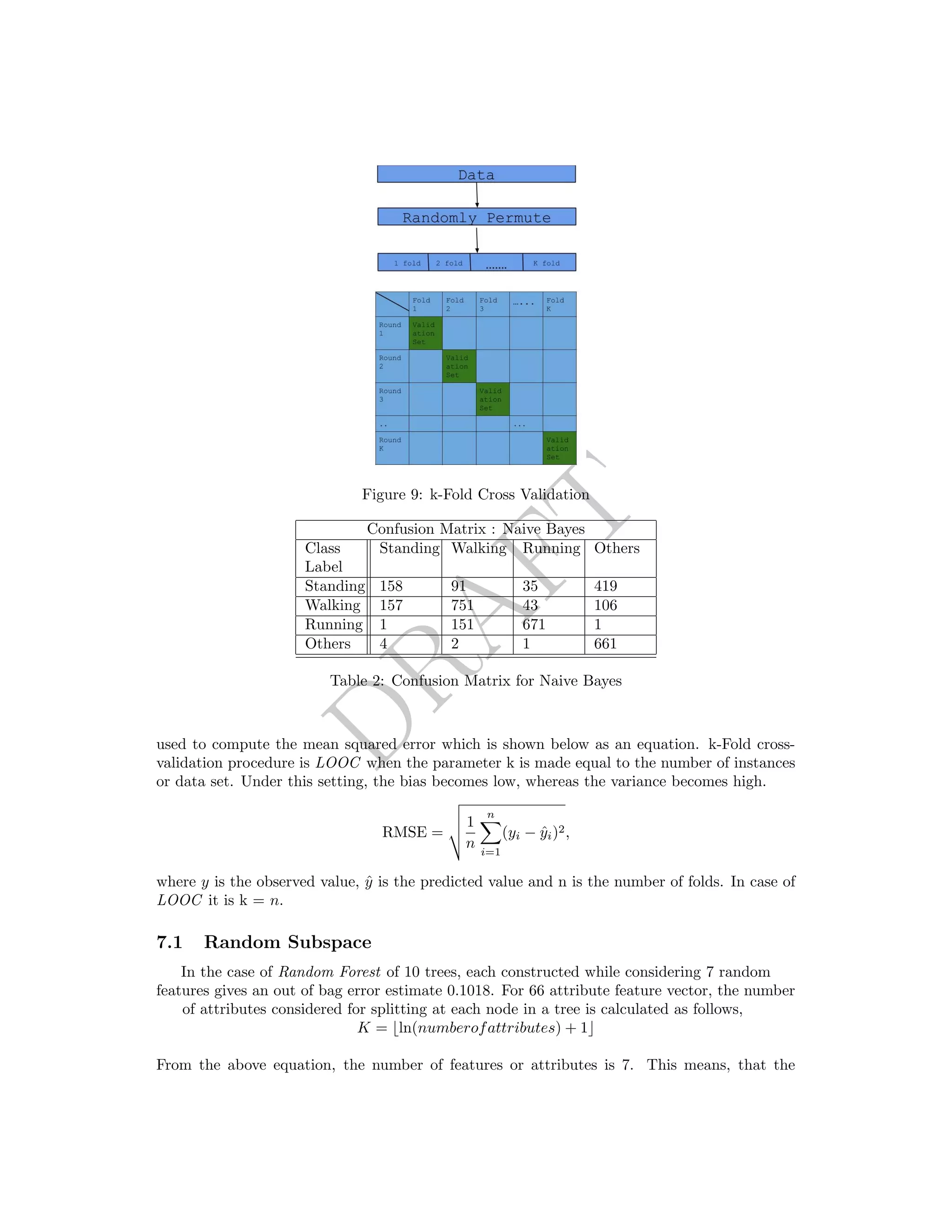
10 Comparison of non-linear predictive methods : Tree,
Bagging, Random Forest
Tree is a non linear method and is considered the basic building block for Bagging and Random
Forest
10.1 Tree
A single tree based prediction using CART as such, partitions the feature space into a set
of rectangles, on which predictions are assigned. Estimating VC dimension [3], multivariate
splitting criteria [10] and comparison of pruning methods [16] is beyond the scope of this paper.
R[22] offers a package rpart which essentially implements CART. The tree shown in figure 11
uses variable fft coef 0000 for construction of the tree with root node error 0.67497.

14. DRAFT
Figure 11: Tree : Variable used in tree construction fft coef 0000
Confusion Matrix : Random Forest
Class
Label
Standing Walking Running Others
Standing 126 3 4 3
Walking 90 380 6 0
Running 1 26 35 0
Others 24 1 0 258
Table 4: Confusion Matrix for Random Forest
10.2 Bagging
As mentioned in section 8.2 grows multiple trees, each grown on a different bootstrap sample
computed following the method in section 8.1. Since, the task is of type classification (certainly
not regression), a majority vote across all the trees is considered for prediction of the new
sample.
11 Results
For the random forest classifier, the confusion matrix 4 and the detailed accuracy including
Matthew’s correlation coefficient or MCC for all four activities computed are shown in the ta-
ble 5. Random forest of 10 trees, each constructed while considering 7 random features results
in out of bag error estimate 0.1018. Since, cross validation is ignored in the case of Random
forests, from the table 5, there still exists a possibility of over fitting on the training data.
From the results of various classifiers, random forest certainly outperformed in this task. Al-
though, the ’curse of dimensionality’ exists because 65 features for a feature vector, the results
prove to be satisfactory when compared to the rest of the classifiers. Out of 957 instances
supplied as test set, it is observed that 799 were correctly classified and rest 158 instances were
incorrectly classified. The lazy learning algorithm, KStar classified 653 instances correctly and
leaving 304 instances incorrectly classified while Naive Bayes has displayed a poor performance
of correctly classifying 564 instances and 393 instances incorrectly. One of the key statistic in

15. DRAFT
Detailed accuracy by class
Class
Label
TP
Rate
FP
Rate
Precision Recall F-
Measure
MCC
Standing 0.926 0.140 0.523 0.523 0.523 0.633
Walking 0.798 0.062 0.927 0.927 0.927 0.744
Running 0.565 0.011 0.778 0.778 0.778 0.643
Others 0.912 0.004 0.989 0.989 0.989 0.930
Weighted
Avg.
0.835 0.053 0.878 0.835 0.845 0.776
Table 5: Detailed accuracy by class
the results shown for random forest in table 5, is the MCC which serves as measure of quality
of binary classifications, where a perfect prediction value is +1 and -1 for total disagreement
between observed and predicted values.
To evaluate the performance of the classifiers Naive Bayes, KStar, and Random Forest for this
skewed dataset, it is necessary to peruse the cost sensitive analysis measure, ROC curve of the
mentioned classifiers. The area under the curve or AUC from the plots in figure 12, illustrates
the classification power of the classifier. It can be understood that more the area under the
curve, the better classification prowess the classifier possess. The point perfect classification
occurs at upper-left hand corner of the graph, at which True positive rate is 100% and false
positive rate is 0% which is impractical. From the plot in figure 12 it is conspicuous, for class
label standing, the roc space for Random Forest is greater than the rest of its counter parts and
appears fairly close to optimal.
Figure 12: Multiple ROC curves for class label ’Standing’

16. DRAFT
12 Conclusion
To achieve more effective classification values, Boosting can be used to improve the accuracy.
Much sophisticated techniques such as using temporal probabilistic models has been shown to
perform well in activity recognition and generally outperform non-temporal models [19]. Such
algorithms are used in advanced sensor fusion techniques where the tasks of classification are
more complex. The advent of incremental classifiers such as Hoeffding tree [15], an example of
Very Fast Decision Tree or VFDT, considerably learns better in case of massive data streams. In
the feature selection algorithm, there are various measures such as InfoGain and Ranker search
method to rank features of the vector, thus reducing the search space significantly. Allowing
various new measures and classification techniques can result in high classification rates and
hence the accuracy.
References
[1] Low pass filter smoothing sensor data with a low-pass filter. http://blog.thomnichols.org/
2011/08/smoothing-sensor-data-with-a-low-pass-filter.
[2] Motion Sensors api guides. http://developer.android.com/guide/topics/sensors/sensors_
motion.html.
[3] Ozlem Asian, Olcay Taner Yildiz, and Ethem Alpaydin. Calculating the vc-dimension of decision
trees. In Computer and Information Sciences, 2009. ISCIS 2009. 24th International Symposium
on, pages 193–198. IEEE, 2009.
[4] Leo Breiman. Random forests. Machine learning, 45(1):5–32, 2001.
[5] Andreas Bulling, Ulf Blanke, and Bernt Schiele. A tutorial on human activity recognition using
body-worn inertial sensors. ACM Computing Surveys, to appear 2014.
[6] Andrew T. Campbell. Smartphone Programming. http://www.cs.dartmouth.edu/~campbell/
cs65/myruns/myruns_manual.html#chap:labs:3, 2013. [Online; accessed 21-June-2014].
[7] Sauvik Das, LaToya Green, Beatrice Perez, Michael Murphy, and A Perring. Detecting user
activities using the accelerometer on android smartphones. The Team for Research in Ubiquitous
Secure Technology, TRUST-REU Carnefie Mellon University, 2010.
[8] Android Developer. Sensor Coordinate System. http://developer.android.com/guide/topics/
sensors/sensors_overview.html, 2014. [Online; accessed 10-June-2014].
[9] Irina Diaconita, Andreas Reinhardt, Frank Englert, Delphine Christin, and Ralf Steinmetz. Do
you hear what i hear? using acoustic probing to detect smartphone locations. In Proceedings of
the 1st Symposium on Activity and Context Modeling and Recognition (ACOMORE), pages 1–9,
Mar 2014.
[10] Richard O Duda, Peter E Hart, and David G Stork. Pattern classification. John Wiley & Sons,
2012.
[11] Manhyung Han, La The Vinh, Young-Koo Lee, and Sungyoung Lee. Comprehensive context
recognizer based on multimodal sensors in a smartphone. Sensors, 12(9):12588–12605, 2012.
[12] Trevor Hastie, Robert Tibshirani, and Jerome Friedman. The elements of statistical learning,
volume 2. Springer.
[13] Clemens Holzmann and Michael Haslgr¨ubler. A self-organizing approach to activity recognition
with wireless sensors. In Proceedings of the 4th International Workshop on Self-Organizing Systems
(IWSOS 2009), ETH Zurich, Switzerland, December 2009. Springer LNCS.
[14] Seyed Amir Hoseini-tabatabaei, Alexander Gluhak, and Rahim Tafazolli. A survey on smartphone-
based systems for opportunistic user context recognition. ACM Computing Surveys, 45(3), 2013.
[15] Geoff Hulten, Laurie Spencer, and Pedro Domingos. Mining time-changing data streams. In ACM
SIGKDD Intl. Conf. on Knowledge Discovery and Data Mining, pages 97–106. ACM Press, 2001.

17. DRAFT
[16] Oded Maimon and Lior Rokach. Data Mining and Knowledge Discovery Handbook. Springer-Verlag
New York, Inc., Secaucus, NJ, USA, 2005.
[17] B. P.; Teukolsky S. A.; Press, W. H.; Flannery and W. T Vetterling. Numerical recipes in fortran:
The art of scientific computing, 2nd ed. , cambridge univ. Press, Cambridge, pages 407–411, 1989.
[18] Muhammad Shoaib, Hans Scholten, and P.J.M. Havinga. Towards physical activity recognition
using smartphone sensors. In 10th IEEE International Conference on Ubiquitous Intelligence and
Computing, UIC 2013, pages 80–87, Los Alamitos, CA, USA, December 2013. IEEE Computer
Society.
[19] T.L.M. van Kasteren, G. Englebienne, and B.J.A. Krse. Human activity recognition from wireless
sensor network data: Benchmark and software. In Liming Chen, Chris D. Nugent, Jit Biswas,
and Jesse Hoey, editors, Activity Recognition in Pervasive Intelligent Environments, volume 4 of
Atlantis Ambient and Pervasive Intelligence, pages 165–186. Atlantis Press, 2011.
[20] Weka. Serialization. http://weka.wikispaces.com/Serialization, 2009. [Online; accessed 19-
July-2014].
[21] Xiaochao Yang, Chuang-Wen You, Hong Lu, Mu Lin, Nicholas D Lane, and Andrew T Camp-
bell. Visage: A face interpretation engine for smartphone applications. In Mobile Computing,
Applications, and Services, pages 149–168. Springer, 2013.
[22] Yanchang Zhao. Decision Trees. http://www.rdatamining.com/examples/decision-tree, 2014.
[Online; accessed 10-August-2014].