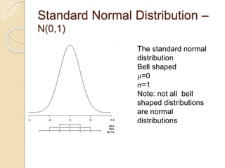
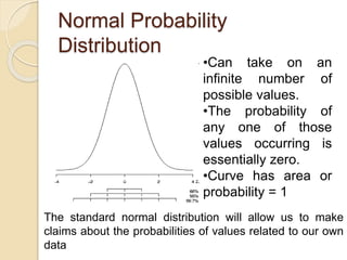
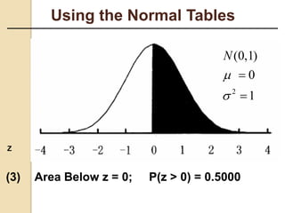
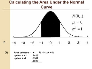
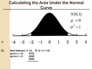
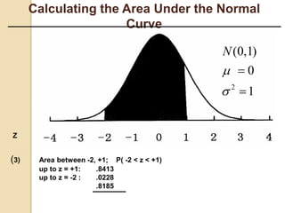
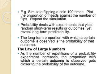
Chapter two of 'Econometrics for Development Professionals' covers essential statistical foundations including probability, random variables, and probability distributions. It discusses key concepts such as the law of large numbers, properties of normal distributions, and how probabilities relate to cumulative distribution functions. The chapter aims to equip professionals with the statistical tools necessary for development work, particularly in interpreting data and making informed decisions based on statistical inferences.

1. Econometrics for
Development Professionals
Chapter Two
Statistical Background
Zemen Ayalew (PhD)

2. Contents of this chapter
 Probability
 Random variables and Probability Distributions
 The Normal Probability Distributions and
Related Distributions
 Sampling Distributions for Samples from a
Normal Population
 Classical Statistical Inferences
 Properties of Estimators
 Testing of Hypotheses
 Relationship between Confidence Interval
Procedures and Tests of Hypotheses.

3. Probability
Probability is the study of random events.
The probability, or chance, that an event will happen can
be described by a number between 0 and 1:
•A probability of 0, or 0%, means the event has no
chance of happening.
•A probability of 1/2 , or 50%, means the event is just as
likely to happen as not to happen.
•A probability of 1, or 100%, means the event is certain
to happen.
Probability is a measure of the likelihood of a random
phenomenon or chance behavior. Probability describes
the long-term proportion with which a certain outcome
will occur in situations with short-term uncertainty.

4.  E.g. Simulate flipping a coin 100 times. Plot
the proportion of heads against the number of
flips. Repeat the simulation.
 Probability deals with experiments that yield
random short-term results or outcomes, yet
reveal long-term predictability.
 The long-term proportion with which a certain
outcome is observed is the probability of that
outcome.
The Law of Large Numbers
 As the number of repetitions of a probability
experiment increases, the proportion with
which a certain outcome is observed gets
closer to the probability of the outcome.

5.  In probability, an experiment is any process that
can be repeated in which the results are uncertain.
 A simple event is any single outcome from a
probability experiment. Each simple event is
denoted ei.
 The sample space, S, of a probability experiment is
the collection of all possible simple events. In other
words, the sample space is a list of all possible
outcomes of a probability experiment.
 An event is any collection of outcomes from a
probability experiment. An event may consist of one
or more simple events. Events are denoted using
capital letters such as E.
 The probability of an event, denoted P(E), is the
likelihood of that event occurring.

6. Properties of Probabilities
1. The probability of any event E, P(E), must be
between 0 and 1 inclusive. That is,
0 < P(E) < 1.
2. If an event is impossible, the probability of the
event is 0.
3. If an event is a certainty, the probability of the
event is 1.
4. If S = {e1, e2, …, en}, then
P(e1) + P(e2) + … + P(en) = 1.

7. Random Variables
 Random Variable (RV): A numeric
outcome that results from an experiment
Discrete random variables:
Finite discrete random variables were
ones in which the values were countable
whole numbered values. e.g.
◦ Number of sales
◦ Number of calls
◦ Shares of stock
◦ People in line
◦ Mistakes per page

8. Random Variables
 A continuous random variable is a
random variable that can assume any
value in some interval of numbers,
and are thus NOT countable.
◦ Examples:
 Continuous random variables
◦ Length
◦ Depth
◦ Volume
◦ Time
◦ Weight

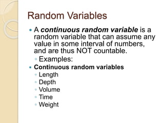
9. Continuous Random Variables
 A random variable is said to be continuous if there is a
function fX(x) with the following properties:
◦ Domain: all real numbers
◦ Range: fX(x)≥0
◦ The area under the entire curve is 1
 Such a function fX(x) is called the probability density
function (abbreviated p.d.f.)
 The fact that the total area under the curve fX(x) is 1 for all
X values of the random variable tells us that all
probabilities are expressed in terms of the area under the
curve of this function.
◦ Example: If X are values on the interval from [a,b], then
the P(a≤X≤b) = area under the graph of fX(x) over the
interval [a,b]
A
a b
fX

10. Probability Distributions
 Discrete Probability Distribution: Assigns
probabilities (masses) to the individual
outcomes
 Continuous Probability Distribution:
Assigns density at individual points,
probability of ranges can be obtained by
integrating density function
 Discrete Probabilities denoted by: p(y) =
P(Y=y)
 Continuous Densities denoted by: f(y)
 Cumulative Distribution Function: F(y) =
P(Y≤y)

11. Continuous Random
Variables
 Because all probabilities for a continuous
random variable are described in terms of
the area under the p.d.f. function, the
P(X=x) = 0.
◦ Why: the area of the p.d.f. for a single value is
zero because the width of the interval is zero!
◦ That is, for any continuous random variable,
X, P(X = a) = 0 for every number a. This DOES
NOT imply that X cannot take on the value a, it
simply means that the probability of that event is
0.

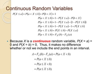
12. Continuous Random Variables
 Rather than considering the probability of X taking on a
given single value, we look for the probability that X
assumes a value in an interval.
 Suppose that a and b are real numbers with a < b.
Recall that X  a is the event that X assumes a value in
the interval(, a]. Likewise, a < X  b and b < X are the
events that X assumes values in (a, b] and (b, ),
respectively. These three events are mutually exclusive
and at least one of them must happen. Thus,
◦ P(X  a) + P(a < X  b) + P(b < X) = 1.
 Since we are interested in the probability that X takes a
value in an interval, we will solve for P(a < X  b).

13. Continuous Random Variables
 Because X is a continuous random variable, P(X = a) =
0 and P(X = b) = 0. Thus, it makes no difference
whether or not we include the end points in an interval.
     
     
     
 
     
     
  )
(
)
(
1
1
1
1
1
1
a
F
b
F
b
X
a
P
a
X
P
b
X
P
b
X
a
P
b
X
P
a
X
P
b
X
a
P
b
X
P
a
X
P
b
X
a
P
X
b
P
a
X
P
b
X
a
P
X
b
P
b
X
a
P
a
X
P
X
X 







































( ) ( ) ( )
( )
( )
( ).
X X
A F b F a P a X b
P a X b
P a X b
P a X b
    
  
  
  

14. The cumulative distribution function
 The same probability information is
often given in a different form, called
the cumulative distribution function,
(c.d.f), FX(x)
 FX(x)=P(Xx)
 0  FX(x) 1, for all x
 Domain is all real numbers

15. Normal Distribution
Why are normal distributions so
important?
 Many dependent variables are
commonly assumed to be normally
distributed in the population
 If a variable is approximately normally
distributed we can make inferences
about values of that variable
 Example: Sampling distribution of the
mean

16. Properties of normal distribution
 Symmetrical, bell-shaped curve
 Also known as Gaussian distribution
 Point of inflection = 1 standard
deviation from mean
 Mathematical formula
...
71828
.
2
e
and
...
14159
.
3
where
x
e
2
1
)
x
(
f
2
x
)
2
/
1
(






















17. Standard Normal Distribution –
N(0,1)
The standard normal
distribution
Bell shaped
=0
=1
Note: not all bell
shaped distributions
are normal
distributions

18. Normal Probability
Distribution
•Can take on an
infinite number of
possible values.
•The probability of
any one of those
values occurring is
essentially zero.
•Curve has area or
probability = 1
The standard normal distribution will allow us to make
claims about the probabilities of values related to our own
data

19. Z-score
If we know the population mean and
population standard deviation, for any
value of X we can compute a z-score
by subtracting the population mean
and dividing the result by the
population standard deviation
z 
X 


20. We can use the normal tables to obtain
probabilities for measurements for which this
frequency distribution is appropriate.
The table is a series of columns containing
numbers for z and for P(z). The z represents the
z-value for a normal distribution and P(z)
represents the area under the normal curve to
the left of that z-value for a normal distribution
with mean µ = 0 and standard deviation σ = 1.
Using the Normal Tables

21. Using the Normal Tables
Z
(1) Area Below z = -2; P(z < -2) = 0.0228
2
(0,1)
0
1
N





22. Using the Normal Tables
Z
2
(0,1)
0
1
N




(2) Area Below z = -1; P(z < -1) = 0.1587

23. Using the Normal Tables
Z
2
(0,1)
0
1
N




(1) Area Below z = +2; P(z > +2) = 0.0228

24. Using the Normal Tables
Z
2
(0,1)
0
1
N




(2) Area Below z = +1; P(z > +1) = 0.1587

25. Using the Normal Tables
2
(0,1)
0
1
N




(3) Area Below z = 0; P(z > 0) = 0.5000
Z

26. Calculating the Area Under the Normal
Curve
Z
2
(0,1)
0
1
N




(1) Area between -1, +1; P( -1 < z < +1)
up to z = +1: .8413
up to z = -1 : .1587
.6826

27. Calculating the Area Under the Normal
Curve
Z
2
(0,1)
0
1
N




(2) Area between -2, +2; P( -2 < z < +2)
up to z = +2: .9772
up to z = -2 : .0228
.9544

28. Calculating the Area Under the Normal
Curve
2
(0,1)
0
1
N




(3) Area between -2, +1; P( -2 < z < +1)
up to z = +1: .8413
up to z = -2 : .0228
.8185
Z

29. Standard Normal Distribution
2
(0,1)
0
1
N




(1) Values of z that bracket middle 95%
-1.96 to +1.96
Z

30. Standard Normal Distribution
2
(0,1)
0
1
N




(1) Values of z that bracket middle 99%
-2.576 to +2.576
Z

31. Calculating z-values
and ~ (0,1)
Z N
If ~ ( , )
x x
X N  
then the corresponding z value for x is given as
x
x
x
z




i.e. µz = 0 and z
2 = 1

32. ; if ~N( 150,10) . . 150, 10
150 150
when = 150; 0
10
170 150 20
when = 170; 2
10 10
x
x x
x
x
z X i e
x z
x z

 


  

 

  
Calculating z-values
2
~ (0,1)
0
1
z
z
Z N




Z
~ ( , )
150
10
x x
x
x
X N  




110 120 130 140 150 160 170 180
190 2
x x
 
 2
x x
 

1
x x
 

3
x x
 
 1
x x
 

x
 3
x x
 


33. The following questions reference a normal
distribution with a mean  = 150 lbs, a variance 2 =
100 lbs2, and a standard deviation  = 10 lbs. Such a
distribution is often indicated by the symbols N(,) =
N(150, 10).
1. What is the likelihood that a randomly selected
individual observation is within 5 lbs of the population
mean  = 150lbs?
2. What is the likelihood that a mean from a random
sample of size n = 5 is within 5 lbs of  = 150 lbs?
3. What is the likelihood that a mean from a random
sample of size n = 20 is within 5 lbs of  = 150 lbs?
Some Questions

34. Solution to Question 1
0.38292
X
155 150
0.5
10
Upper x
Upper
x
x
z


 
  
Area between z upper and z lower = 0.38292
145 150
0.5
10
Lower x
Lower
x
x
z


 
   
, Area up to z upper = 0.69146
, Area up to z lower = 0.30854
~ (150,10)
1
150
10
x
x
X N
n
lbs
lbs






35. Solution to Question 2
Area between z upper and z lower = 0.73728
0.7372
8
155 150
1.12
4.47
Upper x
Upper
x
x
z


 
  
145 150
1.12
4.47
Lower x
Lower
x
x
z


 
   
, Area up to z upper =
0.86864
, Area up to z lower =
0.13136
~ ( , )
5
150
10
4.47
5
x x
x
x
X N
n
n
 





  
X

36. Solution to Question 3
0.97490
155 150
2.24
2.23
Upper x
Upper
x
x
z


 
  
145 150
2.24
2.23
Lower x
Lower
x
x
z


 
   
, Area up to z upper =
0.98745
, Area up to z lower =
0.01255
Area between z upper and z lower = 0.97490
~ ( , )
20
150
2.23
x x
x
x
X N
n
lbs
lbs
n
 





 
X

37. 13 - 37
1
150
10
n
lbs
lbs





0.38292
5
150
= 4.47
x
n
lbs
lbs
n






20
150
= 2.23
x
n
lbs
lbs
n






0.7372
8
0.97490

38. •When centered about  = 150 lbs, what
proportion of the total distribution does an
interval of length 10 lbs cover?
• How many standard deviations long
must an interval be to cover the middle
95% of the distribution?
• From  - (??) standard deviations to  +
(??) standard deviations covers (??) % of
the distribution?
All these questions require that the value
for  be known and that it be placed in the
center of these “intervals”.
Some More Questions

39. A Sampling Distribution
The way our means would be distributed if we
collected a sample, recorded the mean and threw it
back, and collected another, recorded the mean and
threw it back, and did this again and again
A theoretical frequency distribution of the scores for or
values of a statistic, such as a mean. Any statistic that
can be computed for a sample has a sampling
distribution.
A sampling distribution is the distribution of statistics
that would be produced in repeated random sampling
(with replacement) from the same population.
It is all possible values of a statistic and their
probabilities of occurring for a sample of a particular
size.
Sampling distributions are used to calculate the
probability that sample statistics could have occurred
by chance and thus to decide whether something that is
true of a sample statistic is also likely to be true of a
population parameter.

40. Sampling Distribution
We are moving from descriptive statistics to
inferential statistics.
Inferential statistics allow the researcher to come to
conclusions about a population on the basis of
descriptive statistics about a sample.
For example:
Your sample says that a candidate gets support
from 47%.
Inferential statistics allow you to say that the
candidate gets support from 47% of the population
with a margin of error of +/- 4%.
This means that the support in the population is
likely somewhere between 43% and 51%.

41. A Sampling Distribution
Some rules about the sampling
distribution of the mean…
1. For a random sample of size n from a population having mean
 and standard deviation , the sampling distribution of Y-bar
(glitter-bar?) has mean  and standard error Y-bar = /n
2. The Central Limit Theorem says that for random sampling, as
the sample size n grows, the sampling distribution of Y-bar
approaches a normal distribution.
3. The sampling distribution will be normal no matter what the
population distribution’s shape as long as n > 30.
4. If n < 30, the sampling distribution is likely normal only if the
underlying population’s distribution is normal.
5. As n increases, the standard error (remember that this word
means standard deviation of the sampling distribution) gets
smaller.
6. Precision provided by any given sample increases as sample
size n increases.

42. The Binomial Distribution
 A Binomial Random Variable
◦ n identical trials
◦ Two outcomes: Success or Failure
◦ P(S) = p; P(F) = q = 1 – p
◦ Trials are independent
◦ x is the number of Successes in n trials
42

43. The Binomial Distribution
 A Binomial Random
Variable
◦ n identical trials
◦ Two outcomes: Success or
Failure
◦ P(S) = p; P(F) = q = 1 – p
◦ Trials are independent
◦ x is the number of S’s in n
trials
Flip a coin 3 times
Outcomes are Heads or
Tails
P(H) = .5; P(F) = 1-.5 =
.5
A head on flip i doesn’t
change P(H) of flip i +
1
43

44. The Binomial Distribution
Results of 3 flips Probability Combined Summary
HHH (p)(p)(p) p3 (1)p3q0
HHT (p)(p)(q) p2q
HTH (p)(q)(p) p2q (3)p2q1
THH (q)(p)(p) p2q
HTT (p)(q)(q) pq2
THT (q)(p)(q) pq2 (3)p1q2
TTH (q)(q)(p) pq2
TTT (q)(q)(q) q3 (1)p0q3
44

45. The Binomial Distribution
 The Binomial Probability Distribution
◦ p = P(S) on a single trial
◦ q = 1 – p
◦ n = number of trials
◦ x = number of successes
x
n
x
q
p
x
n
x
P 









)
(
45

46. The Binomial Distribution
 The Binomial Probability Distribution
x
n
x
q
p
x
n
x
P 









)
(
46

47.  Say 40% of the
class is female.
 What is the
probability that 6
of the first 10
students walking
in will be female?
The Binomial Distribution
1115
.
)
1296
)(.
004096
(.
210
)
6
)(.
4
(.
6
10
)
(
6
10
6





















x
n
x
q
p
x
n
x
P
47

48. The Binomial Distribution
Mean
Variance
Standard Deviation
 A Binomial Random Variable has
48
2
np
npq
npq







49. The Binomial Distribution
16
250
250
5
.
5
.
1000
500
5
.
1000
2












npq
npq
np



 For 1,000 coin flips,
The actual probability of getting exactly 500 heads out of 1000 flips is
just over 2.5%, but the probability of getting between 484 and 516 heads
(that is, within one standard deviation of the mean) is about 68%.
49