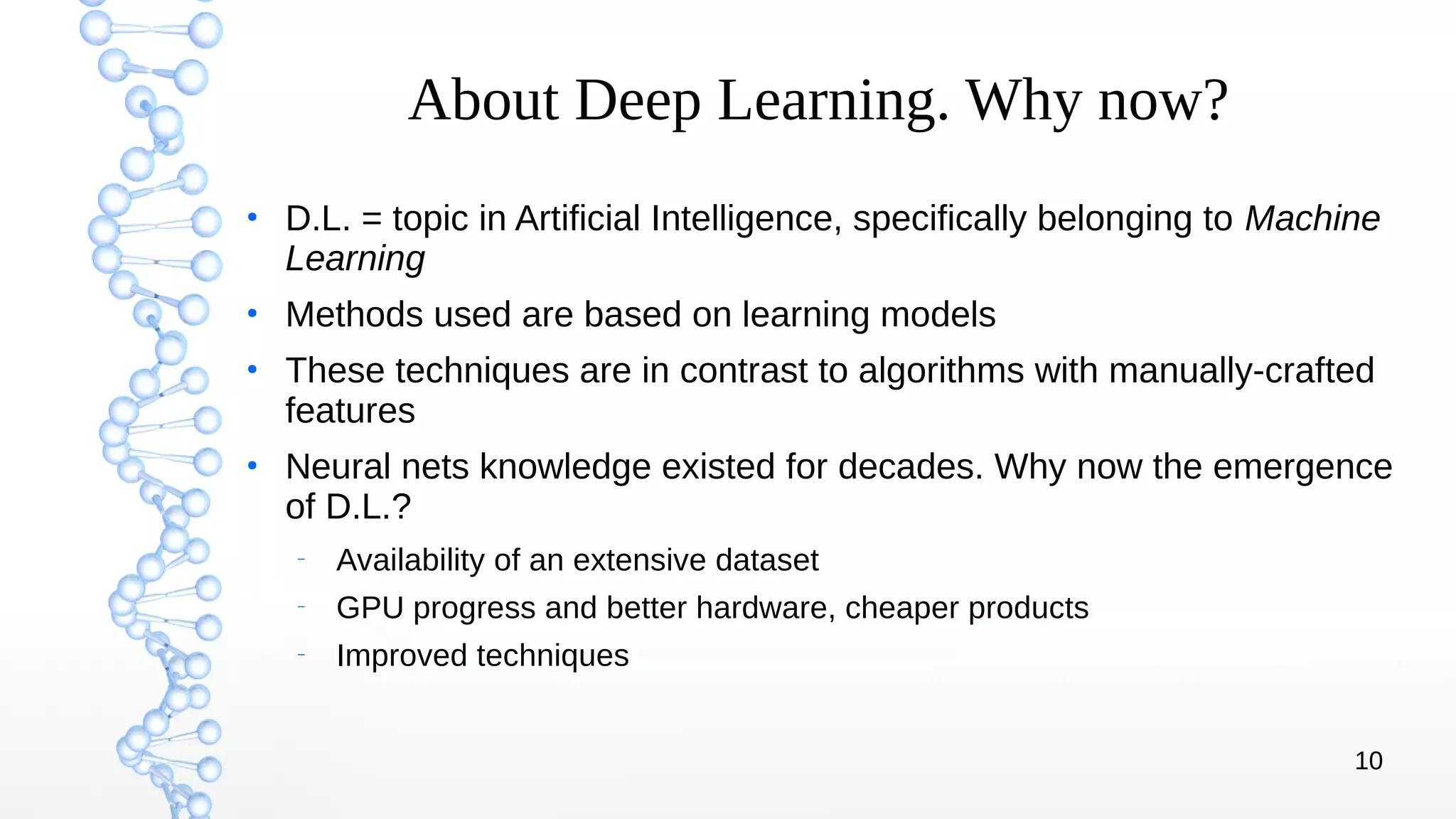
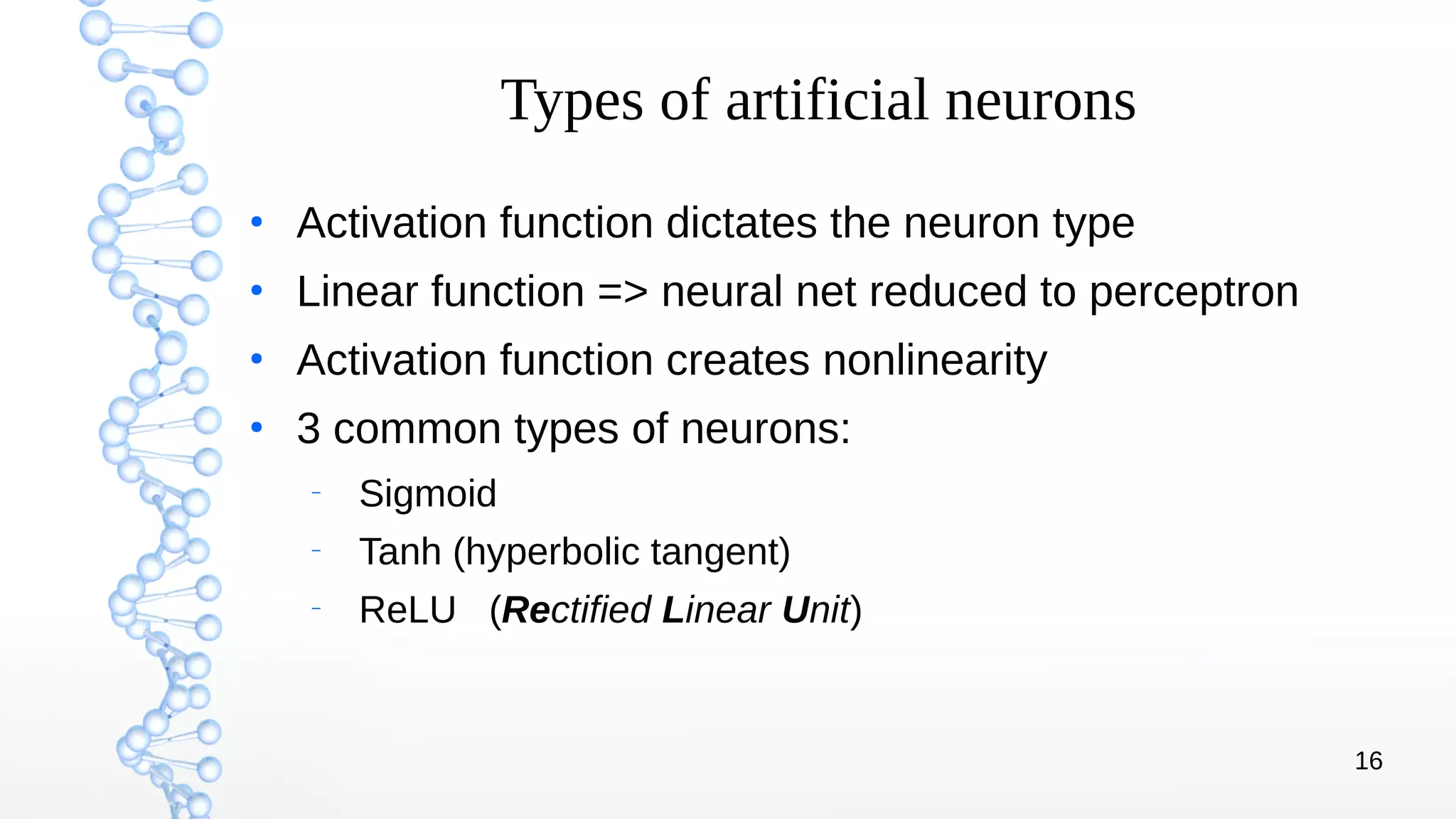
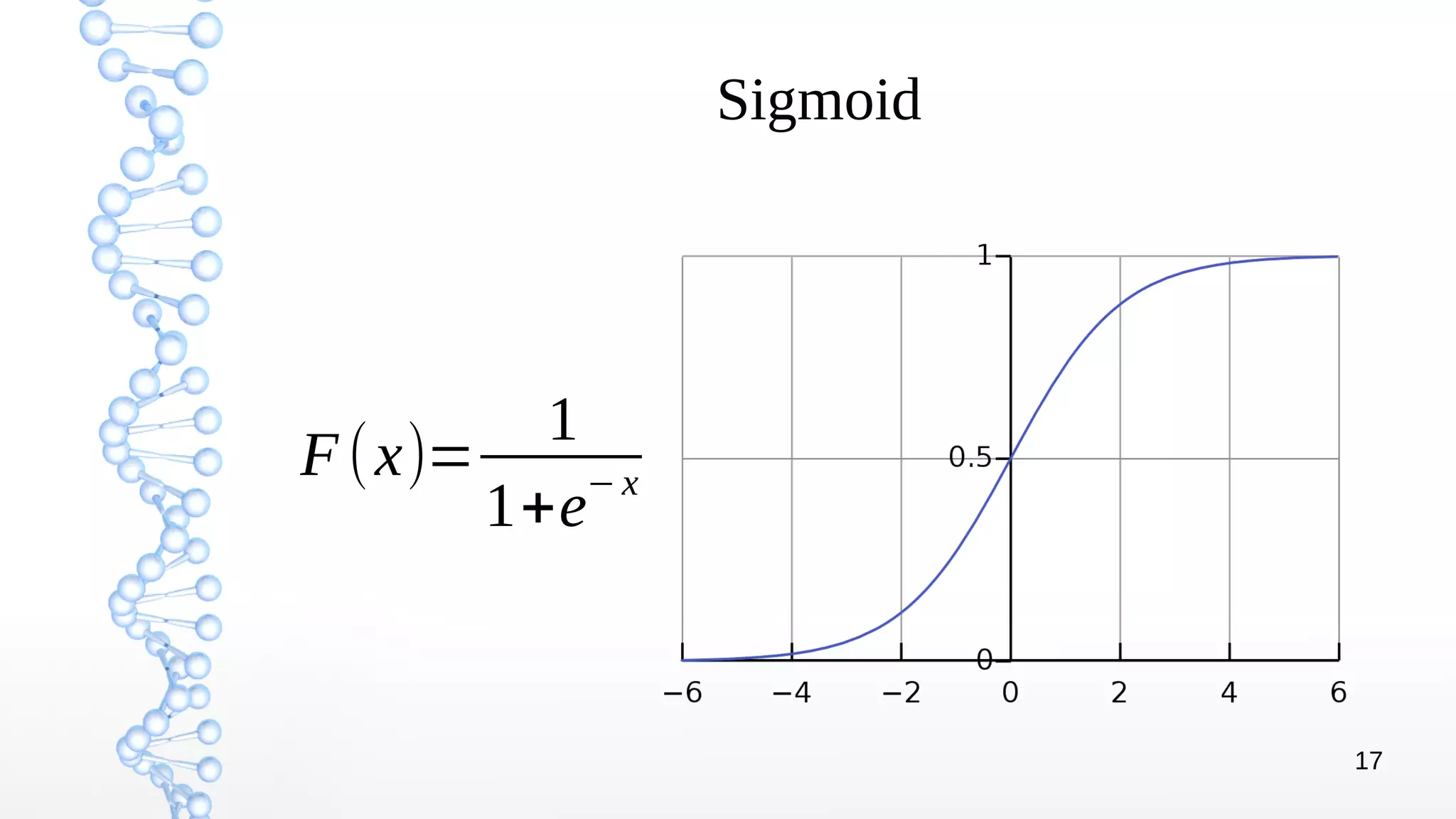
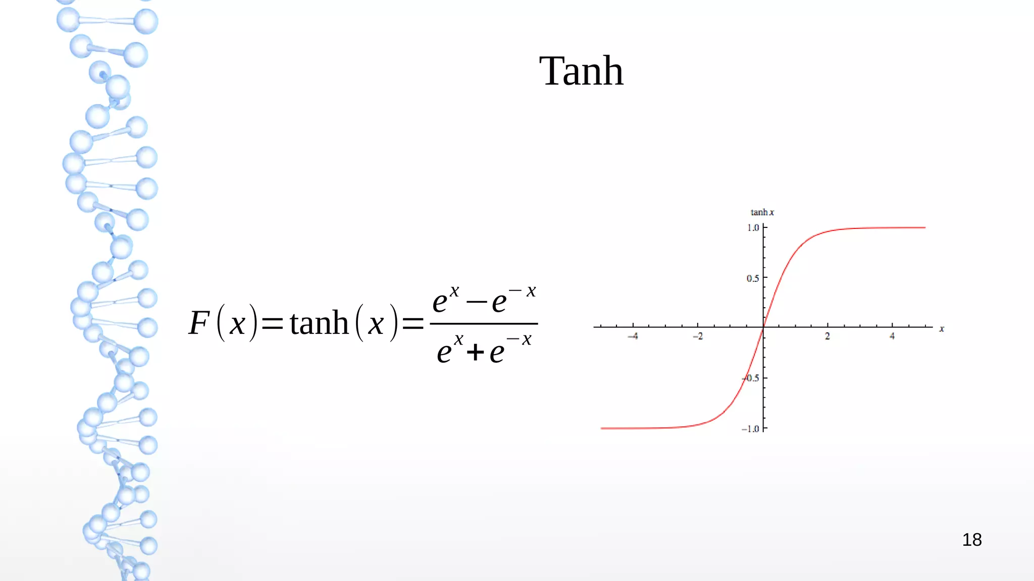
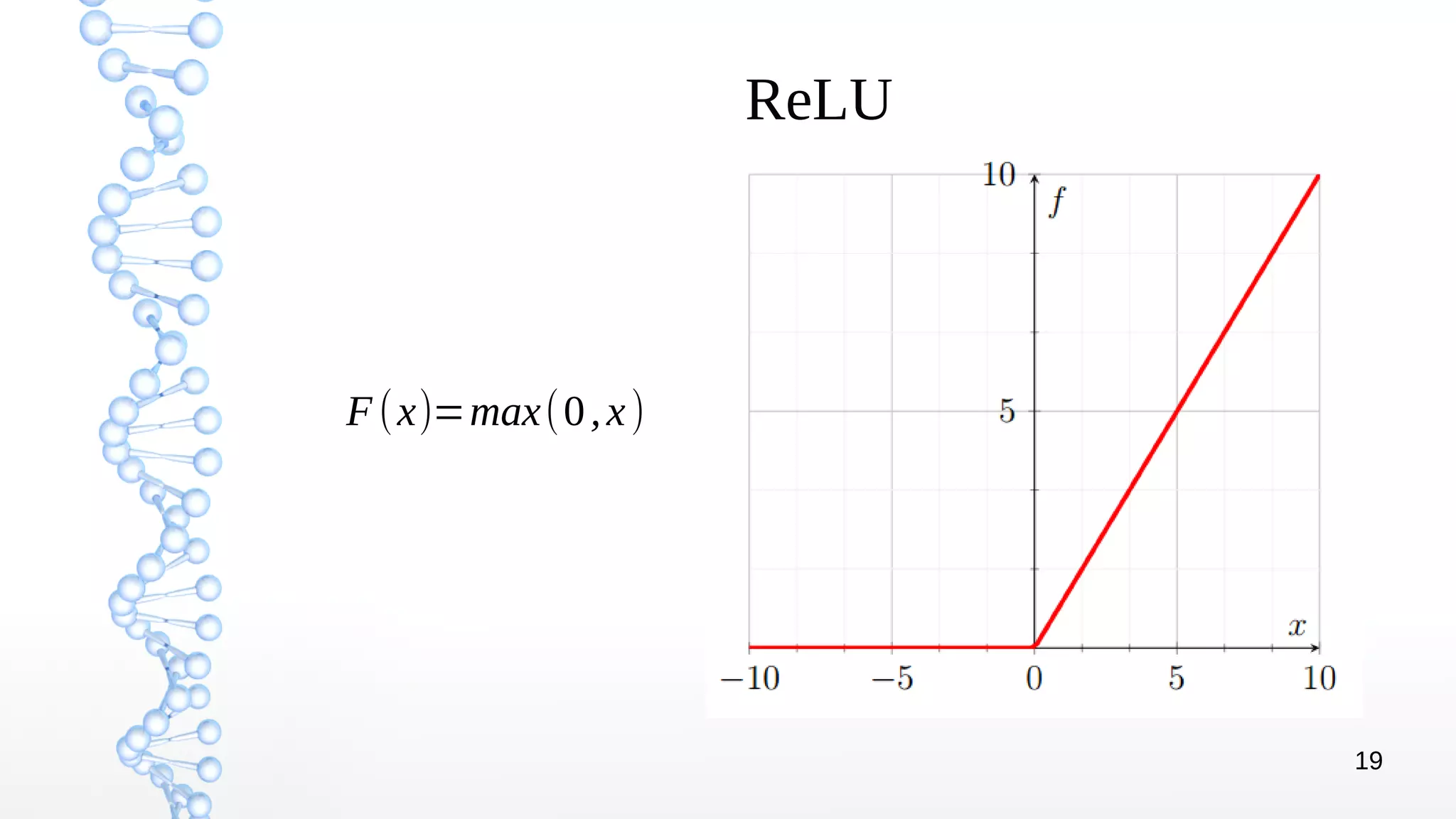
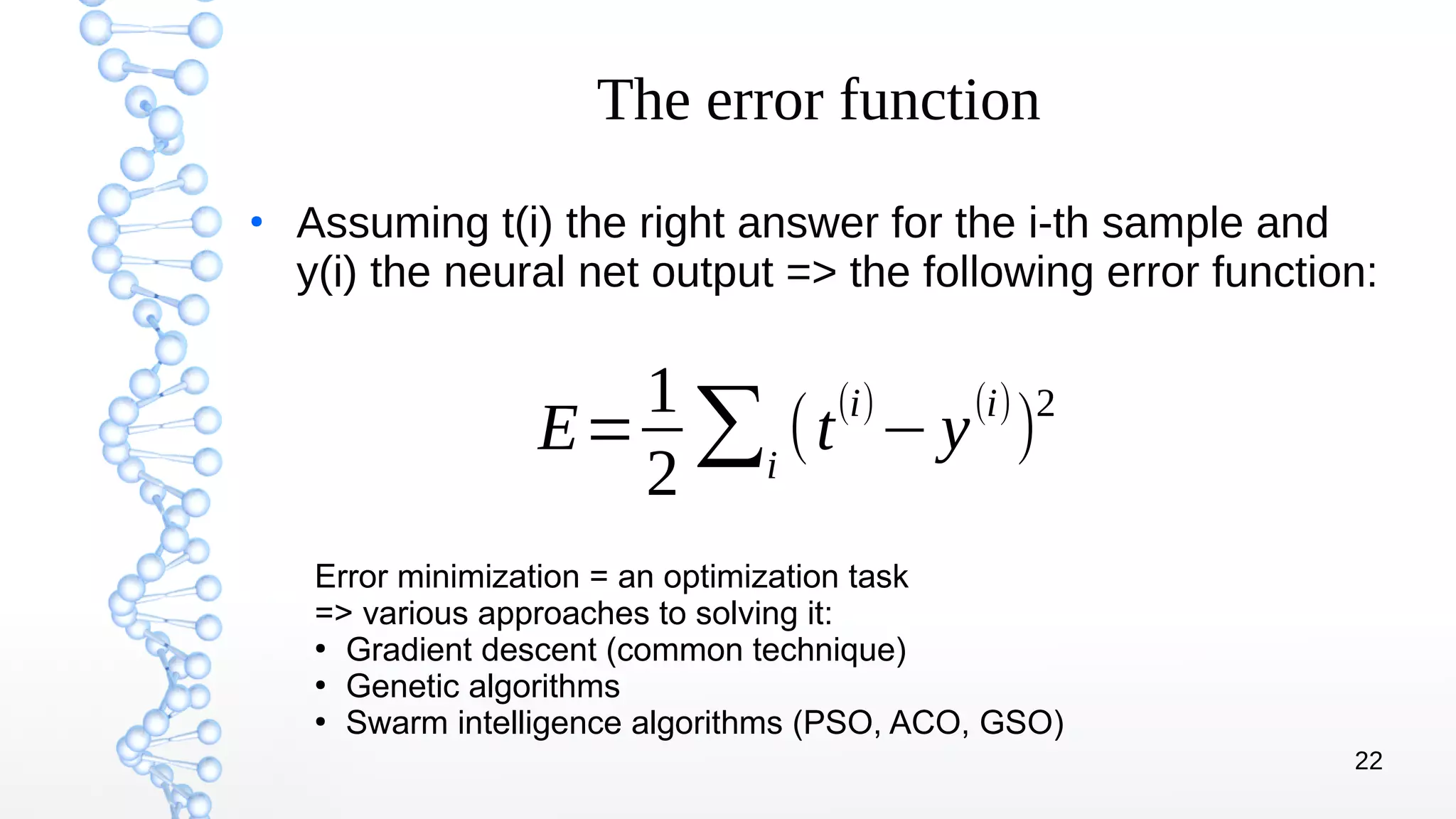
The document presents an introduction to deep learning, covering its theoretical concepts, frameworks, and applications in various fields such as robotics and computer vision. It details the evolution of deep learning techniques, the structure of artificial neural networks, and essential processes like backpropagation and gradient descent. The document also addresses artificial neuron types, learning processes, and the significance of convolutional neural networks for image processing.

1. 1
Deep Learning
Vlad Ovidiu Mihalca
PhD student – AI & Vision
Mechatronics @ University of Oradea
16th of January, 2018

2. 2
Series of talks
●
Part I: theoretical base concepts
●
Part II: frameworks and DL industry use
●
Part III: usage in robotics and Computer Vision, state of
the art in research

3. 3
2016 = Year of Deep Learning (1 / 7)

4. 4
2016 = Year of Deep Learning (2 / 7)

5. 5
2016 = Year of Deep Learning (3 / 7)

6. 6
2016 = Year of Deep Learning (4 / 7)

7. 7
2016 = Year of Deep Learning (5 / 7)

8. 8
2016 = Year of Deep Learning (6 / 7)

9. 9
2016 = Year of Deep Learning (7 / 7)

10. 10
About Deep Learning. Why now?
●
D.L. = topic in Artificial Intelligence, specifically belonging to Machine
Learning
●
Methods used are based on learning models
●
These techniques are in contrast to algorithms with manually-crafted
features
●
Neural nets knowledge existed for decades. Why now the emergence
of D.L.?
–
Availability of an extensive dataset
–
GPU progress and better hardware, cheaper products
–
Improved techniques

11. 11
Inspiration for D.L. models
●
The human brain
–
Comes with an initial model => approximates reality
–
While growing up => receives sensory inputs => approximates
the experience
●
External factors (= our parents)
–
Confirm or correct our approximations => the model is
reinforced / is adjusted
●
Similar ideas to the above inspired Machine Learning =>
self-adjusting models that learn from example

12. 12
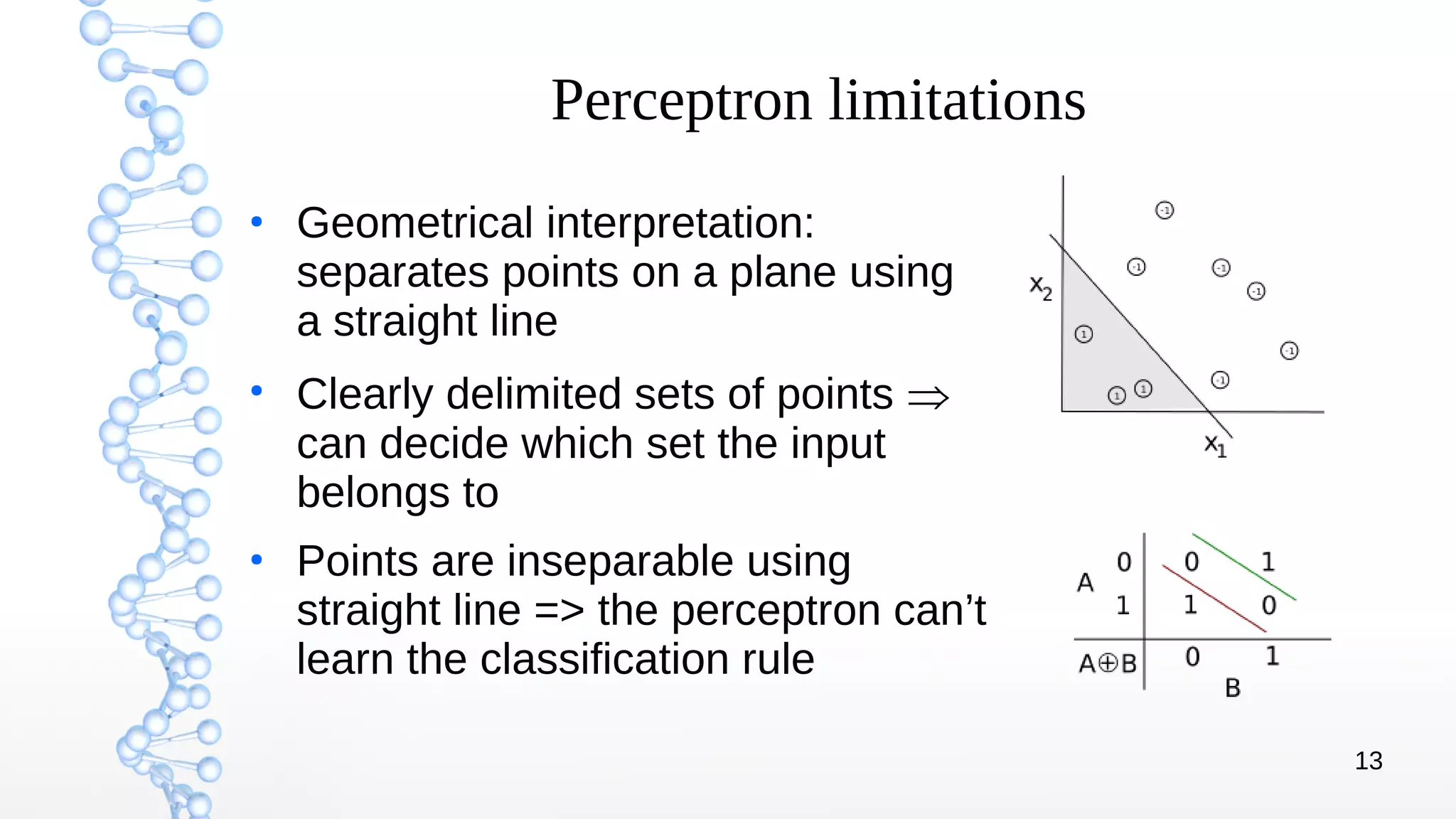
The linear perceptron
●
A simple learning model:
–
A mathematical function h(x, θ)
–
x = model input vector
–
θ = internal parameters vector
●
Example: an exam result guess model => above/below
average exam result – based on sleep hours and study
hours
h(x ,θ)=
{
−1,x
T
⋅
[θ 1
θ 2]+θ 0<0
1,xT
⋅
[θ 1
θ 2
]+θ 0≥0
x=[x1, x2]T
θ=[θ 1,θ 2,θ 0]T
x1
– sleep hours
x2
– study hours

13. 13
Perceptron limitations
●
Geometrical interpretation:
separates points on a plane using
a straight line
●
Clearly delimited sets of points 
can decide which set the input
belongs to
●
Points are inseparable using
straight line => the perceptron can’t
learn the classification rule

14. 14
Artificial neural nets
●
Biologically inspired structure, similar to the brain =>
connected artificial neurons
●
Connection = intensity & information flow direction
●
Neuron outputs = inputs for neurons in the following
layers

15. 15
Artificial neuron
●
Model that contains:
–
Weighted inputs
–
An output
–
Activation function
S=∑
i=1
n
xi wi
o=F(S)

16. 16
Types of artificial neurons
●
Activation function dictates the neuron type
●
Linear function => neural net reduced to perceptron
●
Activation function creates nonlinearity
●
3 common types of neurons:
–
Sigmoid
–
Tanh (hyperbolic tangent)
–
ReLU (Rectified Linear Unit)

17. 17
Sigmoid
F(x)=
1
1+e
− x

18. 18
Tanh
F(x)=tanh(x)=
ex
−e− x
e
x
+e
−x

19. 19
ReLU
F(x)=max(0,x)

20. 20
The learning process
●
Adjusting edge weights in an iterative way, to output
desired answers
●
Several techniques and algorithms
●
The backpropagation algorithm: ripple the difference
between result and objective backwards on previous
layers

21. 21
Backpropagation - outline
1) Use a vector as input => get result as output
2) Compare output with desired vector
3) The difference is propagated backwards in the net
4) Adjust weights according to an error-minimizing
algorithm

22. 22
The error function
●
Assuming t(i) the right answer for the i-th sample and
y(i) the neural net output => the following error function:
Error minimization = an optimization task
=> various approaches to solving it:
●
Gradient descent (common technique)
●
Genetic algorithms
●
Swarm intelligence algorithms (PSO, ACO, GSO)
E=
1
2
∑i
(t
(i)
−y
(i)
)
2

23. 23
Gradient descent
●
Assume 2 weights: w1 and w2 => XY plane made of
[w1, w2] pairs
●
Z axis: error value at [w1, w2] coordinates =>
somewhere on the graph surface
●
Need to descend on the slope towards a minimum point
●
Steepest curve = perpendicular line to level ellipse =>
descend on the gradient of the error function
Δ wk=−ϵ
∂ E
∂wk
=...=∑
i
ϵ xk
(i)
(t
(i)
− y
(i)
)
ϵ = learning rate xk(i) = k-th input of i-th sample
i = i-th sample t(i),y(i) = desired outcome / actual output

24. 24
Backpropagation & gradient descent
●
Weight adjustment în hidden layers:
–
Calculate error change depending on hidden outputs
–
Calculate error change depending on individual weights
●
For this we can use a dynamic programming approach
–
Store previously calculated values in a table and reuse them
as necessary

25. 25
Convolutional neural nets
●
Classical neural net density gets very large for images
●
Simplify graph by calculating a subgraph
●
Multiple filters are repeatedly applied to parts of the image
=> smaller array
●
The operation is known as convolution
●
It is a linear operation => nonlinearity is later added through
ReLU or sigmoids
●
The neural net trains on these feature maps
●
More details about these in a future session...

26. 26
Thank you for attending!

27. 27
Bibliography
●
MIT 6.S191 course: Intro to Deep Learning
●
Nikhil Buduma – Fundamentals of Deep Learning
●
Ecaterina Vladu – Inteligenţa artificială
●
Wikipedia. Deep learning