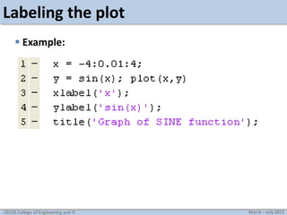
Download as PDF, PPTX
![Discrete signals
Plot the discrete signal x = [1 2 3 4] in MATLAB
4
3
2
1
-1
0
1
2
using stem(x) plots the signal starting from index number 1
CECOS College of Engineering and IT
March – July 2012](https://image.slidesharecdn.com/labno-140228005629-phpapp01/85/matab-no4-2-320.jpg)
![Practice
Plot the following discrete time sequences
x[n]=[1 1 1 1 2 1 1 1 1]
x[n]=[5 4 3 2 1 0 1 2 3 4 5]
CECOS College of Engineering and IT
March – July 2012](https://image.slidesharecdn.com/labno-140228005629-phpapp01/85/matab-no4-3-320.jpg)

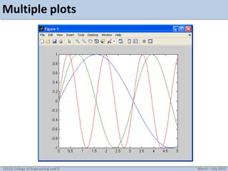
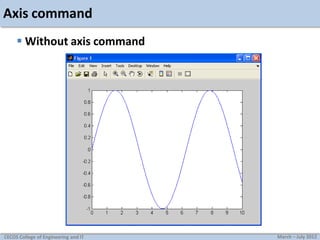
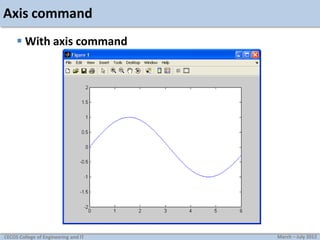
![Axis command
Used to manually zoom axis
axis([xmin xmax ymin ymax])
Example:
CECOS College of Engineering and IT
March – July 2012](https://image.slidesharecdn.com/labno-140228005629-phpapp01/85/matab-no4-14-320.jpg)
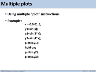
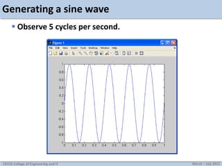
![Generating a sine wave
Example: creating a 5Hz sine wave, sampled at 8000Hz.
f=5;
fs=8000;
t=[0:1/fs:1];
y=sin(2*pi*f*t);
plot(t,y);
CECOS College of Engineering and IT
March – July 2012](https://image.slidesharecdn.com/labno-140228005629-phpapp01/85/matab-no4-19-320.jpg)
![Generating a sine wave
Example: Creating a 1000Hz sine wave, sampled at
8000Hz, and routing it to computer’s soundcard.
f=1000;
fs=8000;
t=[0:1/fs:3];
y=sin(2*pi*f*t);
sound(y,fs);
The sound will be heard for 3 seconds, as dictated by the code
CECOS College of Engineering and IT
March – July 2012](https://image.slidesharecdn.com/labno-140228005629-phpapp01/85/matab-no4-21-320.jpg)
![Task
1. Plot the two curves y1 = x2 and y2 = 2x on the same graph using
different plot styles. Label the plot properly
2. Write a MATLAB program that adds the following two signals,
Plot the original signals as well as their sum.
x1[n] = [2 2 2 2 2]
x2[n] = [2 2 2 2 0 0]
3. Scale the amplitude of the following signal by a factor of 2 and
½ and show the scaled signals along with the original.
x(t) = sin(t) + 1/3sin(3t)
CECOS College of Engineering and IT
,
t=0:0.01:10
March – July 2012](https://image.slidesharecdn.com/labno-140228005629-phpapp01/85/matab-no4-22-320.jpg)

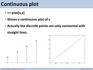
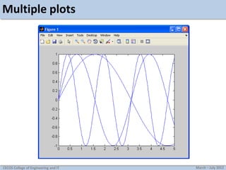
This document discusses MATLAB graphics and plotting discrete and continuous signals. It provides examples of plotting single and multiple signals, changing plot settings, using subplots, generating sine waves, and tasks for practicing MATLAB plotting. Key topics covered include using stem, plot, and hold on to display signals; setting line types and styles; manually zooming axes; creating subplots; and generating and playing sine waves with MATLAB.