Statistics Branches

1. DESCRIPTIVE &
INFERENTIAL STATISTICS
Dr. Ratnaprabha Jadhav (Prof & Head)
Department of Geography, PGSR,
SNDT Women’s University, Pune Campus

2. Precision, Accuracy, Validity, Reliability

4. RESEARCH DATA
RESEARCH DATA

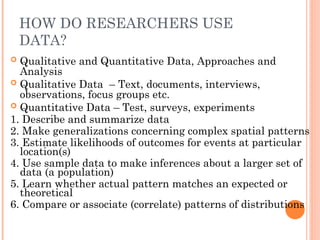
5. HOW DO RESEARCHERS USE
DATA?
 Qualitative and Quantitative Data, Approaches and
Analysis
 Qualitative Data – Text, documents, interviews,
observations, focus groups etc.
 Quantitative Data – Test, surveys, experiments
1. Describe and summarize data
2. Make generalizations concerning complex spatial patterns
3. Estimate likelihoods of outcomes for events at particular
location(s)
4. Use sample data to make inferences about a larger set of
data (a population)
5. Learn whether actual pattern matches an expected or
theoretical
6. Compare or associate (correlate) patterns of distributions

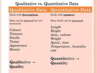
6. Qualitative vs. Quantitative Data
Qualitative vs. Quantitative Data
Qualitative Data Quantitative Data
Deals with descriptions.
Data can be observed but not
measured.
Colours
Textures
Smells
Tastes
Appearance
Beauty
Qualitative →
Quality
Deals with numbers.
Data which can be measured.
Length
Height
Area , volume
Weight
Speed , time
Temperature , humidity
cost
Quantitative →
Quantity

7. S
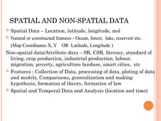
SPATIAL AND NON-SPATIAL DATA
PATIAL AND NON-SPATIAL DATA
 Spatial Data – Location, latitude, longitude, msl
 Natural or constructed features - Ocean, forest, lake, reservoir etc.
(Map Coordinates X, Y OR Latitude, Longitude )
Non-spatial data/Attribute data – SR, CSR, literacy, standard of
living, crop production, industrial production, labour,
migration, poverty, agriculture landuse, smart cities, etc
 Features : Collection of Data, processing of data, ploting of data
and models, Comparisons, generalization and making
hypothesis, formation of theory, formation of law
 Spatial and Temporal Data and Analysis (location and time)

8. DATA
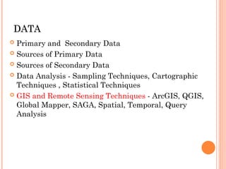
DATA
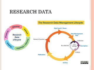
 Primary and Secondary Data
 Sources of Primary Data
 Sources of Secondary Data
 Data Analysis - Sampling Techniques, Cartographic
Techniques , Statistical Techniques
 GIS and Remote Sensing Techniques - ArcGIS, QGIS,
Global Mapper, SAGA, Spatial, Temporal, Query
Analysis

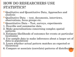
9. HOW DO RESEARCHERS USE
STATISTICS?
 Qualitative and Quantitative Data, Approaches and
analysis
 Qualitative Data – text, documents, interviews,
observations, focus groups etc.
 Quantitative Data – Test, surveys, experiments
1. Describe and summarize data
2. Make generalizations concerning complex spatial
patterns
3. Estimate likelihoods of outcomes for events at particular
location(s)
4. Use sample data to make inferences about a larger set of
data (a population)
5. Learn whether actual pattern matches an expected or
theoretical
6. Compare or associate (correlate) patterns of distributions

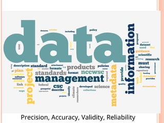
10. MEASUREMENT CONCEPTS
1.Precision- level of exactness associated with
measurement (rain gauge to inches or fractions of
inches)
2. Accuracy- extent of system wide bias in
measurement process
3. Validity- if geographical concept is complex
expressing “true” or “appropriate” meaning of the
concept through measurement may be difficult
(levels of poverty, economic well being,
environmental quality)
4. Reliability- changes in spatial patterns are
analyzed over time must ask about consistency
and stability of data

11. TYPES OF STATISTICAL
ANALYSIS
 Descriptive Statistics- concise numerical or
quantitative summaries of the characteristics of a
variable or data set (e.g. mean, standard deviation, etc).
 To present raw data ineffective/meaningful way using
numerical calculations or graphs or tables.
 This type of statistics is applied on already known data.
 To organize, analyze and present data in a meaningful
manner.
 It is used to describe a situation.

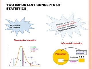
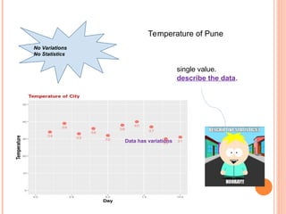
12. TWO IMPORTANT CONCEPTS OF
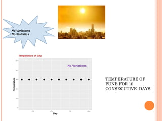
STATISTICS
No Variations
No Statistics
Descriptive statistics
Inferential statistics

13. No Variations
No Variations
No Statistics
TEMPERATURE OF
PUNE FOR 10
CONSECUTIVE DAYS.

14. Temperature of Pune
single value.
describe the data.
Data has variations
No Variations
No Statistics

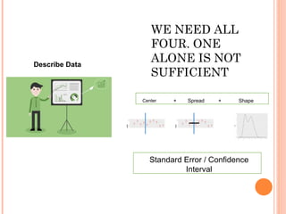
15. Describe Data
Center + Spread + Shape
WE NEED ALL
FOUR. ONE
ALONE IS NOT
SUFFICIENT
Standard Error / Confidence
Interval

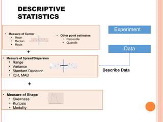
16. DESCRIPTIVE
STATISTICS
Experiment
Data
Describe Data
• Other point estimates
• Percentile
• Quantile
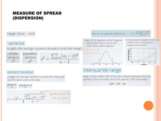
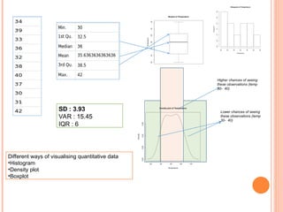
• Measure of Spread/Dispersion
• Range
• Variance
• Standard Deviation
• IQR, MAD
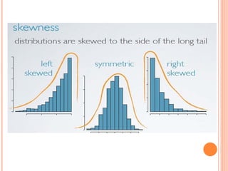
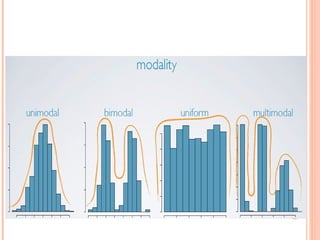
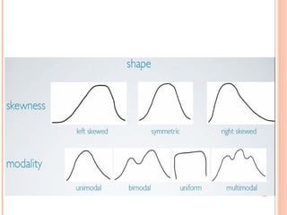
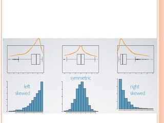
• Measure of Shape
• Skewness
• Kurtosis
• Modality
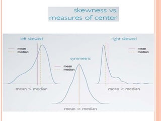
• Measure of Center
• Mean
• Median
• Mode
+
+

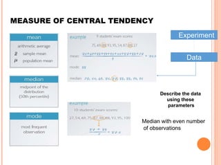
17. MEASURE OF CENTRAL TENDENCY
Experiment
Data
Describe the data
using these
parameters
Median with even number
of observations

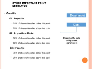
18. OTHER IMPORTANT POINT
ESTIMATES
Experiment
Data
Describe the data
using these
parameters
• Quartile
Q1 : 1st quartile
• 25% of observations lies below this point
• 75% of observations lies above this point
Q2 : 2nd quartile or Median
• 50% of observations lies below this point
• 50% of observations lies above this point
Q3 : 3rd quartile
• 75% of observations lies below this point
• 25% of observations lies above this point

19. MEASURE OF SPREAD
(DISPERSION)

20. Different ways of visualising quantitative data
•Histogram
•Density plot
•Boxplot
Higher chances of seeing
these observations (temp
30- 40)
Lower chances of seeing
these observations (temp
30- 40)
SD : 3.93
VAR : 15.45
IQR : 6

21. ROBUST STATISTICS FOR CENTRAL OR
SPREAD MEASURE

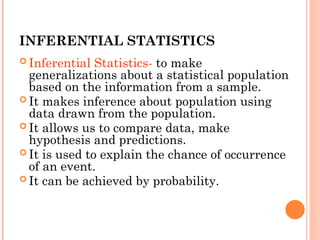
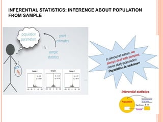
27. INFERENTIAL STATISTICS
 Inferential Statistics- to make
generalizations about a statistical population
based on the information from a sample.
 It makes inference about population using
data drawn from the population.
 It allows us to compare data, make
hypothesis and predictions.
 It is used to explain the chance of occurrence
of an event.
 It can be achieved by probability.

28. INFERENTIAL STATISTICS: INFERENCE ABOUT POPULATION
FROM SAMPLE

29. POINT
ESTIMATES

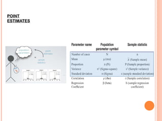
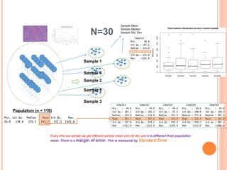
30. Population (n = 116)
Every time we sample we get different sample mean and std dev and it is different from population
mean. There is a margin of error. This is measured by Standard Error
Sample 1
Sample 4
Sample 2
Sample 5
Sample 3
N=30
Sample Mean
Sample Median
Sample Std. Dev

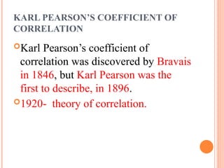
31. KARL PEARSON’S COEFFICIENT OF
CORRELATION
Karl Pearson’s coefficient of
correlation was discovered by Bravais
in 1846, but Karl Pearson was the
first to describe, in 1896.
1920- theory of correlation.

32. KARL PEARSON’S METHOD OF
PRODUCT MOMENTUM
 Denoted by r or rho.
 It is a measure of the degree of linear correlation between two
continuous variables.
Covariance of XY
r = ----------------------
(SDx *SDy)
Coefficient of Correlation or method of “Product momentum”.

33. PROPERTIES OF COEFFICIENT OF
CORRELATION
The Pearson correlation coefficients
can range in value from −1 to +1.
The Pearson correlation coefficient to
be +1, when one variable increases
then the other variable increases by a
consistent amount. This relationship
forms a perfect line.

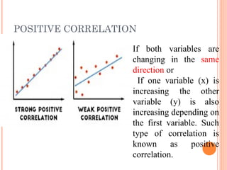
34. POSITIVE CORRELATION
If both variables are
changing in the same
direction or
If one variable (x) is
increasing the other
variable (y) is also
increasing depending on
the first variable. Such
type of correlation is
known as positive
correlation.

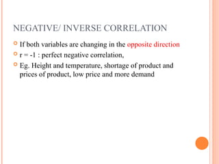
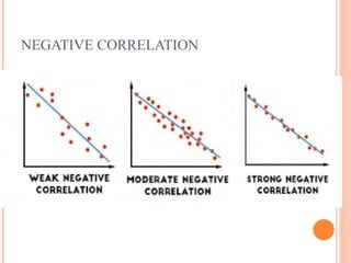
35. NEGATIVE/ INVERSE CORRELATION
 If both variables are changing in the opposite direction
 r = -1 : perfect negative correlation,
 Eg. Height and temperature, shortage of product and
prices of product, low price and more demand

36. NEGATIVE CORRELATION

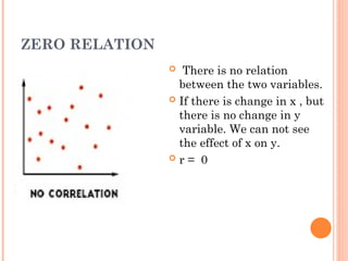
37. ZERO RELATION
 There is no relation
between the two variables.
 If there is change in x , but
there is no change in y
variable. We can not see
the effect of x on y.
 r = 0