Statistics And Probability Tutorial | Statistics And Probability for Data Science | Edureka

WHAT IS DATA?
CATEGORIES OF DATA
BASIC TERMINOLOGIES IN STATISTICS
SAMPLING TECHNIQUES
DESCRIPTIVE STATISTICS
TYPES OF STATISTICS
www.edureka.co/data-science
WHAT IS STATISTICS?
PROBABILITY
INFERENTIAL STATISTICS

WHAT IS DATA?

Data refers to facts and statistics collected together for reference or analysis.
Collected and Stored
Measured
Analyzed
Visualized
Data

CATEGORIES OF DATA

Types Of Data
Data
Qualitative Quantitative
Nominal Ordinal Discrete Continuous

Qualitative data deals with characteristics and descriptors that can't be easily measured, but
can be observed subjectively.
Nominal Data Ordinal Data
Data with no inherent order or ranking such as gender or race,
such kind of data is called Nominal data
Data with an ordered series, such as shown in the table, such
kind of data is called Ordinal data
Gender
Male
Female
Male
Male
Customer ID Rating
001 Good
002 Average
003 Average
004 Bad

Quantitative data deals with numbers and things you can measure objectively.
Discrete Data Continuous Data
Also known as categorical data, it can hold finite number of
possible values.
Data that can hold infinite number of possible values.
Example: Number of students in a class Example: Weight of a person

WHAT IS STATISTICS?

https://www.kaspersky.com/blog/tip-of-the-week-how-to-get-rid-of-unwanted-emails/3005/
WHAT IS STATISTICS?
Statistics is an area of applied mathematics concerned with the data
collection, analysis, interpretation and presentation.
Your company has created a new drug that may cure cancer.
How would you conduct a test to confirm the drug's
effectiveness?

WHAT IS STATISTICS?
You and a friend are at a baseball game, and out of the blue he
offers you a bet that neither team will hit a home run in that
game. Should you take the bet?

WHAT IS STATISTICS?
The latest sales data have just come in, and your boss wants
you to prepare a report for management on places where the
company could improve its business. What should you look
for? What should you not look for?

BASIC TERMINOLOGIES IN STATISTICS

Population: A collection or set of individuals or objects or events whose properties are to be analyzed.
Sample: A subset of population is called ‘Sample’. A well chosen sample will contain most of the information
about a particular population parameter
Statistics Terminologies
Population Sample

SAMPLING TECHNIQUES

Sampling
Probability Non-probability
Random Stratified Snowball Convenience
Systematic
Judgement
Quota

Random Sampling
Systematic Sampling
Stratified Sampling
Each member of the population has equal chance of being
selected in the sample.

Random Sampling
Systematic Sampling
Stratified Sampling
In Systematic sampling every nth record is chosen from the population to
be a part of the sample.
1 2 3
4 5 6
2 4 6
Everynthrecordischosen
Every2nd recordischosen

Random Sampling
Systematic Sampling
Stratified Sampling
• A stratum is a subset of the population that shares at least one common
characteristic, in this case it’s gender.
• Random sampling is used to select a sufficient number of subjects from
each stratum.
Malesubset
Femalesubset
Chosensample

TYPES OF STATISTICS

DESCRIPTIVE
STATISTICS
Descriptive statistics uses the data to provide descriptions of the
population, either through numerical calculations or graphs or tables.
Maximum
Average
Minimum
Descriptive Statistics is mainly focused upon the main characteristics of data. It
provides graphical summary of the data.

INFERENTIAL
STATISTICS
Inferential statistics makes inferences and predictions about a population based
on a sample of data taken from the population in question.
Large
Medium
Small
Inferential statistics, generalizes a large dataset and applies probability to draw a
conclusion. It allows us to infer data parameters based on a statistical model
using a sample data.

DESCRIPTIVE STATISTICS

Descriptive statistics is a method used to describe and understand the features of a specific data set by giving short summaries
about the sample and measures of the data.
Descriptive statistics is broken down into two categories:
• Measures of central tendency
• Measures of variability (spread)

Descriptive statistics are broken down into two categories:
• Measures of Central tendency
• Measures of Variability (spread)
Measures of Centre
Mean ModeMedian

Descriptive statistics are broken down into two categories:
• Measures of Central tendency
• Measures of Variability (spread)
Measures of Spread
Range Standard DeviationInter Quartile Range Variance

MEASURES OF CENTRE

Measure of average of all the values in a sample is called Mean.
Mean
Cars mpg cyl disp hp drat
MazdaRX4 21 6 160 110 3.9
MazdaRX4_
WAG 21 6 160 110 3.9
Datsun_710 22.8 4 108 93 3.85
Alto 21.3 6 108 96 3
WagonR 23 4 150 90 4
Toyata_ 11 23 6 108 110 3.9
Honda_12 23 4 160 110 3.9
Ford_11 23 6 160 110 3.9
Here is a sample dataset of cars containing the
variables:
• Cars,
• Mileage per Gallon(mpg)
• Cylinder Type (cyl)
• Displacement (disp)
• Horse Power(hp)
• Real Axle Ratio(drat)

To find out the average horsepower of the cars among the population of cars, we will check and calculate the
average of all values:
Mean
MazdaRX4 21 6 160 110 3.9
MazdaRX4_
WAG 21 6 160 110 3.9
Datsun_710 22.8 4 108 93 3.85
Alto 21.3 6 108 96 3
WagonR 23 4 150 90 4
Toyata_ 11 23 6 108 110 3.9
Honda_12 23 4 160 110 3.9
Ford_11 23 6 160 110 3.9
110 + 110 + 93 + 96 + 90 + 110 + 110 + 110
8
= 103.625
variables:
• Cars,
• Horse Power(hp)

Measure of the central value of the sample set is called Median.
Median
MazdaRX4 21 6 160 110 3.9
MazdaRX4_
WAG 21 6 160 110 3.9
Datsun_710 22.8 4 108 93 3.85
Alto 21.3 6 108 96 3
WagonR 23 4 150 90 4
Toyata_ 11 23 6 108 110 3.9
Honda_12 23 4 160 110 3.9
Ford_11 23 6 160 110 3.9
variables:
• Cars,
• Horse Power(hp)

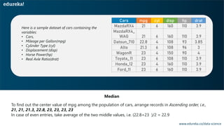
To find out the center value of mpg among the population of cars, arrange records in Ascending order, i.e.,
21, 21, 21.3, 22.8, 23, 23, 23, 23
In case of even entries, take average of the two middle values, i.e. (22.8+23 )/2 = 22.9
Median
MazdaRX4 21 6 160 110 3.9
MazdaRX4_
WAG 21 6 160 110 3.9
Datsun_710 22.8 4 108 93 3.85
Alto 21.3 6 108 96 3
WagonR 23 4 150 90 4
Toyata_ 11 23 6 108 110 3.9
Honda_12 23 4 160 110 3.9
Ford_11 23 6 160 110 3.9
variables:
• Cars,
• Horse Power(hp)

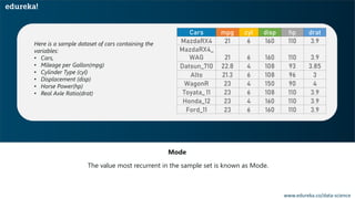
The value most recurrent in the sample set is known as Mode.
Mode
MazdaRX4 21 6 160 110 3.9
MazdaRX4_
WAG 21 6 160 110 3.9
Datsun_710 22.8 4 108 93 3.85
Alto 21.3 6 108 96 3
WagonR 23 4 150 90 4
Toyata_ 11 23 6 108 110 3.9
Honda_12 23 4 160 110 3.9
Ford_11 23 6 160 110 3.9
variables:
• Cars,
• Horse Power(hp)

To find the most common type of cylinder among the population of cars, check the value which is repeated
most number of times, i.e., cylinder type 6
Mode
MazdaRX4 21 6 160 110 3.9
MazdaRX4_
WAG 21 6 160 110 3.9
Datsun_710 22.8 4 108 93 3.85
Alto 21.3 6 108 96 3
WagonR 23 4 150 90 4
Toyata_ 11 23 6 108 110 3.9
Honda_12 23 4 160 110 3.9
Ford_11 23 6 160 110 3.9
variables:
• Cars,
• Horse Power(hp)

MEASURES OF SPREAD

A measure of spread, sometimes also called a measure of dispersion, is used to describe the variability in a
sample or population.
Range is the given measure of how spread apart the values in a dataset are.
Range = Max(𝑥𝑖) - Min(𝑥𝑖)

Quartiles tell us about the spread of a data set by breaking the data set into quarters, just like the
median breaks it in half.
1 2 3 4 5 6 7 8
Q1 Q2 Q3

Inter Quartile Range(IQR) is the measure of variability, based on dividing a dataset into quartiles.
• Quartiles divide a rank-ordered data set into four equal parts, denoted by Q1, Q2, and Q3,
respectively
• The interquartile range is equal to Q3 minus Q1, i.e.. IQR = Q3 - Q1

Variance describes how much a random variable differs from its expected value.
It entails computing squares of deviations.
x : Individual data points
n : Total number of data points
x̅ : Mean of data points

Deviation is the difference between each element from the mean.
Deviation = (𝑥𝑖-µ)

Population Variance is the average of squared deviations.
෍
𝑖=1
𝑁
= (𝑥𝑖−𝜇)²
1
𝑁
σ² =

Sample Variance is the average of squared differences from the mean.
෍
𝑖=1
𝑁
= (𝑥𝑖− ҧ𝑥)²
1
(𝑛 − 1)
s² =

Standard Deviation is the measure of the dispersion of a set of data from its mean.
𝜎 =
1
𝑁
෍
𝑖=1
𝑁
𝑥𝑖 − 𝜇 2

Standard Deviation Use Case: Daenerys has 20 Dragons. They have the numbers 9, 2, 5, 4, 12, 7, 8, 11, 9, 3, 7, 4, 12,
5, 4, 10, 9, 6, 9, 4. Work out the Standard Deviation.
Find out the
mean for your sample
set.
STEP 1
The Mean is:
9+2+5+4+12+7+8+11+9+3+7+4+12+5+4+10+9+6+9+4
20
⸫µ=7

Then for each number,
subtract the Mean and
square the result.
STEP 2
(𝑥𝑖−𝜇)²
(9-7)²= 2²=4
(2-7)²= (-5)²=25
(5-7)²= (-2)²=4
And so on…
⸫ We get the following results:
4, 25, 4, 9, 25, 0, 1, 16, 4, 16, 0, 9, 25, 4, 9, 9, 4, 1, 4, 9

Then work out the
mean of those squared
differences.
STEP 3
4+25+4+9+25+0+1+16+4+16+0+9+25+4+9+9+4+1+4+9
20
⸫ σ² = 8.9
෍
𝑖=1
𝑁
=(𝑥𝑖−𝜇)²
1
𝑁
σ =

Take square root of
σ².
STEP 4
⸫ σ = 2.983
෍
𝑖=1
𝑁
=(𝑥𝑖−𝜇)²
1
𝑁
σ =

INFORMATION GAIN & ENTROPY

Entropy Information Gain (IG)
Entropy measures the impurity or uncertainty present in the
data.
where:
• S – set of all instances in the dataset
• N – number of distinct class values
• pi – event probability
IG indicates how much “information” a particular feature/
variable gives us about the final outcome.
where:
H(S) – entropy of the whole dataset S
• |Sj| – number of instance with j value of an attribute A
• |S| – total number of instances in dataset S
• v – set of distinct values of an attribute A
• H(Sj) – entropy of subset of instances for attribute A
• H(A, S) – entropy of an attribute A

USE CASE

Forecast whether the match
will be played or not
according to weather
conditions

Outlook
Sunny Overcast Rain
Yes – 2
No – 3
Yes – 3
No – 2
Yes – 4
No – 0
Yes – 9
No – 5

From the total of 14 instances we have:
• 9 instances “yes”
• 5 instances “no”
The Entropy is:

Selecting the root variable

Information Gain of attribute “windy”
• 6 instances “true”
• 8 instances “false”

Information Gain of attribute “outlook”
• 5 instances “sunny”
• 4 instances “overcast”
• 5 instances “rainy”

Information Gain of attribute “humidity”
• 7 instances “high”
• 7 instances “normal”

Information Gain of attribute “temperature”
• 4 instances “hot”
• 6 instances “mild”
• 4 instances “cool”

The variable with the highest IG is used to split the data at the root node.
Gain = 0.247 Gain = 0.048 Gain = 0.151 Gain = 0.029

Gain = 0.247 Gain = 0.048 Gain = 0.151 Gain = 0.029
The variable with the highest IG is used to split the data at the root node. The ‘Outlook’ variable has the highest IG, therefore
it can be assigned to the root node.

CONFUSION MATRIX

A confusion matrix is a table that is often used to describe the performance of a classification model (or "classifier")
on a set of test data for which the true values are known.
Confusion Matrix represents a tabular representation of Actual vs Predicted values
You can calculate the accuracy of your model with:

• There are two possible predicted classes: "yes" and "no”
• The classifier made a total of 165 predictions
• Out of those 165 cases, the classifier predicted "yes" 110 times, and "no" 55 times
• In reality, 105 patients in the sample have the disease, and 60 patients do not

PROBABILITY

• Probability is the ratio of desired outcomes to total outcomes:
(desired outcomes) / (total outcomes)
• Probabilities of all outcomes always sums to 1
Example:
• On rolling a dice, you get 6 possible outcomes
• Each possibility only has one outcome, so each has a probability of 1/6
• For example, the probability of getting a number ‘2’ on the dice is 1/6
Probability is the measure of how likely an event will occur.

TERMINOLOGIES IN PROBABILITY

Disjoint Events do not have any common outcomes.
• The outcome of a ball delivered cannot be a sixer and a wicket
• A single card drawn from a deck cannot be a king and a queen
• A man cannot be dead and alive
Non-Disjoint Events can have common outcomes
• A student can get 100 marks in statistics and 100 marks in probability
• The outcome of a ball delivered can be a no ball and a six

PROBABILITY DISTRIBUTION

Graph of a PDF will be continuous over a range
Area bounded by the curve of density function
and the x-axis is equal to 1
Probability that a random variable assumes a
value between a & b is equal to the area under
the PDF bounded by a & b
The equation describing a continuous probability distribution is called a Probability Density Function
a b

The Normal Distribution is a probability distribution that associates the normal random variable X with a
cumulative probability
Y = [ 1/σ * sqrt(2π) ] * e -(x - μ)2/2σ2
Where,
•X is a normal random variable
•μ is the mean and
•σ is the standard deviation
Note: Normal Random variable is variable with mean at 0 and variance equal to 1

The graph of the Normal Distribution depends on two factors: the Mean and the Standard Deviation
• Mean: Determines the location of center of the graph
• Standard Deviation: Determines the height of the graph
If the standard deviation is large,
the curve is short and wide.
If the standard deviation is small, the
curve is tall and narrow.

The Central Limit Theorem states that the sampling distribution of the mean of any independent,
random variable will be normal or nearly normal, if the sample size is large enough

TYPES OF PROBABILITY

Marginal Probability is the probability of occurrence of a single event.
Marginal Probability = 13
52
It can be expressed as: P (A) = σ𝑖=1
𝑘
𝑃( 𝑥𝑖 )

Joint Probability is a measure of two events happening at the same time
Example: The probability that a card is an Ace of hearts = P (Ace of hearts)
(There are 13 heart cards in a deck of 52 and out of them one in the Ace of hearts)

• Probability of an event or outcome based on the occurrence of a previous event or outcome
• Conditional Probability of an event B is the probability that the event will occur given that an event A has
already occurred
If A and B are dependent events then the
expression for conditional probability is given by:
P (B|A) = P (A and B) / P (A)
If A and B are independent events then the
expression for conditional probability is given by:
P(B|A) = P (B)

Finding the probability that a candidate has undergone Edureka’s training

The probability that a candidate has undergone Edureka’s training
P(Edu.Training ) = 45 /105 ≈ 0.42

Finding the probability that a candidate has attended Edureka’s training and also has good package.

P (Good Package & Edu.Training ) =
30 /105 ≈ 0.28
Salary Training

Finding the probability that a candidate has a good package given that he has not undergone training

P (Good Package | Without Edureka) = 5 / 60 ≈ 0.08

BAYES’ THEOREM

Shows the relation between one conditional probability and its inverse
P (B|A) is referred to as likelihood ratio which
measures the probability (given event A) of
occurrence of B
P (A) is referred to as Prior which
represents the actual probability
distribution of A
P (A|B) = P (B|A) P (A) P (B)
P (A|B) is referred to as posterior which
means the probability of occurrence of A
given B

“ Consider 3 bowls. Bowl A contains 2 blue balls and 4 red balls; Bowl B contains 8 blue balls and 4 red balls,
Bowl C contains 1 blue ball and 3 red balls. We draw 1 ball from each bowl. What is the probability to draw a
blue ball from Bowl A if we know that we drew exactly a total of 2 blue balls? ”
Bowl A Bowl B Bowl C

• Let A be the event of picking a blue ball from bag A, and let X be the event of picking exactly
two blue balls
• We want Probability(A∣X), i.e. probability of occurrence of event A given X
By the definition of Conditional Probability,
• We need to find the two probabilities on the right-side of equal to symbolop
P𝑟 𝐴 𝑋 = 𝑃𝑟 (𝐴 ∩ X)
Pr (X)

Steps to execute the problem
First find Pr(X). This can happen in three ways:
(i) white from A, white from B, red from C
(ii) white from A, red from B, white from C
(iii) red from A, white from B, white from C
Next we find Pr(A∩X).
This is the sum of terms (i) and (ii) above
Step 1:
Step 2:

INFERENTIAL STATISTICS

POINT ESTIMATION

Point Estimation is concerned with the use of the sample data to measure a single value which serves as an
approximate value or the best estimate of an unknown population parameter.
Population Sample
Random
Estimate
ҧ𝑥𝜇
Mean of
Population
Sample Mean
Point Estimation is concerned with the use of the sample data to measure a single value which serves as an
approximate value or the best estimate of an unknown population parameter.

Method of Moments
Estimates are found out by equating the first k sample
moments to the corresponding k population moments
Maximum of Likelihood
Uses a model and the values in the model to maximize a
likelihood function. This results in the most likely
parameter for the inputs selected
Bayes’ Estimators
Minimizes the average risk (an expectation of random
variables)
Best Unbiased Estimators
Several unbiased estimators can be used to approximate a
parameter (which one is “best” depends on what parameter
you are trying to find)

There are two important
statistical parameters to
determine how well the point
estimates generalise the entire
population. Let’s explore them
too

INTERVAL ESTIMATION

An Interval, or range of values, used to estimate a population parameter is called Interval Estimate.

03
01
02
Confidence Interval is the measure of your confidence, that the interval
estimate contains the population mean, 𝜇
Statisticians use a confidence interval to describe the amount of uncertainty
associated with a sample estimate of a population parameter
Technically, a range of values so constructed that there is a specified probability
of including the true value of a parameter within it

• Difference between the point estimate and the actual population parameter value is called the Sampling Error
• When 𝜇 is estimated, the sampling error is the difference 𝜇 - ҧ𝑥
Margin of Error E, for a given level of confidence is the greatest possible distance between the
point estimate and the value of the parameter it is estimating

ESTIMATING LEVEL OF CONFIDENCE

The level of confidence c, is the probability that the interval estimate contains the population parameter.
C is the area beneath the normal curve between the critical values
Corresponding Z score can be calculated using the standard normal table

If the level of confidence is 90%, this means that you are 90% confident that the interval contains
the population mean, 𝜇.
The Corresponding Z – scores are ± 1.645

A random sample of 32 textbook prices is taken from a local college bookstore. The mean of the sample is 𝑥 ̅ = 74.22, and
the sample standard deviation is S = 23.44. Use a 95% confidence level and find the margin of error for the mean price of all
textbooks in the bookstore

You know by formula,
E = 1.96 * (23.44/√32) ≈ 8.12
A random sample of 32 textbook prices is taken from a local college bookstore. The mean of the sample is 𝑥 ̅ = 74.22, and
the sample standard deviation is S = 23.44. Use a 95% confidence level and find the margin of error for the mean price of all
textbooks in the bookstore

HYPOTHESIS TESTING

Statisticians use hypothesis testing to formally check whether the hypothesis is
accepted or rejected.
Hypothesis testing is conducted in the following manner:
❖ State the Hypotheses – This stage involves stating the null and alternative hypotheses.
❖ Formulate an Analysis Plan – This stage involves the construction of an analysis plan.
❖ Analyse Sample Data – This stage involves the calculation and interpretation of the test statistic as
described in the analysis plan.
❖ Interpret Results – This stage involves the application of the decision rule described in the analysis plan.

UNDERSTANDING HYPOTHESIS TESTING

Nick John Bob Harry
Assume the event is free of bias.
So, what is the probability of John not cheating?

P(John not picked for a day) =
3
4
P(John not picked for 3 days) =
3
4
×
3
4
×
3
4
= 0.42 (approx)
P(John not picked for 12 days) = (
3
4
) 12 = 0.032 < 𝟎. 𝟎𝟓
Nick John Bob Harry

Null Hypothesis (𝑯 𝟎) : Result is no different from assumption.
Alternate Hypothesis (𝑯 𝒂) : Result disproves the assumption.
Probability of Event < 𝟎. 𝟎𝟓 (5%)
Nick John Bob Harry

Statistics And Probability Tutorial | Statistics And Probability for Data Science | Edureka

Statistics And Probability Tutorial | Statistics And Probability for Data Science | Edureka

More Related Content

What's hot

Similar to Statistics And Probability Tutorial | Statistics And Probability for Data Science | Edureka

More from Edureka!

Recently uploaded

Statistics And Probability Tutorial | Statistics And Probability for Data Science | Edureka