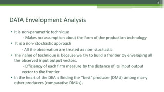
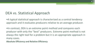
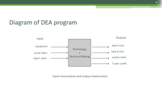
DEA is a non-parametric technique used to measure the relative efficiency of decision making units (DMUs) that use multiple inputs to produce multiple outputs. It works by constructing a production frontier boundary comprised of the most efficient DMUs to evaluate how efficiently other DMUs use inputs to produce outputs. The methodology was originally developed in 1978 and has since been applied in various industries to evaluate organizations, identify best practices, and determine potential efficiency improvements for inefficient units.

1. Data Envelopment Analysis
Presented by
Prashant Chouhan (172TS016)

2. Content
• Introduction to Data Envelopment Analysis (DEA)
• History and Development
• What does DEA do?
• DEA vs. Statistical Approach
• Graphical Depiction of DEA
• Data envelopment analysis (DEA) Methodology
• DEA Algorithm and Model
• Limitations of DEA
2

3. Introduction to DEA
Data Envelopment Analysis (DEA) is a very powerful service management
and benchmarking technique originally developed by Chames, Cooper
and Rhodes (1978) to evaluate nonprofit and publicsector organizations
Data Envelopment Analysis (DEA) is a linear programming methodology to
measure the efficiency of multiple decision-making units (DMU) when the
production process presents a structure of multiple inputs and outputs.
3

4. DATA Envelopment Analysis
• It is non-parametric technique
- Makes no assumption about the form of the production technology
• It is a non- stochastic approach
- All the observation are treated as non- stochastic
• The name of technique is because we try to build a frontier by enveloping all
the observed input output vectors.
- Efficiency of each firm measure by the distance of its input output
vector to the frontier
• In the heart of the DEA is finding the "best" producer (DMU) among many
other producers (comparative DMUs).
4

5. History and Development
• The first application of DEA was in the agriculture field, by Farrell in
1957
• Mathematical programming technique presented in 1978 by Charnes et
al.
• Since then it has been used to assess efficiency in areas such as health
(Wilson et al. 2012).
• Nowadays DEA can be seen to have spread to other fields such as transit
,mining, air transportation and even banking.
5

6. What does DEA do?
1. DEA compares service units considering all resources used and
services provided, and identifies the most efficient units and the
inefficient units in which real efficiency improvements are possible.
2. DEA calculates the amount and type of cost and resource savings that
can be achieved by making each inefficient unit as efficient as the
most efficient – best practice units.
6

7. What does DEA do?
3. Specific changes in the inefficient service units are identified. These
changes would make the efficient units performance approach the
best practice unit performance.
4. Management receives information about performance of service units
that can be used to help transfer system and managerial expertise
from better-managed, relatively efficient units to the inefficient ones.
This has resulted in improving the productivity of the inefficient units,
reducing operating costs and increasing profitability.
7

8. DEA vs. Statistical Approach
•A typical statistical approach is characterized as a central tendency
approach and it evaluates producers relative to an average producer.
•In contrast, DEA is an extreme point method and compares each
producer with only the "best" producers. Extreme point method is not
always the right tool for a problem but it is an appropriate approach in
many cases.
Absolute Efficiency and Relative Efficiency
8

9. Diagram of DEA program
Technology
+
Decision Making
Outputs
equipment
server labor
mgmt. labor
type A cost.
type B cost.
quality index
$ oper. profit
Input minimisation and output maximisation
Input
9

10. Graphical Depiction of DEA
• Frontier defines the (observed) efficient trade-
off among inputs and outputs within a set of
DMUs.
• Relative distance to the frontier defines
efficiency
• “Nearest point” on frontier defines an efficient
comparison unit (hypothetical comparison
unit (HCU))
• Differences in inputs and output between
DMU and HCU define productivity “gaps”
(improvement potential)
Efficiency of B =OB/OB1
10
o

11. Data envelopment analysis (DEA) Methodology
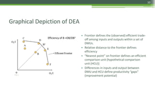
• DEA requires the multiple inputs and outputs for each DMU to be
specified.
• DEA defines efficiency score for each DMU as a weighted sum of
outputs [total output] divided by a weighted sum of inputs [total input].
• DEA restricts all efficiency scores to the range 0 to 1.
• DEA calculates the numerical value of the efficiency score for a
particular DMU by choosing input/output weights that maximize the
score, thereby presenting the DMU in the best possible light.
11

12. DEA Algorithm
• First Step: Selection of the Homogeneous DMUs
• Second Step: Selection of Input and Output Variables
Input
1. Fleet size (FS),
2. Total Staff (TS),
3. Fuel consumption (FC)
4. Accident per lakh kilometers (APLK)
output
1. Bus Utilisation (BU),
2. Passenger kilometers
3. Load Factor (LF)
12

13. Third step : Selection of the model
• CCR Model (Primal and Dual)
• BCC Model
• Super Efficiency Model
• DEA Models with Weight Restrictions
• Cross-Efficiency Models in DEA
• Benchmarking in DEA
• DEA Windows Analysis
• DEA with Ordinal and Cardinal Factors
13

14. CCR : Primal Form
jkuv
i
xu
yv
ts
xu
yv
jk
m
j
jij
ki
s
k
k
m
j
jpj
kp
s
k
k
,0,
,1.
max
1
1
1
1










jkuv
ixuyv
xuts
yv
jk
m
j
jijki
s
k
k
m
j
jpj
kp
s
k
k
,0,
,0
1.
max
11
1
1









where: p is the unit being evaluated; s represents the number of outputs; m represents the
number of inputs; yki is the amount of output k provided by unit i; xji is the amount of
input j used by unit i; vk and uj are the weights given to output k and input j, respectively.
14

15. BCC Model
• BCC model given by Banker, Charnes and Cooper.
• The primary difference between BCC model and CCR model is the
convexity constraint, which represents the returns to scale.
• Returns to scale reflects the extent to which a proportional increase in
all inputs increases outputs.
• In the BCC model λjk ’s are now restricted to 𝐣=𝟏
𝐧
𝛌𝐣𝐤=1 which is known
as convexity constraint. Technical efficiency assessed by BCC model is
pure technical efficiency.
15

16. Super Efficiency Model
jkuv
pixuyv
xuts
yv
jk
m
j
jijki
s
k
k
m
j
jpj
kp
s
k
k
,0,
,0
1.
max
11
1
1









The DMU being evaluated
is removed from the constraint
set thereby allowing its efficiency
score to exceed a value of 1.00
It can be used to evaluate efficient units
directly. It means without solving the
CCR model, one can rank efficient
DMUs by solving just the super-
efficiency model.
16

17. DEA Models with Weight Restrictions
• One of the drawbacks of this method is optimization becoming
extremely weighted referring to advantaged inputs or outputs becoming
more disadvantaged in terms of DMUs ranking. Since yielding many
numbers of DMUs as efficient.
• Weight restriction using coefficient of variation of inputs and outputs
for a nonlinear optimization model.
• Methods such as AHP and ANP can be utilized for identifying weight
restriction constraints in DEA.
17

18. Fourth step : Calculating the overall technical efficiency (OTE)
𝑟=1
𝑠
𝑢 𝑟 𝑦𝑟𝑜
𝑖=1
𝑠
𝑣𝑖 𝑥𝑖𝑜
Weights.
Selected input
of each facility
in the set o.
Selected output
of each facility
in the set o.
Maximize Eo =
Objective
Efficiency score
18

19. Fifth Step: Calculating the pure technical efficiency (PTE) and scale
efficiency (SE) of STU:.
• Technical efficiency assessed by BCC model is pure technical efficiency
because it has net of any scale effect.
• Scale efficiency of Kth DMU = Overall Technical Efficiency of the kth DMU
Pure Technical Efficiency of the kth DMU
19

20. Limitations of DEA
• DEA is good at estimating "relative" efficiency of a DMU but it converges
very slowly to "absolute" efficiency.
• DEA can tell how well you are doing compared to your peers but not
compared to a "theoretical maximum."
• Since a standard formulation of DEA creates a separate linear program
for each DMU, large problems can be computationally intensive.
• The number of efficient firms on the frontier tends to increase with the
number of inputs and output variables
20

21. Reference
• nptel.ac.in
• www.springer.com
• www.researchgate.net
• arxiv.org
• www.sciencedirect.com
21

22. 22