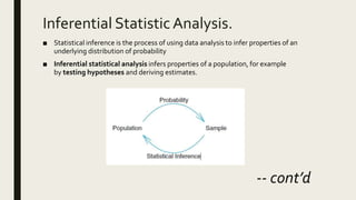
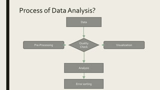
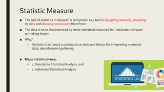
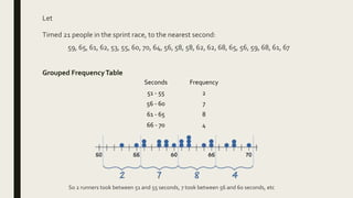
1) The document discusses data analysis and provides definitions and explanations of key concepts in data analysis such as descriptive statistical analysis, measures of central tendency, frequency distribution, and inferential statistical analysis.
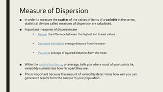
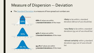
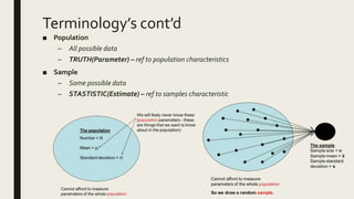
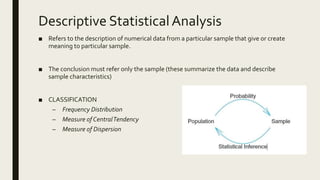
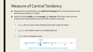
2) It explains that descriptive statistical analysis describes and summarizes sample data through measures like frequency distribution, measures of central tendency, and measures of dispersion.
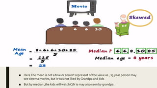
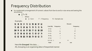
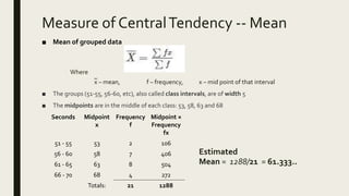
3) Frequency distribution involves grouping numeric data into intervals and counting the frequency of values within each interval. Measures of central tendency like the mean, median, and mode provide a single value to represent the center of a data set.

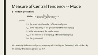
![Measure of CentralTendency -- Mode
L = 60.5
fm-1 = 7
fm = 8
fm+1 = 4
w = 5
– Estimated Mode= 60.5 + [8 − 7 / (8 − 7) + (8 − 4) ]× 5
= 60.5 + (1/5) × 5
= 61.5
final result is:
• Estimated Mean: 61.333...
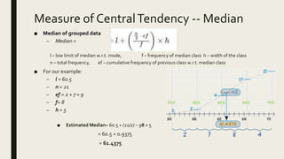
• Estimated Median: 61.4375
• Estimated Mode: 61.5 0
10
20
30
40
50
60
70
80
1 2 3 4 5 6 7 8 9 10 11 12 13 14 15 16 17 18 19 20 21
0
1
2
3
4
5
6
7
8
9
51 - 55 56 - 60 61 - 65 66 - 70](https://image.slidesharecdn.com/dataanalysis-220327140249/85/Data-Analysis-pptx-21-320.jpg)