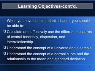
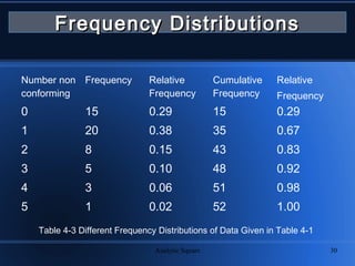
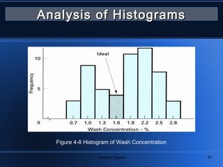
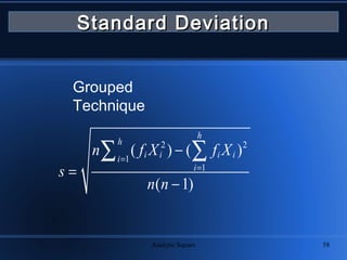
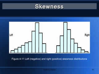
The document outlines the fundamentals of statistics, covering important topics such as measures of central tendency, dispersion, frequency distributions, and significant figures. It defines statistics and distinguishes between descriptive and inferential statistics, while explaining different types of data and their analysis methods. Additionally, it explains how to construct histograms and various statistical measures, including accuracy, precision, skewness, and kurtosis.

1. Analytic Square 1
Fundamentals ofFundamentals of
StatisticsStatistics
Analytic SquareAnalytic Square
Making the DifferenceMaking the Difference

2. Analytic Square 2
Outline
 Introduction
 Frequency Distribution
 Measures of Central Tendency
 Measures of Dispersion

3. Analytic Square 3
Outline-Continued
 Other Measures
 Concept of a Population and Sample
 The Normal Curve
 Tests for Normality

4. Analytic Square 4
Learning Objectives
When you have completed this chapter you
should be able to:
 Know the difference between a variable and an
attribute.
 Perform mathematical calculations to the correct
number of significant figures.
 Construct histograms for simple and complex
data.

5. Analytic Square 5
Learning Objectives-cont’d.
When you have completed this chapter you should
be able to:
 Calculate and effectively use the different measures
of central tendency, dispersion, and
interrelationship.
 Understand the concept of a universe and a sample.
 Understand the concept of a normal curve and the
relationship to the mean and standard deviation.

6. Analytic Square 6
Learning Objectives-cont’d.
When you have completed this chapter you should be
able to:
 Calculate the percent of items below a value, above a
value, or between two values for data that are normally
distributed.
 Calculate the process center given the percent of items
below a value
 Perform the different tests of normality
 Construct a scatter diagram and perform the necessary
related calculations.

7. Analytic Square 7
Definition of Statistics:
1. A collection of quantitative data pertaining to a
subject or group. Examples are blood
pressure statistics etc.
2. The science that deals with the collection,
tabulation, analysis, interpretation, and
presentation of quantitative data
IntroductionIntroduction

8. Analytic Square 8
Two phases of statistics:
 Descriptive Statistics:
Describes the characteristics of a product or
process using information collected on it.
 Inferential Statistics (Inductive):
Draws conclusions on unknown process
parameters based on information contained in a
sample.
Uses probability
IntroductionIntroduction

9. Analytic Square 9
Types of Data:
Attribute:
Discrete data. Data values can only be integers.
Counted data or attribute data. Examples include:
 How many of the products are defective?
 How often are the machines repaired?
 How many people are absent each day?
Collection of DataCollection of Data

10. Analytic Square 10
Types of Data:
Attribute:
Discrete data. Data values can only be
integers. Counted data or attribute data.
Examples include:
 How many days did it rain last month?
 What kind of performance was achieved?
 Number of defects, defectives
Collection of Data – Cont’d.Collection of Data – Cont’d.

11. Analytic Square 11
Types of Data:
Variable:
Continuous data. Data values can be any real
number. Measured data.
Examples include:
 How long is each item?
 How long did it take to complete the task?
 What is the weight of the product?
 Length, volume, time
Collection of DataCollection of Data

12. Analytic Square 12
Collection of DataCollection of Data
 Significant Figures
 Rounding

13. Analytic Square 13
 Significant Figures = Measured numbers
 When you measure something there is always
room for a little bit of error
 How tall are you 5 ft 9 inches or 5 ft 9.1 inches?
 Counted numbers and defined numbers ( 12 ins.
= 1 ft, there are 6 people in my family)
Significant FiguresSignificant Figures

14. Analytic Square 14
 Significant figures are used to indicate the amount of
variation which is allowed in a number.
 It is believed to be closer to the actual value than any
other digit.
 Significant figures:
 3.69 – 3 significant digits.
 36.900 – 5 significant digits.
Significant FiguresSignificant Figures

15. Analytic Square 15
 Use Scientific Notation
 3x10^2 (1 significant digit)
 3.0x10^2 (2 significant digits)
Significant Figures – Cont’d.Significant Figures – Cont’d.

16. Analytic Square 16
 Rules for Multiplying and Dividing
 Number of sig. = the same as the number with the
least number of significant digits.
 6.59 x 2.3 = 15
 32.65/24 = 1.4 (where 24 is not a counting
number)
 32.64/24=1.360(24 is a counting number i.e.
24.00)
Significant FiguresSignificant Figures

17. Analytic Square 17
Rules for Adding and Subtracting
 Result can have no more sig. fig. after the decimal
point than the number with the fewest sig. fig. after the
decimal point.
 38.26 – 6 = 32 (6 is not a counting number)
 38.2 -6 = 32.2 (6 is a counting number)
 38.26 – 6.1 = 32.2 (rounded from 32.16)
 If the last digit >=5 then round up, else round down
Significant FiguresSignificant Figures

18. Analytic Square 18
Precision
The precision of a measurement is determined by
how reproducible that measurement value is.
For example if a sample is weighed by a student
to be 42.58 g, and then measured by another
student five different times with the resulting data:
42.09 g, 42.15 g, 42.1 g, 42.16 g, 42.12 g Then
the original measurement is not very precise
since it cannot be reproduced.
Precision and AccuracyPrecision and Accuracy

19. Analytic Square 19
Accuracy
 The accuracy of a measurement is determined by how
close a measured value is to its “true” value.
 For example, if a sample is known to weigh 3.182 g, then
weighed five different times by a student with the resulting
data: 3.200 g, 3.180 g, 3.152 g, 3.168 g, 3.189 g
 The most accurate measurement would be 3.180 g,
because it is closest to the true “weight” of the sample.
Precision and AccuracyPrecision and Accuracy

20. Analytic Square 20
Precision and AccuracyPrecision and Accuracy
Figure 4-1 Difference between accuracy and precision

21. Analytic Square 21
 Frequency Distribution
 Measures of Central Tendency
 Measures of Dispersion
DescribingDescribing DataData

22. Analytic Square 22
 Ungrouped Data
 Grouped Data
Frequency DistributionFrequency Distribution

23. Analytic Square 23
2-72-7
There are three types of frequency
distributions
 Categorical frequency distributions
 Ungrouped frequency distributions
 Grouped frequency distributions
Frequency DistributionFrequency Distribution

24. Analytic Square 24
2-72-7
Categorical frequency distributions
 Can be used for data that can be placed in
specific categories, such as nominal- or
ordinal-level data.
 Examples - political affiliation, religious
affiliation, blood type etc.
CategoricalCategorical

25. Analytic Square 25
2-82-8
Example :Blood Type Frequency
Distribution
Class Frequency Percent
A 5 20
B 7 28
O 9 36
AB 4 16
CategoricalCategorical

26. Analytic Square 26
2-92-9
Ungrouped frequency distributions
 Ungrouped frequency distributions - can be
used for data that can be enumerated and
when the range of values in the data set is
not large.
 Examples - number of miles your instructors
have to travel from home to campus, number
of girls in a 4-child family etc.
UngroupedUngrouped

27. Analytic Square 27
2-102-10
Example :Number of Miles Traveled
Class Frequency
5 24
10 16
15 10
UngroupedUngrouped

28. Analytic Square 28
2-112-11
 Grouped frequency distributions
 Can be used when the range of values in
the data set is very large. The data must be
grouped into classes that are more than one
unit in width.
 Examples - the life of boat batteries in
hours.
GroupedGrouped

29. Analytic Square 29
2-122-12
Example: Lifetimes of Boat Batteries
Class
limits
Class
Boundaries
Cumulative
24 - 30 23.5 - 37.5 4 4
38 - 51 37.5 - 51.5 14 18
52 - 65 51.5 - 65.5 7 25
frequency
Frequency
GroupedGrouped

30. Analytic Square 30
Number non
conforming
Frequency Relative
Frequency
Cumulative
Frequency
Relative
Frequency
0 15 0.29 15 0.29
1 20 0.38 35 0.67
2 8 0.15 43 0.83
3 5 0.10 48 0.92
4 3 0.06 51 0.98
5 1 0.02 52 1.00
Table 4-3 Different Frequency Distributions of Data Given in Table 4-1
Frequency DistributionsFrequency Distributions

31. Analytic Square 31
Frequency Histogram
0
5
10
15
20
25
0 1 2 3 4 5
Number Nonconforming
Frequency
Frequency HistogramFrequency Histogram

32. Analytic Square 32
Relative Frequency Histogram
0.00
0.05
0.10
0.15
0.20
0.25
0.30
0.35
0.40
0.45
0 1 2 3 4 5
Number Nonconforming
RelativeFrequency
Relative Frequency HistogramRelative Frequency Histogram

33. Analytic Square 33
Cumulative Frequency Histogram
0
10
20
30
40
50
60
0 1 2 3 4 5
Number Nonconforming
CumulativeFrequency
Cumulative FrequencyCumulative Frequency
HistogramHistogram

34. Analytic Square 34
The histogram is the most important graphical tool
for exploring the shape of data distributions.
Check:
http://quarknet.fnal.gov/toolkits/ati/histograms.html
for the construction ,analysis and understanding of
histograms
The HistogramThe Histogram

35. Analytic Square 35
The Fast Way
Step 1: Find range of distribution, largest -
smallest values
Step 2: Choose number of classes, 5 to 20
Step 3: Determine width of classes, one
decimal place more than the data, class width =
range/number of classes
Step 4: Determine class boundaries
Step 5: Draw frequency histogram
#classes n=
Constructing a HistogramConstructing a Histogram

36. Analytic Square 36
Number of groups or cells
 If no. of observations < 100 – 5 to 9 cells
 Between 100-500 – 8 to 17 cells
 Greater than 500 – 15 to 20 cells
Constructing a HistogramConstructing a Histogram

37. Analytic Square 37
For a more accurate way of drawing a
histogram see the section on grouped data
in your textbook
Constructing a HistogramConstructing a Histogram

38. Analytic Square 38
 Bar Graph
 Polygon of Data
 Cumulative Frequency Distribution or Ogive
Other Types ofOther Types of
Frequency Distribution GraphsFrequency Distribution Graphs

39. Analytic Square 39
Bar Graph and Polygon of DataBar Graph and Polygon of Data

40. Analytic Square 40
Cumulative FrequencyCumulative Frequency

41. Analytic Square 41Figure 4-6 Characteristics of frequency distributions
Characteristics of FrequencyCharacteristics of Frequency
Distribution GraphsDistribution Graphs

42. Analytic Square 42
Analysis of HistogramsAnalysis of Histograms
Figure 4-7 Differences due to location, spread, and shape

43. Analytic Square 43
Analysis of HistogramsAnalysis of Histograms
Figure 4-8 Histogram of Wash Concentration

44. Analytic Square 44
The three measures in common use are the:
 Average
 Median
 Mode
Measures of Central TendencyMeasures of Central Tendency

45. Analytic Square 45
There are three different techniques
available for calculating the average three
measures in common use are the:
 Ungrouped data
 Grouped data
 Weighted average
AverageAverage

46. Analytic Square 46
1
n
i
i
X
X
n=
= ∑
Average-Ungrouped DataAverage-Ungrouped Data

47. Analytic Square 47
1
1 1 2 2
1 2
... .
...
h
i i
i
h h
h
f X
X
n
f X f X f X
f f f
=
=
+ +
=
+ +
∑
h = number of cellsh = number of cells fi=frequencyfi=frequency
Xi=midpointXi=midpoint
Average-Grouped DataAverage-Grouped Data

48. Analytic Square 48
1
1
n
i ii
w n
i
i
w X
X
w
=
=
=
∑
∑
Used when a number of averages are
combined with different frequencies
Average-Weighted AverageAverage-Weighted Average

49. Analytic Square 49
2
m
d m
m
n
cf
M L i
f
 
− 
= + 
 
 
Lm=lower boundary of the cell with the median
N=total number of observations
Cfm=cumulative frequency of all cells below m
Fm=frequency of median cell
i=cell interval
Median-Grouped DataMedian-Grouped Data

50. Analytic Square 50
Boundaries Midpoint Frequency Computation
23.6-26.5 25.0 4 100
26.6-29.5 28.0 36 1008
29.6-32.5 31.0 51 1581
32.6-35.5 34.0 63 2142
35.6-38.5 37.0 58 2146
38.6-41.5 40.0 52 2080
41.6-44.5 43.0 34 1462
44.6-47.5 46.0 16 736
47.6-50.5 49.0 6 294
Total 320 11549
Table 4-7 Frequency Distribution of the Life of 320 tires in 1000 km
Example ProblemExample Problem

51. Analytic Square 51
2
m
d m
m
n
cf
M L i
f
 
− 
= + 
 
 
320
154
235.6 3 35.9
58
Md
 
− 
= + = 
 
 
Median-Grouped DataMedian-Grouped Data
Using data from Table 4-7

52. Analytic Square 52
ModeMode
The Mode is the value that occurs with the
greatest frequency.
It is possible to have no modes in a series or
numbers or to have more than one mode.

53. Analytic Square 53Figure 4-9 Relationship among average, median and mode
Relationship Among theRelationship Among the
Measures of Central TendencyMeasures of Central Tendency

54. Analytic Square 54
 Range
 Standard Deviation
 Variance
Measures of DispersionMeasures of Dispersion

55. Analytic Square 55
The range is the simplest and easiest to
calculate of the measures of dispersion.
Range = R = Xh - Xl
 Largest value - Smallest value in
data set
MeasuresMeasures of Dispersion-Rangeof Dispersion-Range

56. Analytic Square 56
Sample Standard Deviation:
2
1
( )
1
n
i
Xi X
S
n
=
−
=
−
∑
2
2
1
1
/
1
n
n
i
i
Xi Xi n
S
n
=
=
 
− ÷
 =
−
∑ ∑
Measures of Dispersion-Measures of Dispersion-
Standard DeviationStandard Deviation

57. Analytic Square 57
Ungrouped Technique
2 2
1 1
( )
( 1)
n n
i i
n Xi Xi
S
n n
= =
−
=
−
∑ ∑
Standard DeviationStandard Deviation

58. Analytic Square 58
2 2
1
1
( ) ( )
( 1)
h
h
i i i ii
i
n f X f X
s
n n
=
=
−
=
−
∑ ∑
Standard DeviationStandard Deviation
Grouped
Technique

59. Analytic Square 59
Relationship Between theRelationship Between the
Measures of DispersionMeasures of Dispersion
 As n increases, accuracy of R decreases
 Use R when there is small amount of data or data
is too scattered
 If n> 10 use standard deviation
 A smaller standard deviation means better quality

60. Analytic Square 60
Relationship Between theRelationship Between the
Measures of DispersionMeasures of Dispersion
Figure 4-10 Comparison of two distributions with equal average and range

61. Analytic Square 61
Other MeasuresOther Measures
There are three other measures that are
frequently used to analyze a collection of data:
 Skewness
 Kurtosis
 Coefficient of Variation

62. Analytic Square 62
Skewness is the lack of symmetry of the data.
For grouped data:
3
1
3 3
( ) /
h
i ii
f X X n
a
s
=
−
=
∑
SkewnessSkewness

63. Analytic Square 63
SkewnessSkewness
Figure 4-11 Left (negative) and right (positive) skewness distributions

64. Analytic Square 64
Kurtosis provides information regrading the shape
of the population distribution (the peakedness or
heaviness of the tails of a distribution).
For grouped data:
4
1
4 4
( ) /
h
i ii
f X X n
a
s
=
−
=
∑
KurtosisKurtosis

65. Analytic Square 65
KurtosisKurtosis
Figure 4-11 Leptokurtic and Platykurtic distributions

66. Analytic Square 66
Correlation variation (CV) is a measure of how
much variation exists in relation to the mean.
Coefficient of VariationCoefficient of Variation
(100%)s
CV
X
=

67. Analytic Square 67
 Population
 Set of all items that possess a
characteristic of interest
 Sample
 Subset of a population
Population and SamplePopulation and Sample

68. Analytic Square 68
Parameter is a characteristic of a population, i.o.w. it
describes a population
 Example: average weight of the population, e.g. 50,000
cans made in a month.
Statistic is a characteristic of a sample, used to make
inferences on the population parameters that are typically
unknown, called an estimator
 Example: average weight of a sample of 500 cans from
that month’s output, an estimate of the average weight of the
50,000 cans.
Parameter and StatisticParameter and Statistic

69. Analytic Square 69
Characteristics of the normal curve:
 It is symmetrical -- Half the cases are to one
side of the center; the other half is on the
other side.
 The distribution is single peaked, not
bimodal or multi-modal
 Also known as the Gaussian distribution
The Normal CurveThe Normal Curve

70. Analytic Square 70
Characteristics:
Most of the cases will fall in the center portion of
the curve and as values of the variable become
more extreme they become less frequent, with
"outliers" at the "tail" of the distribution few in
number. It is one of many frequency
distributions.
The Normal CurveThe Normal Curve

71. Analytic Square 71
The standard normal distribution is a normal
distribution with a mean of 0 and a standard deviation
of 1. Normal distributions can be transformed to
standard normal distributions by the formula:
iX
Z
µ
σ
−
=
Standard Normal DistributionStandard Normal Distribution

72. Analytic Square 72
Relationship between the MeanRelationship between the Mean
and Standard Deviationand Standard Deviation

73. Analytic Square 73
Mean and Standard DeviationMean and Standard Deviation
Same mean but different standard deviation

74. Analytic Square 74
Mean and Standard DeviationMean and Standard Deviation
Same mean but different standard deviation

75. Analytic Square 75
IF THE DISTRIBUTION IS NORMAL
Then the mean is the best measure of
central tendency
Most scores “bunched up” in middle
Extreme scores are less frequent,
therefore less probable
Normal DistributionNormal Distribution

76. Analytic Square 76
Percent of items included between certain values of the std. deviation
Normal DistributionNormal Distribution

77. Analytic Square 77
 Histogram
 Skewness
 Kurtosis
Tests for NormalityTests for Normality

78. Analytic Square 78
Histogram:
Shape
Symmetrical
The larger the sampler size, the better the
judgment of normality. A minimum sample size
of 50 is recommended
Tests for NormalityTests for Normality

79. Analytic Square 79
Skewness (a3) and Kurtosis (a4)”
 Skewed to the left or to the right (a3=0 for a normal
distribution)
 The data are peaked as the normal distribution
(a4=3 for a normal distribution)
 The larger the sample size, the better the judgment
of normality (sample size of 100 is recommended)
Tests for NormalityTests for Normality

80. Analytic Square 80
Probability Plots
 Order the data from the smallest to the largest
 Rank the observations (starting from 1 for the lowest
observation)
 Calculate the plotting position
100( 0.5)i
PP
n
−
=
Where i = rank PP=plotting position n=sample size
Tests for NormalityTests for Normality

81. Analytic Square 81
Procedure:
 Order the data
 Rank the observations
 Calculate the plotting position
Probability PlotsProbability Plots

82. Analytic Square 82
Procedure cont’d:
 Label the data scale
 Plot the points
 Attempt to fit by eye a “best line”
 Determine normality
Probability PlotsProbability Plots

83. Analytic Square 83
Procedure cont’d:
 Order the data
 Rank the observations
 Calculate the plotting position
 Label the data scale
 Plot the points
 Attempt to fit by eye a “best line”
 Determine normality
Probability PlotsProbability Plots

84. Analytic Square 84
Chi-Square Test
2
Chi-squared
Observed value in a cell
Expected value for a cell
i
i
O
E
χ =
=
=
Where
2
2
1
( )i
k
i
ii
O E
E
χ
=
−
= ∑
Chi-Square Goodness of FitChi-Square Goodness of Fit
TestTest

85. Analytic Square 85
The simplest way to determine if a cause and-The simplest way to determine if a cause and-
effect relationship exists between two variableseffect relationship exists between two variables
Scatter DiagramScatter Diagram
Figure 4-19 Scatter Diagram

86. Analytic Square 86
 Supplies the data to confirm a hypothesis thatSupplies the data to confirm a hypothesis that
two variables are relatedtwo variables are related
 Provides both a visual and statistical meansProvides both a visual and statistical means
to test the strength of a relationshipto test the strength of a relationship
 Provides a good follow-up to cause and effectProvides a good follow-up to cause and effect
diagramsdiagrams
Scatter DiagramScatter Diagram

87. Analytic Square 87
Straight Line FitStraight Line Fit
2 2
[( )( ) /
[( ) / ]
/ ( / )
xy x y n
m
x x n
a y n m x n
y a mx
−
=
−
= −
= +
∑ ∑ ∑
∑ ∑
∑ ∑
Where m=slope of the line and a is the intercept on the y axis