CSA 3702 – MACHINE LEARNING
PREPARED BY,
NANDHINI S (SRMIST, RAMAPURAM CAMPUS),
BHARATHI RAJA N, MENNAKSHI COLLEGE OF ENGINEERING.
MODULE - III
Analysis
Clustering
What is clustering?
• Clustering: the process of grouping a set of objects into classes of
similar objects
– Documents within a cluster should be similar.
– Documents from different clusters should be dissimilar.
• Clustering is the task of dividing the data points into a number of
groups such that data points in the same groups are more similar to
other data points in the same group and dissimilar to the data points
in other groups.
• It is basically a collection of objects on the basis of similarity and
dissimilarity between them.
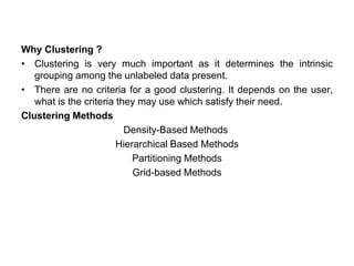
• For ex– The data points in the graph below clustered together can
be classified into one single group.
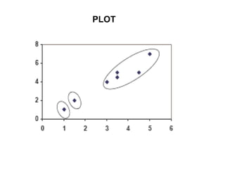
• We can distinguish the clusters, and we can identify that there are 3
clusters in the below picture.
Why Clustering ?
• Clustering is very much important as it determines the intrinsic
grouping among the unlabeled data present.
• There are no criteria for a good clustering. It depends on the user,
what is the criteria they may use which satisfy their need.
Clustering Methods
Density-Based Methods
Hierarchical Based Methods
Partitioning Methods
Grid-based Methods
Applications of Clustering in different fields
1. Marketing : It can be used to characterize & discover customer
segments for marketing purposes.
2. Biology : It can be used for classification among different species of
plants and animals.
3. Libraries : It is used in clustering different books on the basis of
topics and information.
4. Insurance : It is used to acknowledge the customers, their policies
and identifying the frauds.
5. City Planning : It is used to make groups of houses and to study
their values based on their geographical locations and other factors
present.
6. Earthquake studies : By learning the earthquake affected areas we
can determine the dangerous zones.
Common Distance measures
• Distance measure will determine how the similarity of two elements
is calculated and it will influence the shape of the clusters.
They include:
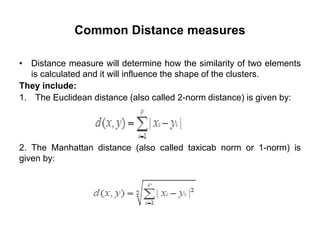
1. The Euclidean distance (also called 2-norm distance) is given by:
2. The Manhattan distance (also called taxicab norm or 1-norm) is
given by:
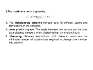
3.The maximum norm is given by:
4. The Mahalanobis distance corrects data for different scales and
correlations in the variables.
5. Inner product space: The angle between two vectors can be used
as a distance measure when clustering high dimensional data
6. Hamming distance (sometimes edit distance) measures the
minimum number of substitutions required to change one member
into another.
K-Means Clustering Algorithm
K-MEANS CLUSTERING
• The k-means algorithm is an algorithm to cluster n objects based
on attributes into k partitions, where k < n.
• It is similar to the expectation-maximization algorithm for mixtures of
Gaussians in that they both attempt to find the centers of natural
clusters in the data.
• It assumes that the object attributes form a vector space.
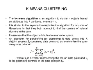
• An algorithm for partitioning (or clustering) N data points into K
disjoint subsets Sj containing data points so as to minimize the sum-
of-squares criterion
- where xn is a vector representing the the nth data point and uj
is the geometric centroid of the data points in Sj.
The algorithm works as follows:
1.First we initialize k points, called means, randomly.
2.We categorize each item to its closest mean and we update the
mean’s coordinates, which are the averages of the items categorized in
that mean so far.
3.We repeat the process for a given number of iterations and at the
end, we have our clusters.
The “points” mentioned above are called means, because they hold the
mean values of the items categorized in it.
-To initialize these means, we have a lot of options. An intuitive
method is to initialize the means at random items in the data set.
- Another method is to initialize the means at random values
between the boundaries of the data set (if for a feature x the items have
values in [0,3], we will initialize the means with values for x at [0,3]).
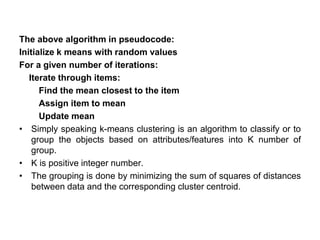
The above algorithm in pseudocode:
Initialize k means with random values
For a given number of iterations:
Iterate through items:
Find the mean closest to the item
Assign item to mean
Update mean
• Simply speaking k-means clustering is an algorithm to classify or to
group the objects based on attributes/features into K number of
group.
• K is positive integer number.
• The grouping is done by minimizing the sum of squares of distances
between data and the corresponding cluster centroid.
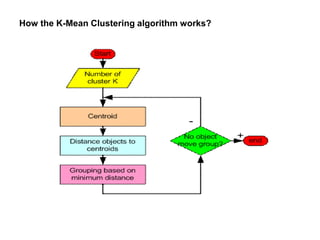
How the K-Mean Clustering algorithm works?
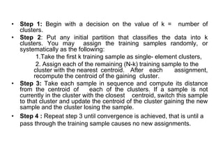
• Step 1: Begin with a decision on the value of k = number of
clusters.
• Step 2: Put any initial partition that classifies the data into k
clusters. You may assign the training samples randomly, or
systematically as the following:
1.Take the first k training sample as single- element clusters,
2. Assign each of the remaining (N-k) training sample to the
cluster with the nearest centroid. After each assignment,
recompute the centroid of the gaining cluster.
• Step 3: Take each sample in sequence and compute its distance
from the centroid of each of the clusters. If a sample is not
currently in the cluster with the closest centroid, switch this sample
to that cluster and update the centroid of the cluster gaining the new
sample and the cluster losing the sample.
• Step 4 : Repeat step 3 until convergence is achieved, that is until a
pass through the training sample causes no new assignments.
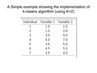
A Simple example showing the implementation of
k-means algorithm (using K=2)
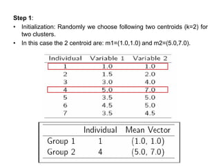
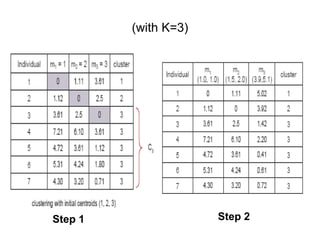
Step 1:
• Initialization: Randomly we choose following two centroids (k=2) for
two clusters.
• In this case the 2 centroid are: m1=(1.0,1.0) and m2=(5.0,7.0).
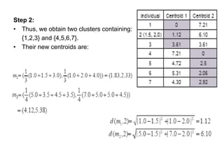
Step 2:
• Thus, we obtain two clusters containing:
{1,2,3} and {4,5,6,7}.
• Their new centroids are:
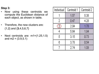
Step 3:
• Now using these centroids we
compute the Euclidean distance of
each object, as shown in table.
• Therefore, the new clusters are:
{1,2} and {3,4,5,6,7}
• Next centroids are: m1=(1.25,1.5)
and m2 = (3.9,5.1)
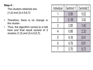
Step 4 :
The clusters obtained are:
{1,2} and {3,4,5,6,7}
• Therefore, there is no change in
the cluster.
• Thus, the algorithm comes to a halt
here and final result consist of 2
clusters {1,2} and {3,4,5,6,7}.
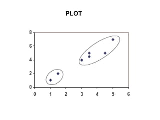
PLOT
(with K=3)
Step 1 Step 2
PLOT
Weaknesses of K-Mean Clustering
1. When the numbers of data are not so many, initial grouping will
determine the cluster significantly.
2. The number of cluster, K, must be determined before hand. Its
disadvantage is that it does not yield the same result with each
run, since the resulting clusters depend on the initial random
assignments.
3. We never know the real cluster, using the same data, because if it
is inputted in a different order it may produce different cluster if the
number of data is few.
4. It is sensitive to initial condition. Different initial condition may
produce different result of cluster. The algorithm may be trapped
in the local optimum.
Applications of K-Mean Clustering
• It is relatively efficient and fast. It computes result at O(tkn), where n
is number of objects or points, k is number of clusters and t is
number of iterations.
• k-means clustering can be applied to machine learning or data
mining
• Used on acoustic data in speech understanding to convert
waveforms into one of k categories (known as Vector Quantization
or Image Segmentation).
• Also used for choosing color palettes on old fashioned graphical
display devices and Image Quantization.
CONCLUSION
• K-means algorithm is useful for undirected knowledge discovery and
is relatively simple. K-means has found wide spread usage in lot of
fields, ranging from unsupervised learning of neural network, Pattern
recognitions, Classification analysis, Artificial intelligence, image
processing, machine vision, and many others.
Vector Quantization
Vector Quantization (VQ)
• Vector quantization (VQ) is a critical step in representing signals in
digital form for computer processing. It has various uses in signal
and image compression and in classification.
• If the signal samples are quantized separately, the operation is
called “scalar quantization.” Consequently, if the samples are
grouped to form vectors, their quantization is called “vector
quantization.”
• The idea of scalar quantization generalizes immediately to vector
quantization (VQ). In this case, we have to perform quantization
over blocks of data, instead of a single scalar value.
• The quantization output is an index value which indicates another
data block (vector) from a finite set of vectors, called the codebook.
The selected vector is usually an approximation of the input data
block.
• Vector quantization (VQ) is a classical quantization technique
from signal processing that allows the modeling of probability
density functions by the distribution of prototype vectors.
• It was originally used for data compression. It works by dividing a
large set of points (vectors) into groups having approximately the
same number of points closest to them.
• Each group is represented by its centroid point, as in k-means and
some other clustering algorithms.
• The density matching property of vector quantization is powerful,
especially for identifying the density of large and high-dimensional
data.
• Since data points are represented by the index of their closest
centroid, commonly occurring data have low error, and rare data
high error.
• This is why VQ is suitable for lossy data compression. It can also
be used for lossy data correction and density estimation.
• Changing the quantization dimension from one (for scalar) to
multiple (for vectors) has many important mathematical and
practical implications.
• VQ produces indices that represent the vector formed by grouping
samples.
• The output index, which is an integer, has little or no physical
relation with the vector it is representing, which is formed by
grouping real or complex valued samples.
• The word “quantization” in VQ comes from the fact that similar
vectors are grouped together and represented by the same index.
• Therefore, many distinct vectors on the multidimensional space are
quantized to a single vector that is represented by the index.
• The number of distinct indices defines the number of quantization
levels. Assigning indices to a number of vectors has practical
applications in compression and classification.
• Vector quantization is based on the competitive learning paradigm,
so it is closely related to the self-organizing map model and
to sparse coding models used in deep learning algorithms such
as autoencoder,
• The important point about VQ is that, we require reproduction
vectors (instead of reproduction levels) that are known by the
encoder and the decoder.
• The encoder takes an input vector, determines the best representing
reproduction vector, and transmits the index of that vector.
• The decoder takes that index, and forms the reproduction vector
because it already knows the reproduction vectors instead of the
original.
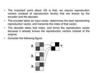
• Consider the following figure:
• The three 2x2 data vectors at the left ( X1 ,X2 , X3) are quantized to
the 2x2 data vector at the right ( Yi ). This means that the encoder
transmits the symbol which represents (Yi) vector when it
encounters the 2x2 vectors at the left as its input.
• Obviously, (Yi) should be a good representation for the left vectors.
The decoder, therefore, reproduces Yi at the places of the original
2x2 vectors at the left.
• The issues of "how good a representation of the right vector is for
the left vectors" is still valid, and the distortion measurements will be
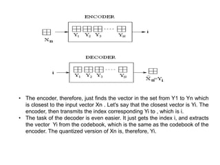
similar to the scalar case. The overall encoder and decoder can be
given as:
• The encoder, therefore, just finds the vector in the set from Y1 to Yn which
is closest to the input vector Xn . Let's say that the closest vector is Yi. The
encoder, then transmits the index corresponding Yi to , which is i.
• The task of the decoder is even easier. It just gets the index i, and extracts
the vector Yi from the codebook, which is the same as the codebook of the
encoder. The quantized version of Xn is, therefore, Yi.
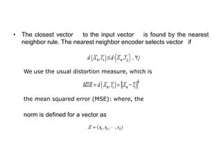
• The closest vector to the input vector is found by the nearest
neighbor rule. The nearest neighbor encoder selects vector if
We use the usual distortion measure, which is
the mean squared error (MSE): where, the
norm is defined for a vector as
Training
The simplest training algorithm for vector quantization is
1.Pick a sample point at random
2.Move the nearest quantization vector centroid towards this sample
point, by a small fraction of the distance
3.Repeat.
Applications
•Vector quantization is used for lossy data compression, lossy data
correction, pattern recognition, density estimation and clustering.
•Lossy data correction, or prediction, is used to recover data missing
from some dimensions.
Principal component analysis
• Principal Component Analysis (PCA) is a dimension-reduction
tool that can be used to reduce a large set of variables to a small set
that still contains most of the information in the large set.
• Principal component analysis (PCA) is a mathematical procedure
that transforms a number of (possibly) correlated variables into a
(smaller) number of uncorrelated variables called principal
components.
• The first principal component accounts for as much of the variability
in the data as possible, and each succeeding component accounts
for as much of the remaining variability as possible.
• Principal components analysis is similar to another multivariate
procedure called Factor Analysis. They are often confused and
many scientists do not understand the difference between the two
methods or what types of analyses they are each best suited.
• Traditionally, principal component analysis is performed on a square
symmetric matrix.
• It can be a SSCP matrix (pure sums of squares and cross products),
Covariance matrix (scaled sums of squares and cross products), or
Correlation matrix (sums of squares and cross products from
standardized data).
• The analysis results for objects of type SSCP and Covariance do not
differ, since these objects only differ in a global scaling factor.
• A correlation matrix is used if the variances of individual variates
differ much, or if the units of measurement of the individual variates
differ.
Objectives of principal component analysis
• PCA reduces attribute space from a larger number of variables to a
smaller number of factors and as such is a "non-dependent" procedure
(that is, it does not assume a dependent variable is specified).
• PCA is a dimensionality reduction or data compression method. The
goal is dimension reduction and there is no guarantee that the
dimensions are interpretable (a fact often not appreciated by (amateur)
statisticians).
•To select a subset of variables from a larger set, based on which
original variables have the highest correlations with the principal
component.
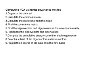
Computing PCA using the covariance method
1.Organize the data set
2.Calculate the empirical mean
3.Calculate the deviations from the mean
4.Find the covariance matrix
5.Find the eigenvectors and eigenvalues of the covariance matrix
6.Rearrange the eigenvectors and eigenvalues
7.Compute the cumulative energy content for each eigenvector
8.Select a subset of the eigenvectors as basis vectors
9.Project the z-scores of the data onto the new basis
Implementing PCA on a 2-D Dataset
Step 1: Normalize the data (get sample code)
• First step is to normalize the data that we have so that PCA works
properly. This is done by subtracting the respective means from the
numbers in the respective column. So if we have two dimensions
X and Y, all X become 𝔁- and all Y become 𝒚-. This produces a
dataset whose mean is zero.
Step 2: Calculate the covariance matrix (get sample code)
• Since the dataset we took is 2-dimensional, this will result in a 2x2
Covariance matrix.
• Please note that Var[X1] = Cov[X1,X1] and Var[X2] = Cov[X2,X2].
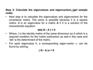
Step 3: Calculate the eigenvalues and eigenvectors (get sample
code)
• Next step is to calculate the eigenvalues and eigenvectors for the
covariance matrix. The same is possible because it is a square
matrix. ƛ is an eigenvalue for a matrix A if it is a solution of the
characteristic equation:
det( ƛI - A ) = 0
• Where, I is the identity matrix of the same dimension as A which is a
required condition for the matrix subtraction as well in this case and
‘det’ is the determinant of the matrix.
• For each eigenvalue ƛ, a corresponding eigen-vector v, can be
found by solving:
( ƛI - A )v = 0
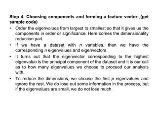
Step 4: Choosing components and forming a feature vector: (get
sample code)
• Order the eigenvalues from largest to smallest so that it gives us the
components in order or significance. Here comes the dimensionality
reduction part.
• If we have a dataset with n variables, then we have the
corresponding n eigenvalues and eigenvectors.
• It turns out that the eigenvector corresponding to the highest
eigenvalue is the principal component of the dataset and it is our call
as to how many eigenvalues we choose to proceed our analysis
with.
• To reduce the dimensions, we choose the first p eigenvalues and
ignore the rest. We do lose out some information in the process, but
if the eigenvalues are small, we do not lose much.
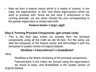
• Next we form a feature vector which is a matrix of vectors, in our
case, the eigenvectors. In fact, only those eigenvectors which we
want to proceed with. Since we just have 2 dimensions in the
running example, we can either choose the one corresponding to
the greater eigenvalue or simply take both.
Feature Vector = (eig1, eig2)
Step 5: Forming Principal Components: (get sample code)
• This is the final step where we actually form the principal
components using all the math we did till here. For the same, we
take the transpose of the feature vector and left-multiply it with the
transpose of scaled version of original dataset.
NewData = FeatureVectorT x ScaledDataT
Here,
NewData is the Matrix consisting of the principal components,
FeatureVector is the matrix we formed using the eigenvectors
we chose to keep, and ScaledData is the scaled version of
original dataset
Limitations
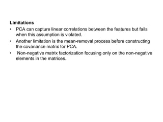
• PCA can capture linear correlations between the features but fails
when this assumption is violated.
• Another limitation is the mean-removal process before constructing
the covariance matrix for PCA.
• Non-negative matrix factorization focusing only on the non-negative
elements in the matrices.
Factor Analysis
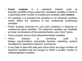
• Factor analysis is a statistical method used to
describe variability among observed, correlated variables in terms of
a potentially lower number of unobserved variables called factors.
• For example, it is possible that variations in six observed variables
mainly reflect the variations in two unobserved (underlying)
variables.
• Factor analysis searches for such joint variations in response to
unobserved latent variables. The observed variables are modelled
as linear combinations of the potential factors, plus "error" terms.
• Factor analysis aims to find independent latent variables.
• Factor analysis is commonly used in
biology, psychometrics, personality theories, marketing, product
management, operations research, and finance.
• It may help to deal with data sets where there are large numbers of
observed variables that are thought to reflect a smaller number of
underlying/latent variables.
• Common factor analysis: Factor model explores a reduced
correlation matrix. That is, communalities (r 2) are inserted on the
diagonal of the correlation matrix, and the extracted factors are
based only on the common variance, with specific and error
variances excluded.
• Common variance: Variance shared with other variables in the
factor analysis.
• Specific or unique variance: Variance of each variable unique to
that variable and not explained or associated with other variables in
the factor analysis.
• Communality: Total amount of variance an original variable shares
with all other variables included in the analysis.
• Eigenvalue: Column sum of squared loadings for a factor; = the
latent root. It conceptually represents that amount of variance
accounted for by a factor.
• Sphericity test: Statistical test for the overall significance of all
correlations within a correlation matrix
• Factor: Linear combination (variate) of the original variables.
Factors also represent the underlying dimensions (constructs) that
summarize or account for the original set of observed variables.
• Factor loadings: Correlation between the original variables and the
factors, and the key to understanding the nature of a particular
factor. Squared factor loadings indicate what percentage of the
variance in an original variable is explained by a factor.
• Factor matrix: Table displaying the factor loadings of all variables
on each factor.
• Factor score: Composite measure created for each observation on
each factor extracted in the factor analysis. The factor weights are
used in conjunction with the original variable values to calculate
each observation's score. The factor scores are standardized to
according to a z-score
• Factor rotation: Process of manipulation or adjusting the factor
axes to achieve a simpler and pragmatically more meaningful factor
solution.
• Oblique factor rotation: Factor rotation computed so that the
extracted factors are correlated. Rather than arbitrarily constraining
the factor rotation to an orthogonal (90 degree angle) solution, the
oblique solution identifies the extent to which each of the factors are
correlated.
• Orthogonal factor rotation: Factor rotation in which the factors are
extracted so that their axes are maintained at 90 degrees. Each
factor is independent of, or orthogonal to, all other factors. The
correlation between teh factors is determined to be zero.
• VARIMAX: One of the most popular orthogonal factor rotation
methods.
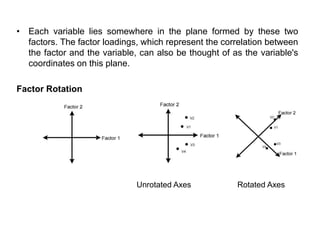
• Each variable lies somewhere in the plane formed by these two
factors. The factor loadings, which represent the correlation between
the factor and the variable, can also be thought of as the variable's
coordinates on this plane.
Factor Rotation
Unrotated Axes Rotated Axes
• In unrotated factor solution the Factor "axes" may not line up very
well with the pattern of variables and the loadings may show no
clear pattern.
• Factor axes can be rotated to more closely correspond to the
variables and therefore become more meaningful. Relative
relationships between variables are preserved.
• The rotation can be either orthogonal or oblique.
Steps in conducting a factor analysis
• There are five basic factor analysis steps:
– Data collection and generation of the correlation matrix
– Partition of variance into common and unique components
(unique may include random error variability)
– Extraction of initial factor solution
– Rotation and interpretation
– Construction of scales or factor scores to use in further analyses
Types of factor analysis
1. Exploratory factor analysis (EFA) is used to identify complex
interrelationships among items and group items that are part of unified
concepts. The researcher makes no a priori assumptions about
relationships among factors.
2. Confirmatory factor analysis (CFA) is a more complex approach
that tests the hypothesis that the items are associated with specific
factors.
• CFA uses structural equation modeling to test a measurement
model whereby loading on the factors allows for evaluation of
relationships between observed variables and unobserved
variables.
• Structural equation modeling approaches can accommodate
measurement error, and are less restrictive than least-squares
estimation.
• Hypothesized models are tested against actual data, and the
analysis would demonstrate loadings of observed variables on the
latent variables (factors), as well as the correlation between the
latent variables.
Advantages
• Reduction of number of variables, by combining two or more
variables into a single factor. For example, performance at running,
ball throwing, batting, jumping and weight lifting could be combined
into a single factor such as general athletic ability.
• Usually, in an item by people matrix, factors are selected by
grouping related items. In the Q factor analysis technique, the matrix
is transposed and factors are created by grouping related people:
For example, liberals, libertarians, conservatives and socialists,
could form separate groups.
Disadvantage
• Factor analysis can be only as good as the data allows. In
psychology, where researchers often have to rely on less valid and
reliable measures such as self-reports, this can be problematic.
Independent Component
Analysis
• Independent Component Analysis (ICA) is a machine learning
technique to separate independent sources from a mixed signal.
• Unlike principal component analysis which focuses on maximizing
the variance of the data points, the independent component analysis
focuses on independence, i.e. independent components.
• Independent component analysis attempts to decompose a
multivariate signal into independent non-Gaussian signals.
• The ICA separation of mixed signals gives very good results is
based on two assumptions and three effects of mixing source
signals. Two assumptions:
1. The source signals are independent of each other.
2. The values in each source signal have non-Gaussian distributions.
• Three effects of mixing source signals:
1.Independence: As per assumption 1, the source signals are
independent; however, their signal mixtures are not. This is because
the signal mixtures share the same source signals.
2. Normality: According to the Central Limit Theorem, the
distribution of a sum of independent random variables with finite
variance tends towards a Gaussian distribution.
Loosely speaking, a sum of two independent random variables usually
has a distribution that is closer to Gaussian than any of the two original
variables. Here we consider the value of each signal as the random
variable.
3.Complexity: The temporal complexity of any signal mixture
is greater than that of its simplest constituent source signal.
• Problem: To extract independent sources’ signals from a mixed
signal composed of the signals from those sources.
• Given: Mixed signal from five different independent sources.
• Aim: To decompose the mixed signal into independent sources:
– Source 1
– Source 2
– Source 3
– Source 4
– Source 5
Solution: Independent Component Analysis (ICA).
Consider Cocktail Party Problem or Blind Source Separation
problem to understand the problem which is solved by independent
component analysis.
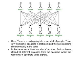
• Here, There is a party going into a room full of people. There
is ‘n’ number of speakers in that room and they are speaking
simultaneously at the party.
• In the same room, there are also ‘n’ number of microphones
placed at different distances from the speakers which are
recording ‘n’ speakers’ voice signals.
• Hence, the number of speakers is equal to the number must of
microphones in the room.
• Now, using these microphones’ recordings, we want to separate all
the ‘n’ speakers’ voice signals in the room given each microphone
recorded the voice signals coming from each speaker of different
intensity due to the difference in distances between them.
• Decomposing the mixed signal of each microphone’s recording into
independent source’s speech signal can be done by using the
machine learning technique, independent component analysis.
[ X1, X2, ….., Xn ] => [ Y1, Y2, ….., Yn ]
- where, X1, X2, …, Xn are the original signals present in the
mixed signal and Y1, Y2, …, Yn are the new features and are
independent components which are independent of each other.
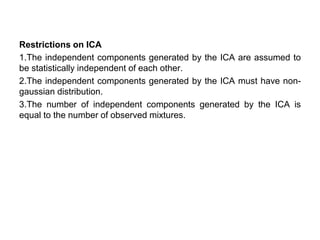
Restrictions on ICA
1.The independent components generated by the ICA are assumed to
be statistically independent of each other.
2.The independent components generated by the ICA must have non-
gaussian distribution.
3.The number of independent components generated by the ICA is
equal to the number of observed mixtures.
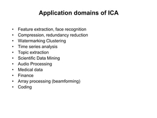
Application domains of ICA
• Feature extraction, face recognition
• Compression, redundancy reduction
• Watermarking Clustering
• Time series analysis
• Topic extraction
• Scientific Data Mining
• Audio Processing
• Medical data
• Finance
• Array processing (beamforming)
• Coding
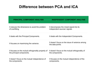
Difference between PCA and ICA
PRINCIPAL COMPONENT ANALYSIS INDEPENDENT COMPONENT ANALYSIS
It reduces the dimensions to avoid the problem
of overfitting.
It decomposes the mixed signal into its
independent sources’ signals.
It deals with the Principal Components. It deals with the Independent Components.
It focuses on maximizing the variance.
It doesn’t focus on the issue of variance among
the data points.
It focuses on the mutual orthogonality property of
the principal components.
It doesn’t focus on the mutual orthogonality of
the components.
It doesn’t focus on the mutual independence of
the components.
It focuses on the mutual independence of the
components.
Locally Linear Embedding
• Locally linear embedding (LLE) seeks a lower-dimensional
projection of the data which preserves distances within local
neighborhoods.
• It can be thought of as a series of local Principal Component
Analyses which are globally compared to find the best non-linear
embedding.
• Locally linear embedding can be performed with function
locally_linear_embedding or its object-oriented counterpart
LocallyLinearEmbedding.
• Locally Linear Embedding (LLE) is a method of Non Linear
Dimensionality reduction.
• Dimensionality reduction helps reduce the complexity of the
machine learning model helping reduce overfitting to an extent.
• Data sets can often be represented in a n-Dimensional feature
space, with each dimension used for a specific feature.
• The LLE algorithm is an unsupervised method for dimensionality
reduction.
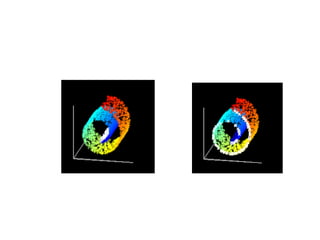
• It tries to reduce these n-Dimensions while trying to preserve the
geometric features of the original non-linear feature structure.
• For example, in the below illustration, we cast the structure of the
swiss roll into a lower dimensional plane, while maintaining its
geometric structure.
• In short, if we have D dimensions for data X1, we try to reduce X1 to
X2 in a feature space with d dimensions.
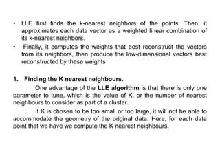
• LLE first finds the k-nearest neighbors of the points. Then, it
approximates each data vector as a weighted linear combination of
its k-nearest neighbors.
• Finally, it computes the weights that best reconstruct the vectors
from its neighbors, then produce the low-dimensional vectors best
reconstructed by these weights
1. Finding the K nearest neighbours.
One advantage of the LLE algorithm is that there is only one
parameter to tune, which is the value of K, or the number of nearest
neighbours to consider as part of a cluster.
If K is chosen to be too small or too large, it will not be able to
accommodate the geometry of the original data. Here, for each data
point that we have we compute the K nearest neighbours.
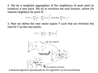
2. We do a weighted aggregation of the neighbours of each point to
construct a new point. We try to minimize the cost function, where j’th
nearest neighbour for point Xi.
3. Now we define the new vector space Y such that we minimize the
cost for Y as the new points.
A detailed algorithm pseudocode for this algorithm can be found below.
Input X: D by N matrix consisting of N data items in D dimensions.
Output Y: d by N matrix consisting of d < D dimensional embedding
coordinates for the input points.
1. Find neighbours in X space [b,c].
for i=1:N
compute the distance from Xi to every other point Xj
find the K smallest distances
assign the corresponding points to be neighbours of Xi
end
2. Solve for reconstruction weights W
for i=1:N
create matrix Z consisting of all neighbours of Xi [d]
subtract Xi from every column of Z
compute the local covariance C=Z'*Z [e]
solve linear system C*w = 1 for w [f]
set Wij=0 if j is not a neighbor of i
set the remaining elements in the ith row of W equal to
w/sum(w);
3. Compute embedding coordinates Y using weights W.
create sparse matrix M = (I-W)'*(I-W)
find bottom d+1 eigenvectors of M
(corresponding to the d+1 smallest eigenvalues)
set the qth ROW of Y to be the q+1 smallest eigenvector
(discard the bottom eigenvector [1,1,1,1...] with
eigenvalue zero)
Advantages of LLE
Better computational time
Consideration of the non-linearity of the structure
Applications
Data visualization
Information retrieval
Image process
Pattern recognition
Isomap
• Isomap is a nonlinear dimensionality reduction method. It is one of
several widely used low-dimensional embedding methods.
• Isomap is used for computing a quasi-isometric, low-dimensional
embedding of a set of high-dimensional data points.
• The algorithm provides a simple method for estimating the intrinsic
geometry of a data manifold based on a rough estimate of each data
point’s neighbors on the manifold.
• Isomap is highly efficient and generally applicable to a broad range
of data sources and dimensionalities.
• Isomap is one representative of isometric mapping methods, and
extends metric multidimensional scaling (MDS) by incorporating the
geodesic distances imposed by a weighted graph.
• Isomap is distinguished by its use of the geodesic distance induced
by a neighborhood graph embedded in the classical scaling.
• Isomap defines the geodesic distance to be the sum of edge weights
along the shortest path between two nodes (computed
using Dijkstra's algorithm, for example).
• The top n eigenvectors of the geodesic distance matrix, represent
the coordinates in the new n-dimensional Euclidean space.
A very high-level description of Isomap algorithm is given below.
Determine the neighbors of each point.
– All points in some fixed radius.
– K nearest neighbors.
Construct a neighborhood graph.
– Each point is connected to other if it is a K nearest neighbor.
– Edge length equal to Euclidean distance.
Compute shortest path between two nodes.
– Dijkstra's algorithm
– Floyd–Warshall algorithm
Compute lower-dimensional embedding.
– Multidimensional scaling
Extensions of ISOMAP
1. LandMark ISOMAP (L-ISOMAP): Landmark-Isomap is a variant of
Isomap which is faster than Isomap. However, the accuracy of the
manifold is compromised by a marginal factor.
In this algorithm, n << N landmark points are used out of the total N
data points and an nxN matrix of the geodesic distance between each
data point to the landmark points is computed.
Landmark-MDS (LMDS) is then applied on the matrix to find a
Euclidean embedding of all the data points.
2. C Isomap : C-Isomap involves magnifying the regions of high
density and shrink the regions of low density of data points in the
manifold. Edge weights that are maximized in Multi-Dimensional
Scaling(MDS) are modified, with everything else remaining unaffected.
3. Parallel Transport Unfolding : Replaces the Dijkstra path-based
geodesic distance estimates with parallel transport based
approximations instead, improving robustness to irregularity and voids
in the sampling
Possible issues
• The connectivity of each data point in the neighborhood graph is
defined as its nearest k Euclidean neighbors in the high-dimensional
space.
• This step is vulnerable to "short-circuit errors" if k is too large with
respect to the manifold structure or if noise in the data moves the
points slightly off the manifold.
• Even a single short-circuit error can alter many entries in the
geodesic distance matrix, which in turn can lead to a drastically
different (and incorrect) low-dimensional embedding.
• Conversely, if k is too small, the neighborhood graph may become
too sparse to approximate geodesic paths accurately. But
improvements have been made to this algorithm to make it work
better for sparse and noisy data sets.[5]
Least Square Optimization
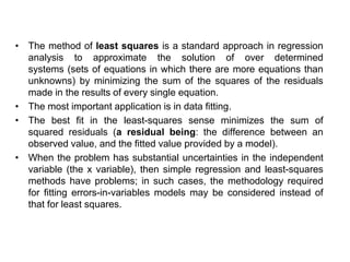
• The method of least squares is a standard approach in regression
analysis to approximate the solution of over determined
systems (sets of equations in which there are more equations than
unknowns) by minimizing the sum of the squares of the residuals
made in the results of every single equation.
• The most important application is in data fitting.
• The best fit in the least-squares sense minimizes the sum of
squared residuals (a residual being: the difference between an
observed value, and the fitted value provided by a model).
• When the problem has substantial uncertainties in the independent
variable (the x variable), then simple regression and least-squares
methods have problems; in such cases, the methodology required
for fitting errors-in-variables models may be considered instead of
that for least squares.
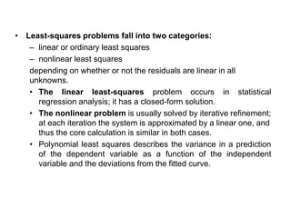
• Least-squares problems fall into two categories:
– linear or ordinary least squares
– nonlinear least squares
depending on whether or not the residuals are linear in all
unknowns.
• The linear least-squares problem occurs in statistical
regression analysis; it has a closed-form solution.
• The nonlinear problem is usually solved by iterative refinement;
at each iteration the system is approximated by a linear one, and
thus the core calculation is similar in both cases.
• Polynomial least squares describes the variance in a prediction
of the dependent variable as a function of the independent
variable and the deviations from the fitted curve.
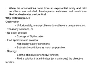
• When the observations come from an exponential family and mild
conditions are satisfied, least-squares estimates and maximum-
likelihood estimates are identical.
Why Optimization..?
Observation
– Unfortunately, many problems do not have a unique solution.
• Too many solutions, or
• No exact solution
– Concept of Optimization
• Find approximated solution
– Not exactly satisfy conditions,
– But satisfy conditions as much as possible.
• Strategy
– Set the objective (or energy) function
– Find a solution that minimizes (or maximizes) the objective
function.
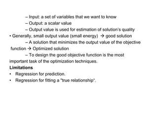
– Input: a set of variables that we want to know
– Output: a scalar value
– Output value is used for estimation of solution’s quality
• Generally, small output value (small energy) → good solution
– A solution that minimizes the output value of the objective
function → Optimized solution
– To design the good objective function is the most
important task of the optimization techniques.
Limitations
• Regression for prediction.
• Regression for fitting a "true relationship“.
Simulated annealing
• SA is a global optimization technique.
• SA distinguishes between different local optima.
• SA is a memory less algorithm, the algorithm does not use any
information gathered during the search
• SA is motivated by an analogy to annealing in solids.
• Simulated Annealing – an iterative improvement algorithm.
Background: Annealing
• Simulated annealing is so named because of its analogy to the
process of physical annealing with solids,.
• A crystalline solid is heated and then allowed to cool very slowly
until it achieves its most regular possible crystal lattice configuration
(i.e., its minimum lattice energy state), and thus is free of crystal
defects.
• If the cooling schedule is sufficiently slow, the final configuration
results in a solid with such superior structural integrity.
• Simulated annealing establishes the connection between this type of
thermodynamic behavior and the search for global minima for a
discrete optimization problem.
• Solid is heated to melting point
- High-energy, high-entropy state
- Removes defects/irregularities
• Temp is very slowly reduced
- Recrystallization occurs (regular structure)
- New internal state of diffused atoms
- Fast cooling induces fragile structure
Example
• Annealing in metals
• Heat the solid state metal to a high temperature
• Cool it down very slowly according to a specific schedule.
• If the heating temperature is sufficiently high to ensure random state
and the cooling process is slow enough to ensure thermal
equilibrium, then the atoms will place themselves in a pattern that
corresponds to the global energy minimum of a perfect crystal.
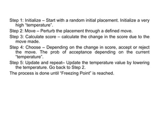
Step 1: Initialize – Start with a random initial placement. Initialize a very
high “temperature”.
Step 2: Move – Perturb the placement through a defined move.
Step 3: Calculate score – calculate the change in the score due to the
move made.
Step 4: Choose – Depending on the change in score, accept or reject
the move. The prob of acceptance depending on the current
“temperature”.
Step 5: Update and repeat– Update the temperature value by lowering
the temperature. Go back to Step 2.
The process is done until “Freezing Point” is reached.
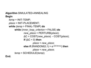
Algorithm SIMULATED-ANNEALING
Begin
temp = INIT-TEMP;
place = INIT-PLACEMENT;
while (temp > FINAL-TEMP) do
while (inner_loop_criterion = FALSE) do
new_place = PERTURB(place);
ΔC = COST(new_place) - COST(place);
if (ΔC < 0) then
place = new_place;
else if (RANDOM(0,1) > e-(ΔC/temp)) then
place = new_place;
temp = SCHEDULE(temp);
End.
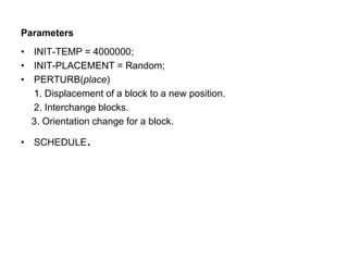
Parameters
• INIT-TEMP = 4000000;
• INIT-PLACEMENT = Random;
• PERTURB(place)
1. Displacement of a block to a new position.
2. Interchange blocks.
3. Orientation change for a block.
• SCHEDULE.
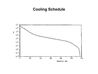
Cooling Schedule
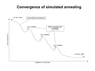
Convergence of simulated annealing
HILL CLIMBING
HILL CLIMBING
HILL CLIMBING
COSTFUNCTION,C
NUMBER OF ITERATIONS
AT INIT_TEMP
AT FINAL_TEMP
Move accepted with
probability
= e-(^C/temp)
Unconditional Acceptance
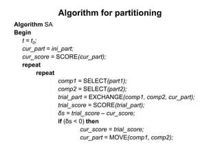
Algorithm for partitioning
Algorithm SA
Begin
t = t0;
cur_part = ini_part;
cur_score = SCORE(cur_part);
repeat
repeat
comp1 = SELECT(part1);
comp2 = SELECT(part2);
trial_part = EXCHANGE(comp1, comp2, cur_part);
trial_score = SCORE(trial_part);
δs = trial_score – cur_score;
if (δs < 0) then
cur_score = trial_score;
cur_part = MOVE(comp1, comp2);
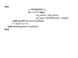
else
r = RANDOM(0,1);
if (r < e-(δs/t)) then
cur_score = trial_score;
cur_part = MOVE(comp1, comp2);
until (equilibrium at t is reached)
t = αt (0 < α < 1)
until (freezing point is reached)
End.
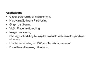
Applications
• Circuit partitioning and placement.
• Hardware/Software Partitioning
• Graph partitioning
• VLSI: Placement, routing.
• Image processing
• Strategy scheduling for capital products with complex product
structure.
• Umpire scheduling in US Open Tennis tournament!
• Event-based learning situations.
Advantages
• can deal with arbitrary systems and cost functions
• statistically guarantees finding an optimal solution
• It is relatively easy to code, even for complex problems.
• generally gives a ``good'' solution This makes annealing an
attractive option for optimization problems where heuristic
(specialized or problem specific) methods are not available.
Disadvantages
• Repeatedly annealing with a 1/log k schedule is very slow,
especially if the cost function is expensive to compute.
• Heuristic methods, which are problem-specific or take advantage of
extra information about the system, will often be better than general
methods, although SA is often comparable to heuristics.
• The method cannot tell whether it has found an optimal solution.
Some other complimentary method (e.g. branch and bound) is
required to do this

CSA 3702 machine learning module 3

  • 1.
    CSA 3702 –MACHINE LEARNING PREPARED BY, NANDHINI S (SRMIST, RAMAPURAM CAMPUS), BHARATHI RAJA N, MENNAKSHI COLLEGE OF ENGINEERING.
  • 2.
  • 3.
  • 4.
    What is clustering? •Clustering: the process of grouping a set of objects into classes of similar objects – Documents within a cluster should be similar. – Documents from different clusters should be dissimilar. • Clustering is the task of dividing the data points into a number of groups such that data points in the same groups are more similar to other data points in the same group and dissimilar to the data points in other groups. • It is basically a collection of objects on the basis of similarity and dissimilarity between them.
  • 5.
    • For ex–The data points in the graph below clustered together can be classified into one single group. • We can distinguish the clusters, and we can identify that there are 3 clusters in the below picture.
  • 6.
    Why Clustering ? •Clustering is very much important as it determines the intrinsic grouping among the unlabeled data present. • There are no criteria for a good clustering. It depends on the user, what is the criteria they may use which satisfy their need. Clustering Methods Density-Based Methods Hierarchical Based Methods Partitioning Methods Grid-based Methods
  • 7.
    Applications of Clusteringin different fields 1. Marketing : It can be used to characterize & discover customer segments for marketing purposes. 2. Biology : It can be used for classification among different species of plants and animals. 3. Libraries : It is used in clustering different books on the basis of topics and information. 4. Insurance : It is used to acknowledge the customers, their policies and identifying the frauds. 5. City Planning : It is used to make groups of houses and to study their values based on their geographical locations and other factors present. 6. Earthquake studies : By learning the earthquake affected areas we can determine the dangerous zones.
  • 8.
    Common Distance measures •Distance measure will determine how the similarity of two elements is calculated and it will influence the shape of the clusters. They include: 1. The Euclidean distance (also called 2-norm distance) is given by: 2. The Manhattan distance (also called taxicab norm or 1-norm) is given by:
  • 9.
    3.The maximum normis given by: 4. The Mahalanobis distance corrects data for different scales and correlations in the variables. 5. Inner product space: The angle between two vectors can be used as a distance measure when clustering high dimensional data 6. Hamming distance (sometimes edit distance) measures the minimum number of substitutions required to change one member into another.
  • 10.
  • 11.
    K-MEANS CLUSTERING • Thek-means algorithm is an algorithm to cluster n objects based on attributes into k partitions, where k < n. • It is similar to the expectation-maximization algorithm for mixtures of Gaussians in that they both attempt to find the centers of natural clusters in the data. • It assumes that the object attributes form a vector space. • An algorithm for partitioning (or clustering) N data points into K disjoint subsets Sj containing data points so as to minimize the sum- of-squares criterion - where xn is a vector representing the the nth data point and uj is the geometric centroid of the data points in Sj.
  • 12.
    The algorithm worksas follows: 1.First we initialize k points, called means, randomly. 2.We categorize each item to its closest mean and we update the mean’s coordinates, which are the averages of the items categorized in that mean so far. 3.We repeat the process for a given number of iterations and at the end, we have our clusters. The “points” mentioned above are called means, because they hold the mean values of the items categorized in it. -To initialize these means, we have a lot of options. An intuitive method is to initialize the means at random items in the data set. - Another method is to initialize the means at random values between the boundaries of the data set (if for a feature x the items have values in [0,3], we will initialize the means with values for x at [0,3]).
  • 13.
    The above algorithmin pseudocode: Initialize k means with random values For a given number of iterations: Iterate through items: Find the mean closest to the item Assign item to mean Update mean • Simply speaking k-means clustering is an algorithm to classify or to group the objects based on attributes/features into K number of group. • K is positive integer number. • The grouping is done by minimizing the sum of squares of distances between data and the corresponding cluster centroid.
  • 14.
    How the K-MeanClustering algorithm works?
  • 15.
    • Step 1:Begin with a decision on the value of k = number of clusters. • Step 2: Put any initial partition that classifies the data into k clusters. You may assign the training samples randomly, or systematically as the following: 1.Take the first k training sample as single- element clusters, 2. Assign each of the remaining (N-k) training sample to the cluster with the nearest centroid. After each assignment, recompute the centroid of the gaining cluster. • Step 3: Take each sample in sequence and compute its distance from the centroid of each of the clusters. If a sample is not currently in the cluster with the closest centroid, switch this sample to that cluster and update the centroid of the cluster gaining the new sample and the cluster losing the sample. • Step 4 : Repeat step 3 until convergence is achieved, that is until a pass through the training sample causes no new assignments.
  • 16.
    A Simple exampleshowing the implementation of k-means algorithm (using K=2)
  • 17.
    Step 1: • Initialization:Randomly we choose following two centroids (k=2) for two clusters. • In this case the 2 centroid are: m1=(1.0,1.0) and m2=(5.0,7.0).
  • 18.
    Step 2: • Thus,we obtain two clusters containing: {1,2,3} and {4,5,6,7}. • Their new centroids are:
  • 19.
    Step 3: • Nowusing these centroids we compute the Euclidean distance of each object, as shown in table. • Therefore, the new clusters are: {1,2} and {3,4,5,6,7} • Next centroids are: m1=(1.25,1.5) and m2 = (3.9,5.1)
  • 20.
    Step 4 : Theclusters obtained are: {1,2} and {3,4,5,6,7} • Therefore, there is no change in the cluster. • Thus, the algorithm comes to a halt here and final result consist of 2 clusters {1,2} and {3,4,5,6,7}.
  • 21.
  • 22.
  • 23.
  • 24.
    Weaknesses of K-MeanClustering 1. When the numbers of data are not so many, initial grouping will determine the cluster significantly. 2. The number of cluster, K, must be determined before hand. Its disadvantage is that it does not yield the same result with each run, since the resulting clusters depend on the initial random assignments. 3. We never know the real cluster, using the same data, because if it is inputted in a different order it may produce different cluster if the number of data is few. 4. It is sensitive to initial condition. Different initial condition may produce different result of cluster. The algorithm may be trapped in the local optimum.
  • 25.
    Applications of K-MeanClustering • It is relatively efficient and fast. It computes result at O(tkn), where n is number of objects or points, k is number of clusters and t is number of iterations. • k-means clustering can be applied to machine learning or data mining • Used on acoustic data in speech understanding to convert waveforms into one of k categories (known as Vector Quantization or Image Segmentation). • Also used for choosing color palettes on old fashioned graphical display devices and Image Quantization.
  • 26.
    CONCLUSION • K-means algorithmis useful for undirected knowledge discovery and is relatively simple. K-means has found wide spread usage in lot of fields, ranging from unsupervised learning of neural network, Pattern recognitions, Classification analysis, Artificial intelligence, image processing, machine vision, and many others.
  • 27.
  • 28.
    Vector Quantization (VQ) •Vector quantization (VQ) is a critical step in representing signals in digital form for computer processing. It has various uses in signal and image compression and in classification. • If the signal samples are quantized separately, the operation is called “scalar quantization.” Consequently, if the samples are grouped to form vectors, their quantization is called “vector quantization.” • The idea of scalar quantization generalizes immediately to vector quantization (VQ). In this case, we have to perform quantization over blocks of data, instead of a single scalar value. • The quantization output is an index value which indicates another data block (vector) from a finite set of vectors, called the codebook. The selected vector is usually an approximation of the input data block.
  • 29.
    • Vector quantization(VQ) is a classical quantization technique from signal processing that allows the modeling of probability density functions by the distribution of prototype vectors. • It was originally used for data compression. It works by dividing a large set of points (vectors) into groups having approximately the same number of points closest to them. • Each group is represented by its centroid point, as in k-means and some other clustering algorithms. • The density matching property of vector quantization is powerful, especially for identifying the density of large and high-dimensional data. • Since data points are represented by the index of their closest centroid, commonly occurring data have low error, and rare data high error. • This is why VQ is suitable for lossy data compression. It can also be used for lossy data correction and density estimation. • Changing the quantization dimension from one (for scalar) to multiple (for vectors) has many important mathematical and practical implications.
  • 30.
    • VQ producesindices that represent the vector formed by grouping samples. • The output index, which is an integer, has little or no physical relation with the vector it is representing, which is formed by grouping real or complex valued samples. • The word “quantization” in VQ comes from the fact that similar vectors are grouped together and represented by the same index. • Therefore, many distinct vectors on the multidimensional space are quantized to a single vector that is represented by the index. • The number of distinct indices defines the number of quantization levels. Assigning indices to a number of vectors has practical applications in compression and classification. • Vector quantization is based on the competitive learning paradigm, so it is closely related to the self-organizing map model and to sparse coding models used in deep learning algorithms such as autoencoder,
  • 31.
    • The importantpoint about VQ is that, we require reproduction vectors (instead of reproduction levels) that are known by the encoder and the decoder. • The encoder takes an input vector, determines the best representing reproduction vector, and transmits the index of that vector. • The decoder takes that index, and forms the reproduction vector because it already knows the reproduction vectors instead of the original. • Consider the following figure:
  • 32.
    • The three2x2 data vectors at the left ( X1 ,X2 , X3) are quantized to the 2x2 data vector at the right ( Yi ). This means that the encoder transmits the symbol which represents (Yi) vector when it encounters the 2x2 vectors at the left as its input. • Obviously, (Yi) should be a good representation for the left vectors. The decoder, therefore, reproduces Yi at the places of the original 2x2 vectors at the left. • The issues of "how good a representation of the right vector is for the left vectors" is still valid, and the distortion measurements will be similar to the scalar case. The overall encoder and decoder can be given as:
  • 33.
    • The encoder,therefore, just finds the vector in the set from Y1 to Yn which is closest to the input vector Xn . Let's say that the closest vector is Yi. The encoder, then transmits the index corresponding Yi to , which is i. • The task of the decoder is even easier. It just gets the index i, and extracts the vector Yi from the codebook, which is the same as the codebook of the encoder. The quantized version of Xn is, therefore, Yi.
  • 34.
    • The closestvector to the input vector is found by the nearest neighbor rule. The nearest neighbor encoder selects vector if We use the usual distortion measure, which is the mean squared error (MSE): where, the norm is defined for a vector as
  • 35.
    Training The simplest trainingalgorithm for vector quantization is 1.Pick a sample point at random 2.Move the nearest quantization vector centroid towards this sample point, by a small fraction of the distance 3.Repeat. Applications •Vector quantization is used for lossy data compression, lossy data correction, pattern recognition, density estimation and clustering. •Lossy data correction, or prediction, is used to recover data missing from some dimensions.
  • 36.
  • 37.
    • Principal ComponentAnalysis (PCA) is a dimension-reduction tool that can be used to reduce a large set of variables to a small set that still contains most of the information in the large set. • Principal component analysis (PCA) is a mathematical procedure that transforms a number of (possibly) correlated variables into a (smaller) number of uncorrelated variables called principal components. • The first principal component accounts for as much of the variability in the data as possible, and each succeeding component accounts for as much of the remaining variability as possible. • Principal components analysis is similar to another multivariate procedure called Factor Analysis. They are often confused and many scientists do not understand the difference between the two methods or what types of analyses they are each best suited.
  • 38.
    • Traditionally, principalcomponent analysis is performed on a square symmetric matrix. • It can be a SSCP matrix (pure sums of squares and cross products), Covariance matrix (scaled sums of squares and cross products), or Correlation matrix (sums of squares and cross products from standardized data). • The analysis results for objects of type SSCP and Covariance do not differ, since these objects only differ in a global scaling factor. • A correlation matrix is used if the variances of individual variates differ much, or if the units of measurement of the individual variates differ.
  • 39.
    Objectives of principalcomponent analysis • PCA reduces attribute space from a larger number of variables to a smaller number of factors and as such is a "non-dependent" procedure (that is, it does not assume a dependent variable is specified). • PCA is a dimensionality reduction or data compression method. The goal is dimension reduction and there is no guarantee that the dimensions are interpretable (a fact often not appreciated by (amateur) statisticians). •To select a subset of variables from a larger set, based on which original variables have the highest correlations with the principal component.
  • 40.
    Computing PCA usingthe covariance method 1.Organize the data set 2.Calculate the empirical mean 3.Calculate the deviations from the mean 4.Find the covariance matrix 5.Find the eigenvectors and eigenvalues of the covariance matrix 6.Rearrange the eigenvectors and eigenvalues 7.Compute the cumulative energy content for each eigenvector 8.Select a subset of the eigenvectors as basis vectors 9.Project the z-scores of the data onto the new basis
  • 41.
    Implementing PCA ona 2-D Dataset Step 1: Normalize the data (get sample code) • First step is to normalize the data that we have so that PCA works properly. This is done by subtracting the respective means from the numbers in the respective column. So if we have two dimensions X and Y, all X become 𝔁- and all Y become 𝒚-. This produces a dataset whose mean is zero. Step 2: Calculate the covariance matrix (get sample code) • Since the dataset we took is 2-dimensional, this will result in a 2x2 Covariance matrix. • Please note that Var[X1] = Cov[X1,X1] and Var[X2] = Cov[X2,X2].
  • 42.
    Step 3: Calculatethe eigenvalues and eigenvectors (get sample code) • Next step is to calculate the eigenvalues and eigenvectors for the covariance matrix. The same is possible because it is a square matrix. ƛ is an eigenvalue for a matrix A if it is a solution of the characteristic equation: det( ƛI - A ) = 0 • Where, I is the identity matrix of the same dimension as A which is a required condition for the matrix subtraction as well in this case and ‘det’ is the determinant of the matrix. • For each eigenvalue ƛ, a corresponding eigen-vector v, can be found by solving: ( ƛI - A )v = 0
  • 43.
    Step 4: Choosingcomponents and forming a feature vector: (get sample code) • Order the eigenvalues from largest to smallest so that it gives us the components in order or significance. Here comes the dimensionality reduction part. • If we have a dataset with n variables, then we have the corresponding n eigenvalues and eigenvectors. • It turns out that the eigenvector corresponding to the highest eigenvalue is the principal component of the dataset and it is our call as to how many eigenvalues we choose to proceed our analysis with. • To reduce the dimensions, we choose the first p eigenvalues and ignore the rest. We do lose out some information in the process, but if the eigenvalues are small, we do not lose much.
  • 44.
    • Next weform a feature vector which is a matrix of vectors, in our case, the eigenvectors. In fact, only those eigenvectors which we want to proceed with. Since we just have 2 dimensions in the running example, we can either choose the one corresponding to the greater eigenvalue or simply take both. Feature Vector = (eig1, eig2) Step 5: Forming Principal Components: (get sample code) • This is the final step where we actually form the principal components using all the math we did till here. For the same, we take the transpose of the feature vector and left-multiply it with the transpose of scaled version of original dataset. NewData = FeatureVectorT x ScaledDataT Here, NewData is the Matrix consisting of the principal components, FeatureVector is the matrix we formed using the eigenvectors we chose to keep, and ScaledData is the scaled version of original dataset
  • 45.
    Limitations • PCA cancapture linear correlations between the features but fails when this assumption is violated. • Another limitation is the mean-removal process before constructing the covariance matrix for PCA. • Non-negative matrix factorization focusing only on the non-negative elements in the matrices.
  • 46.
  • 47.
    • Factor analysisis a statistical method used to describe variability among observed, correlated variables in terms of a potentially lower number of unobserved variables called factors. • For example, it is possible that variations in six observed variables mainly reflect the variations in two unobserved (underlying) variables. • Factor analysis searches for such joint variations in response to unobserved latent variables. The observed variables are modelled as linear combinations of the potential factors, plus "error" terms. • Factor analysis aims to find independent latent variables. • Factor analysis is commonly used in biology, psychometrics, personality theories, marketing, product management, operations research, and finance. • It may help to deal with data sets where there are large numbers of observed variables that are thought to reflect a smaller number of underlying/latent variables.
  • 48.
    • Common factoranalysis: Factor model explores a reduced correlation matrix. That is, communalities (r 2) are inserted on the diagonal of the correlation matrix, and the extracted factors are based only on the common variance, with specific and error variances excluded. • Common variance: Variance shared with other variables in the factor analysis. • Specific or unique variance: Variance of each variable unique to that variable and not explained or associated with other variables in the factor analysis. • Communality: Total amount of variance an original variable shares with all other variables included in the analysis. • Eigenvalue: Column sum of squared loadings for a factor; = the latent root. It conceptually represents that amount of variance accounted for by a factor.
  • 49.
    • Sphericity test:Statistical test for the overall significance of all correlations within a correlation matrix • Factor: Linear combination (variate) of the original variables. Factors also represent the underlying dimensions (constructs) that summarize or account for the original set of observed variables. • Factor loadings: Correlation between the original variables and the factors, and the key to understanding the nature of a particular factor. Squared factor loadings indicate what percentage of the variance in an original variable is explained by a factor. • Factor matrix: Table displaying the factor loadings of all variables on each factor. • Factor score: Composite measure created for each observation on each factor extracted in the factor analysis. The factor weights are used in conjunction with the original variable values to calculate each observation's score. The factor scores are standardized to according to a z-score
  • 50.
    • Factor rotation:Process of manipulation or adjusting the factor axes to achieve a simpler and pragmatically more meaningful factor solution. • Oblique factor rotation: Factor rotation computed so that the extracted factors are correlated. Rather than arbitrarily constraining the factor rotation to an orthogonal (90 degree angle) solution, the oblique solution identifies the extent to which each of the factors are correlated. • Orthogonal factor rotation: Factor rotation in which the factors are extracted so that their axes are maintained at 90 degrees. Each factor is independent of, or orthogonal to, all other factors. The correlation between teh factors is determined to be zero. • VARIMAX: One of the most popular orthogonal factor rotation methods.
  • 51.
    • Each variablelies somewhere in the plane formed by these two factors. The factor loadings, which represent the correlation between the factor and the variable, can also be thought of as the variable's coordinates on this plane. Factor Rotation Unrotated Axes Rotated Axes
  • 52.
    • In unrotatedfactor solution the Factor "axes" may not line up very well with the pattern of variables and the loadings may show no clear pattern. • Factor axes can be rotated to more closely correspond to the variables and therefore become more meaningful. Relative relationships between variables are preserved. • The rotation can be either orthogonal or oblique.
  • 53.
    Steps in conductinga factor analysis • There are five basic factor analysis steps: – Data collection and generation of the correlation matrix – Partition of variance into common and unique components (unique may include random error variability) – Extraction of initial factor solution – Rotation and interpretation – Construction of scales or factor scores to use in further analyses
  • 54.
    Types of factoranalysis 1. Exploratory factor analysis (EFA) is used to identify complex interrelationships among items and group items that are part of unified concepts. The researcher makes no a priori assumptions about relationships among factors. 2. Confirmatory factor analysis (CFA) is a more complex approach that tests the hypothesis that the items are associated with specific factors. • CFA uses structural equation modeling to test a measurement model whereby loading on the factors allows for evaluation of relationships between observed variables and unobserved variables. • Structural equation modeling approaches can accommodate measurement error, and are less restrictive than least-squares estimation. • Hypothesized models are tested against actual data, and the analysis would demonstrate loadings of observed variables on the latent variables (factors), as well as the correlation between the latent variables.
  • 55.
    Advantages • Reduction ofnumber of variables, by combining two or more variables into a single factor. For example, performance at running, ball throwing, batting, jumping and weight lifting could be combined into a single factor such as general athletic ability. • Usually, in an item by people matrix, factors are selected by grouping related items. In the Q factor analysis technique, the matrix is transposed and factors are created by grouping related people: For example, liberals, libertarians, conservatives and socialists, could form separate groups. Disadvantage • Factor analysis can be only as good as the data allows. In psychology, where researchers often have to rely on less valid and reliable measures such as self-reports, this can be problematic.
  • 56.
  • 57.
    • Independent ComponentAnalysis (ICA) is a machine learning technique to separate independent sources from a mixed signal. • Unlike principal component analysis which focuses on maximizing the variance of the data points, the independent component analysis focuses on independence, i.e. independent components. • Independent component analysis attempts to decompose a multivariate signal into independent non-Gaussian signals. • The ICA separation of mixed signals gives very good results is based on two assumptions and three effects of mixing source signals. Two assumptions: 1. The source signals are independent of each other. 2. The values in each source signal have non-Gaussian distributions.
  • 58.
    • Three effectsof mixing source signals: 1.Independence: As per assumption 1, the source signals are independent; however, their signal mixtures are not. This is because the signal mixtures share the same source signals. 2. Normality: According to the Central Limit Theorem, the distribution of a sum of independent random variables with finite variance tends towards a Gaussian distribution. Loosely speaking, a sum of two independent random variables usually has a distribution that is closer to Gaussian than any of the two original variables. Here we consider the value of each signal as the random variable. 3.Complexity: The temporal complexity of any signal mixture is greater than that of its simplest constituent source signal.
  • 59.
    • Problem: Toextract independent sources’ signals from a mixed signal composed of the signals from those sources. • Given: Mixed signal from five different independent sources. • Aim: To decompose the mixed signal into independent sources: – Source 1 – Source 2 – Source 3 – Source 4 – Source 5 Solution: Independent Component Analysis (ICA). Consider Cocktail Party Problem or Blind Source Separation problem to understand the problem which is solved by independent component analysis.
  • 60.
    • Here, Thereis a party going into a room full of people. There is ‘n’ number of speakers in that room and they are speaking simultaneously at the party. • In the same room, there are also ‘n’ number of microphones placed at different distances from the speakers which are recording ‘n’ speakers’ voice signals.
  • 61.
    • Hence, thenumber of speakers is equal to the number must of microphones in the room. • Now, using these microphones’ recordings, we want to separate all the ‘n’ speakers’ voice signals in the room given each microphone recorded the voice signals coming from each speaker of different intensity due to the difference in distances between them. • Decomposing the mixed signal of each microphone’s recording into independent source’s speech signal can be done by using the machine learning technique, independent component analysis. [ X1, X2, ….., Xn ] => [ Y1, Y2, ….., Yn ] - where, X1, X2, …, Xn are the original signals present in the mixed signal and Y1, Y2, …, Yn are the new features and are independent components which are independent of each other.
  • 62.
    Restrictions on ICA 1.Theindependent components generated by the ICA are assumed to be statistically independent of each other. 2.The independent components generated by the ICA must have non- gaussian distribution. 3.The number of independent components generated by the ICA is equal to the number of observed mixtures.
  • 63.
    Application domains ofICA • Feature extraction, face recognition • Compression, redundancy reduction • Watermarking Clustering • Time series analysis • Topic extraction • Scientific Data Mining • Audio Processing • Medical data • Finance • Array processing (beamforming) • Coding
  • 64.
    Difference between PCAand ICA PRINCIPAL COMPONENT ANALYSIS INDEPENDENT COMPONENT ANALYSIS It reduces the dimensions to avoid the problem of overfitting. It decomposes the mixed signal into its independent sources’ signals. It deals with the Principal Components. It deals with the Independent Components. It focuses on maximizing the variance. It doesn’t focus on the issue of variance among the data points. It focuses on the mutual orthogonality property of the principal components. It doesn’t focus on the mutual orthogonality of the components. It doesn’t focus on the mutual independence of the components. It focuses on the mutual independence of the components.
  • 65.
  • 66.
    • Locally linearembedding (LLE) seeks a lower-dimensional projection of the data which preserves distances within local neighborhoods. • It can be thought of as a series of local Principal Component Analyses which are globally compared to find the best non-linear embedding. • Locally linear embedding can be performed with function locally_linear_embedding or its object-oriented counterpart LocallyLinearEmbedding. • Locally Linear Embedding (LLE) is a method of Non Linear Dimensionality reduction. • Dimensionality reduction helps reduce the complexity of the machine learning model helping reduce overfitting to an extent.
  • 67.
    • Data setscan often be represented in a n-Dimensional feature space, with each dimension used for a specific feature. • The LLE algorithm is an unsupervised method for dimensionality reduction. • It tries to reduce these n-Dimensions while trying to preserve the geometric features of the original non-linear feature structure. • For example, in the below illustration, we cast the structure of the swiss roll into a lower dimensional plane, while maintaining its geometric structure. • In short, if we have D dimensions for data X1, we try to reduce X1 to X2 in a feature space with d dimensions.
  • 69.
    • LLE firstfinds the k-nearest neighbors of the points. Then, it approximates each data vector as a weighted linear combination of its k-nearest neighbors. • Finally, it computes the weights that best reconstruct the vectors from its neighbors, then produce the low-dimensional vectors best reconstructed by these weights 1. Finding the K nearest neighbours. One advantage of the LLE algorithm is that there is only one parameter to tune, which is the value of K, or the number of nearest neighbours to consider as part of a cluster. If K is chosen to be too small or too large, it will not be able to accommodate the geometry of the original data. Here, for each data point that we have we compute the K nearest neighbours.
  • 70.
    2. We doa weighted aggregation of the neighbours of each point to construct a new point. We try to minimize the cost function, where j’th nearest neighbour for point Xi. 3. Now we define the new vector space Y such that we minimize the cost for Y as the new points. A detailed algorithm pseudocode for this algorithm can be found below.
  • 71.
    Input X: Dby N matrix consisting of N data items in D dimensions. Output Y: d by N matrix consisting of d < D dimensional embedding coordinates for the input points. 1. Find neighbours in X space [b,c]. for i=1:N compute the distance from Xi to every other point Xj find the K smallest distances assign the corresponding points to be neighbours of Xi end 2. Solve for reconstruction weights W for i=1:N create matrix Z consisting of all neighbours of Xi [d] subtract Xi from every column of Z compute the local covariance C=Z'*Z [e] solve linear system C*w = 1 for w [f] set Wij=0 if j is not a neighbor of i set the remaining elements in the ith row of W equal to w/sum(w);
  • 72.
    3. Compute embeddingcoordinates Y using weights W. create sparse matrix M = (I-W)'*(I-W) find bottom d+1 eigenvectors of M (corresponding to the d+1 smallest eigenvalues) set the qth ROW of Y to be the q+1 smallest eigenvector (discard the bottom eigenvector [1,1,1,1...] with eigenvalue zero) Advantages of LLE Better computational time Consideration of the non-linearity of the structure Applications Data visualization Information retrieval Image process Pattern recognition
  • 73.
  • 74.
    • Isomap isa nonlinear dimensionality reduction method. It is one of several widely used low-dimensional embedding methods. • Isomap is used for computing a quasi-isometric, low-dimensional embedding of a set of high-dimensional data points. • The algorithm provides a simple method for estimating the intrinsic geometry of a data manifold based on a rough estimate of each data point’s neighbors on the manifold. • Isomap is highly efficient and generally applicable to a broad range of data sources and dimensionalities. • Isomap is one representative of isometric mapping methods, and extends metric multidimensional scaling (MDS) by incorporating the geodesic distances imposed by a weighted graph.
  • 75.
    • Isomap isdistinguished by its use of the geodesic distance induced by a neighborhood graph embedded in the classical scaling. • Isomap defines the geodesic distance to be the sum of edge weights along the shortest path between two nodes (computed using Dijkstra's algorithm, for example). • The top n eigenvectors of the geodesic distance matrix, represent the coordinates in the new n-dimensional Euclidean space.
  • 76.
    A very high-leveldescription of Isomap algorithm is given below. Determine the neighbors of each point. – All points in some fixed radius. – K nearest neighbors. Construct a neighborhood graph. – Each point is connected to other if it is a K nearest neighbor. – Edge length equal to Euclidean distance. Compute shortest path between two nodes. – Dijkstra's algorithm – Floyd–Warshall algorithm Compute lower-dimensional embedding. – Multidimensional scaling
  • 77.
    Extensions of ISOMAP 1.LandMark ISOMAP (L-ISOMAP): Landmark-Isomap is a variant of Isomap which is faster than Isomap. However, the accuracy of the manifold is compromised by a marginal factor. In this algorithm, n << N landmark points are used out of the total N data points and an nxN matrix of the geodesic distance between each data point to the landmark points is computed. Landmark-MDS (LMDS) is then applied on the matrix to find a Euclidean embedding of all the data points. 2. C Isomap : C-Isomap involves magnifying the regions of high density and shrink the regions of low density of data points in the manifold. Edge weights that are maximized in Multi-Dimensional Scaling(MDS) are modified, with everything else remaining unaffected. 3. Parallel Transport Unfolding : Replaces the Dijkstra path-based geodesic distance estimates with parallel transport based approximations instead, improving robustness to irregularity and voids in the sampling
  • 78.
    Possible issues • Theconnectivity of each data point in the neighborhood graph is defined as its nearest k Euclidean neighbors in the high-dimensional space. • This step is vulnerable to "short-circuit errors" if k is too large with respect to the manifold structure or if noise in the data moves the points slightly off the manifold. • Even a single short-circuit error can alter many entries in the geodesic distance matrix, which in turn can lead to a drastically different (and incorrect) low-dimensional embedding. • Conversely, if k is too small, the neighborhood graph may become too sparse to approximate geodesic paths accurately. But improvements have been made to this algorithm to make it work better for sparse and noisy data sets.[5]
  • 79.
  • 80.
    • The methodof least squares is a standard approach in regression analysis to approximate the solution of over determined systems (sets of equations in which there are more equations than unknowns) by minimizing the sum of the squares of the residuals made in the results of every single equation. • The most important application is in data fitting. • The best fit in the least-squares sense minimizes the sum of squared residuals (a residual being: the difference between an observed value, and the fitted value provided by a model). • When the problem has substantial uncertainties in the independent variable (the x variable), then simple regression and least-squares methods have problems; in such cases, the methodology required for fitting errors-in-variables models may be considered instead of that for least squares.
  • 81.
    • Least-squares problemsfall into two categories: – linear or ordinary least squares – nonlinear least squares depending on whether or not the residuals are linear in all unknowns. • The linear least-squares problem occurs in statistical regression analysis; it has a closed-form solution. • The nonlinear problem is usually solved by iterative refinement; at each iteration the system is approximated by a linear one, and thus the core calculation is similar in both cases. • Polynomial least squares describes the variance in a prediction of the dependent variable as a function of the independent variable and the deviations from the fitted curve.
  • 82.
    • When theobservations come from an exponential family and mild conditions are satisfied, least-squares estimates and maximum- likelihood estimates are identical. Why Optimization..? Observation – Unfortunately, many problems do not have a unique solution. • Too many solutions, or • No exact solution – Concept of Optimization • Find approximated solution – Not exactly satisfy conditions, – But satisfy conditions as much as possible. • Strategy – Set the objective (or energy) function – Find a solution that minimizes (or maximizes) the objective function.
  • 83.
    – Input: aset of variables that we want to know – Output: a scalar value – Output value is used for estimation of solution’s quality • Generally, small output value (small energy) → good solution – A solution that minimizes the output value of the objective function → Optimized solution – To design the good objective function is the most important task of the optimization techniques. Limitations • Regression for prediction. • Regression for fitting a "true relationship“.
  • 84.
  • 85.
    • SA isa global optimization technique. • SA distinguishes between different local optima. • SA is a memory less algorithm, the algorithm does not use any information gathered during the search • SA is motivated by an analogy to annealing in solids. • Simulated Annealing – an iterative improvement algorithm. Background: Annealing • Simulated annealing is so named because of its analogy to the process of physical annealing with solids,. • A crystalline solid is heated and then allowed to cool very slowly until it achieves its most regular possible crystal lattice configuration (i.e., its minimum lattice energy state), and thus is free of crystal defects.
  • 86.
    • If thecooling schedule is sufficiently slow, the final configuration results in a solid with such superior structural integrity. • Simulated annealing establishes the connection between this type of thermodynamic behavior and the search for global minima for a discrete optimization problem. • Solid is heated to melting point - High-energy, high-entropy state - Removes defects/irregularities • Temp is very slowly reduced - Recrystallization occurs (regular structure) - New internal state of diffused atoms - Fast cooling induces fragile structure
  • 87.
    Example • Annealing inmetals • Heat the solid state metal to a high temperature • Cool it down very slowly according to a specific schedule. • If the heating temperature is sufficiently high to ensure random state and the cooling process is slow enough to ensure thermal equilibrium, then the atoms will place themselves in a pattern that corresponds to the global energy minimum of a perfect crystal.
  • 88.
    Step 1: Initialize– Start with a random initial placement. Initialize a very high “temperature”. Step 2: Move – Perturb the placement through a defined move. Step 3: Calculate score – calculate the change in the score due to the move made. Step 4: Choose – Depending on the change in score, accept or reject the move. The prob of acceptance depending on the current “temperature”. Step 5: Update and repeat– Update the temperature value by lowering the temperature. Go back to Step 2. The process is done until “Freezing Point” is reached.
  • 89.
    Algorithm SIMULATED-ANNEALING Begin temp =INIT-TEMP; place = INIT-PLACEMENT; while (temp > FINAL-TEMP) do while (inner_loop_criterion = FALSE) do new_place = PERTURB(place); ΔC = COST(new_place) - COST(place); if (ΔC < 0) then place = new_place; else if (RANDOM(0,1) > e-(ΔC/temp)) then place = new_place; temp = SCHEDULE(temp); End.
  • 90.
    Parameters • INIT-TEMP =4000000; • INIT-PLACEMENT = Random; • PERTURB(place) 1. Displacement of a block to a new position. 2. Interchange blocks. 3. Orientation change for a block. • SCHEDULE.
  • 91.
  • 92.
    Convergence of simulatedannealing HILL CLIMBING HILL CLIMBING HILL CLIMBING COSTFUNCTION,C NUMBER OF ITERATIONS AT INIT_TEMP AT FINAL_TEMP Move accepted with probability = e-(^C/temp) Unconditional Acceptance
  • 93.
    Algorithm for partitioning AlgorithmSA Begin t = t0; cur_part = ini_part; cur_score = SCORE(cur_part); repeat repeat comp1 = SELECT(part1); comp2 = SELECT(part2); trial_part = EXCHANGE(comp1, comp2, cur_part); trial_score = SCORE(trial_part); δs = trial_score – cur_score; if (δs < 0) then cur_score = trial_score; cur_part = MOVE(comp1, comp2);
  • 94.
    else r = RANDOM(0,1); if(r < e-(δs/t)) then cur_score = trial_score; cur_part = MOVE(comp1, comp2); until (equilibrium at t is reached) t = αt (0 < α < 1) until (freezing point is reached) End.
  • 95.
    Applications • Circuit partitioningand placement. • Hardware/Software Partitioning • Graph partitioning • VLSI: Placement, routing. • Image processing • Strategy scheduling for capital products with complex product structure. • Umpire scheduling in US Open Tennis tournament! • Event-based learning situations.
  • 96.
    Advantages • can dealwith arbitrary systems and cost functions • statistically guarantees finding an optimal solution • It is relatively easy to code, even for complex problems. • generally gives a ``good'' solution This makes annealing an attractive option for optimization problems where heuristic (specialized or problem specific) methods are not available. Disadvantages • Repeatedly annealing with a 1/log k schedule is very slow, especially if the cost function is expensive to compute. • Heuristic methods, which are problem-specific or take advantage of extra information about the system, will often be better than general methods, although SA is often comparable to heuristics. • The method cannot tell whether it has found an optimal solution. Some other complimentary method (e.g. branch and bound) is required to do this