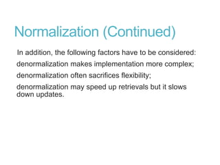
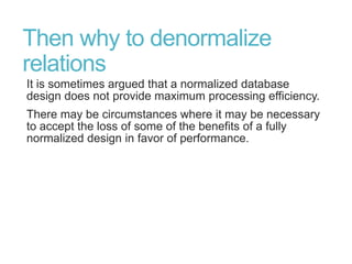
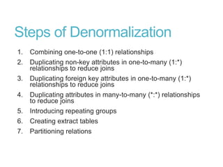
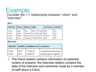
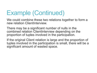
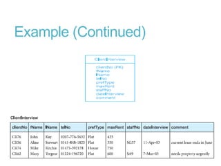
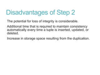
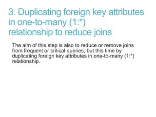
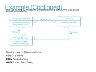
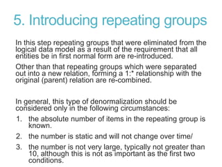
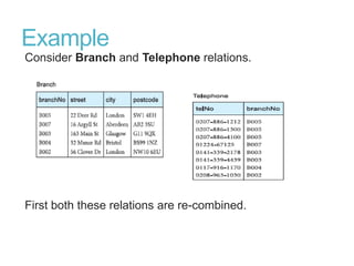
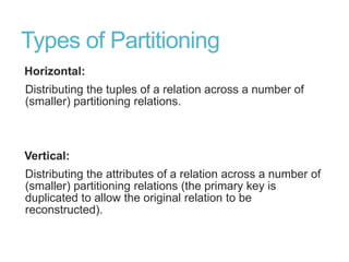
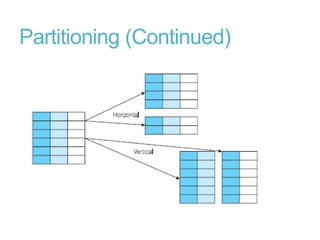
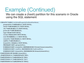
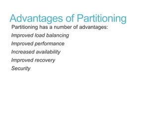
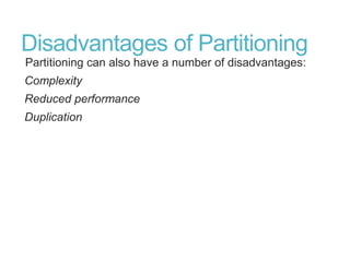
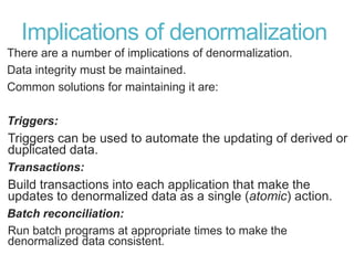
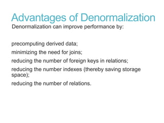
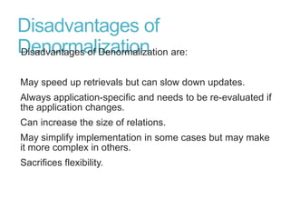
This document discusses denormalization, which refers to modifying a relational schema to be less normalized by combining relations or duplicating attributes. It describes 7 common denormalization techniques: 1) combining one-to-one relations, 2) duplicating attributes in one-to-many relations, 3) duplicating foreign keys, 4) duplicating attributes in many-to-many relations, 5) introducing repeating groups, 6) creating extract tables, and 7) partitioning relations. While denormalization can improve performance, it can also increase complexity, reduce flexibility, and slow down updates. Data integrity must be maintained when denormalizing.

1. Database
Systems
Presentation

2. Topic: Denormalization
Group Members:
Sohail Haider
Abdul Wahab
Mehmood Akhter

3. What is Denormalization
Denormalization refers to a refinement to the relational
schema such that the degree of normalization for a
modified relation is less than the degree of at least one of
the original relations.
Denormalization can also be referred to a process in
which we combine two relations into one new relation,
and the new relation is still normalized but contains more
nulls than the original relations.

4. Normalization
Normalization is a logical database design that is
structurally consistent and has minimal redundancy.
Normalization forces us to understand completely each
attribute that has to be represented in the database. This
may be the most important factor that contributes to the
overall success of the system.

5. Normalization (Continued)
In addition, the following factors have to be considered:
denormalization makes implementation more complex;
denormalization often sacrifices flexibility;
denormalization may speed up retrievals but it slows
down updates.

6. Then why to denormalize
relations
It is sometimes argued that a normalized database
design does not provide maximum processing efficiency.
There may be circumstances where it may be necessary
to accept the loss of some of the benefits of a fully
normalized design in favor of performance.

7. Steps of Denormalization
1. Combining one-to-one (1:1) relationships
2. Duplicating non-key attributes in one-to-many (1:*)
relationships to reduce joins
3. Duplicating foreign key attributes in one-to-many (1:*)
relationships to reduce joins
4. Duplicating attributes in many-to-many (*:*) relationships
to reduce joins
5. Introducing repeating groups
6. Creating extract tables
7. Partitioning relations

9. 1. Combining one-to-one (1:1)
relationships
Re-examine one-to-one (1:1) relationships to determine
the effects of combining the relations into a single
relation.
Combination should only be considered for relations that
are frequently referenced together and infrequently
referenced separately.

10. Example
Consider the 1:1 relationship between “client” and
“interview”.
• The Client relation contains information on potential
renters of property; the Interview relation contains the
date of the interview and comments made by a member
of staff about a Client.

11. Example (Continued)
We could combine these two relations together to form a
new relation ClientInterview.
There may be a significant number of nulls in the
combined relation ClientInterview depending on the
proportion of tuples involved in the participation.
If the original Client relation is large and the proportion of
tuples involved in the participation is small, there will be a
significant amount of wasted space.

12. Example (Continued)

13. 2. Duplicating non-key attributes in
one-to-many (1:*) relationships to
reduce joins
In this step we aim to reduce or remove joins from
frequent or critical queries by duplicating non-key
attributes in 1:* relationships.

14. Example
Consider the relations PropertyForRent and PrivateOwner.

15. Example (Continued)
Whenever the PropertyForRent relation is accessed, it is
very common for the owner‟s name to be accessed at the
same time.
We need to write the following query everytime to access
this:

16. Example (Continued)
By duplicating the lName attribute in the PropertyForRent
relation, PrivateOwner relation can be removed from the
query.

17. Disadvantages of Step 2
The potential for loss of integrity is considerable.
Additional time that is required to maintain consistency
automatically every time a tuple is inserted, updated, or
deleted.
Increase in storage space resulting from the duplication.

18. 3. Duplicating foreign key attributes
in one-to-many (1:*)
relationship to reduce joins
The aim of this step is also to reduce or remove joins
from frequent or critical queries, but this time by
duplicating foreign key attributes in one-to-many (1:*)
relationship.

19. Example
Again consider the relations PropertyForRent and
PrivateOwner.

20. Example (Continued)
In order to list all the private property owners at a branch,
following query will be used:
SELECT o.lName
FROM PropertyForRent p, PrivateOwner o
WHERE p.ownerNo = o.ownerNo AND branchNo =
„B003‟;
The need for this join can be removed by duplicating the
foreign key branchNo in the PrivateOwner relation.

21. Example (Continued)This can be done by introducing a direct relationship between the Branch and
PrivateOwner relations.
Thus the query could be simplified to:
SELECT o.lName
FROM PrivateOwner o
WHERE branchNo = „B003‟;

22. Example (Continued)

23. Before:
SELECT o.lName
FROM PropertyForRent p, PrivateOwner o
WHERE p.ownerNo = o.ownerNo AND branchNo = „B003‟;
After:
SELECT o.lName
FROM PrivateOwner o
WHERE branchNo = „B003‟;

24. 4. Duplicating attributes in many-
to-many (*:*) relationships to
reduce joins
In some circumstances, it may be possible to reduce the
number of relations to be joined by duplicating attributes
from one of the original entities in the intermediate
relation.

25. Example
Consider the relations Client, PropertyForRent and
Viewing.

26. Example (Continued)
Suppose that sales staff need to contact clients who have
still to make a comment on the properties they have
viewed. They need only the street attribute of the property
when talking to the clients. The query for this will be:

27. Example (Continued)
Duplicating the street attribute in the intermediate Viewing
relation can remove the PropertyForRent relation from
the query, giving the query:
SELECT c.*, v.street, v.viewDate
FROM Client c, Viewing v
WHERE c.clientNo = v.clientNo AND comment IS NULL;

28. 5. Introducing repeating groups
In this step repeating groups that were eliminated from the
logical data model as a result of the requirement that all
entities be in first normal form are re-introduced.
Other than that repeating groups which were separated
out into a new relation, forming a 1:* relationship with the
original (parent) relation are re-combined.
In general, this type of denormalization should be
considered only in the following circumstances:
1. the absolute number of items in the repeating group is
known.
2. the number is static and will not change over time/
3. the number is not very large, typically not greater than
10, although this is not as important as the first two
conditions.

29. Example
Consider Branch and Telephone relations.
First both these relations are re-combined.

30. Example (Continued)
then telephone details in the original Branch relation, with
one attribute for each telephone as follows:

31. 6. Creating extract tables
In this step a single, highly denormalized extract table
based on the relations required by the reports.
It allow the users to access the extract table directly
instead of the base relations.

32. Why to create extract tables
This may be for situations where reports have to be run at
peak times during the day.
The most common technique for producing extract tables
is to create and populate the tables in an overnight batch
run when the system is lightly loaded.

33. 7. Partitioning relations
Decomposing relations into a number of smaller and more
manageable pieces called partitions.
This is an alternative approach that addresses the key
problem with supporting very large relations (and indexes)
rather than combining relations together.
There are two main types of partitioning:
1. Horizontal partitioning
2. Vertical partitioning.

34. Types of Partitioning
Horizontal:
Distributing the tuples of a relation across a number of
(smaller) partitioning relations.
Vertical:
Distributing the attributes of a relation across a number of
(smaller) partitioning relations (the primary key is
duplicated to allow the original relation to be
reconstructed).

35. Partitioning (Continued)

36. Other types of Partitioning
Range:
In this type each partition is defined by a range of values
for one or more attributes.
List
In this type each partition is defined by a list of values for
an attribute.
Range–hash and List–hash:
In this type each partition is defined by a range or a list of
values and then each partition is further subdivided based
on a hash function

37. Example (Horizontal
Partitioning)
Suppose DreamHome maintains an
ArchivedPropertyForRent relation with several hundreds
of thousands of tuples that are held indefinitely for analysis
purposes.
Searching for a particular tuple at a branch could be quite
time consuming.
We could reduce this time by horizontally partitioning the
relation, with one partition for each branch.

38. Example (Continued)
We can create a (hash) partition for this scenario in Oracle
using the SQL statement

39. Advantages of Partitioning
Partitioning has a number of advantages:
Improved load balancing
Improved performance
Increased availability
Improved recovery
Security

40. Disadvantages of Partitioning
Partitioning can also have a number of disadvantages:
Complexity
Reduced performance
Duplication

41. Implications of denormalization
There are a number of implications of denormalization.
Data integrity must be maintained.
Common solutions for maintaining it are:
Triggers:
Triggers can be used to automate the updating of derived or
duplicated data.
Transactions:
Build transactions into each application that make the
updates to denormalized data as a single (atomic) action.
Batch reconciliation:
Run batch programs at appropriate times to make the
denormalized data consistent.

42. Advantages of Denormalization
Denormalization can improve performance by:
precomputing derived data;
minimizing the need for joins;
reducing the number of foreign keys in relations;
reducing the number indexes (thereby saving storage
space);
reducing the number of relations.

43. Disadvantages of
DenormalizationDisadvantages of Denormalization are:
May speed up retrievals but can slow down updates.
Always application-specific and needs to be re-evaluated if
the application changes.
Can increase the size of relations.
May simplify implementation in some cases but may make
it more complex in others.
Sacrifices flexibility.

44. Questions?

45. Thank you