Download to read offline


![Process Capability Analysis for Non-Normal Distributions Example
Box-Cox transformation seems confirm the log data transformation.
> boxcox(ceramic$Concentricity ~ 1)
−2 −1 0 1 2
−1100−1050−1000−950−900
λ
log−Likelihood
95%
Process Capability Analysis 65 / 68
Process Capability Analysis for Non-Normal Distributions Example
Capability analysis can be performed directly on log-normal data.
> usl = 30
> par(mfrow = c(1, 1))
> hist(ceramic$Concentricity, main = "Concentricity", col = "gray")
> abline(v = usl, col = "red", lwd = 2)
> concentricity.distpars = fitdistr(ceramic$Concentricity, "log-normal")$estimate
> meanlog = concentricity.distpars[1]
> sdlog = concentricity.distpars[2]
> cpk = usl/qlnorm(0.99865, meanlog, sdlog)
> ppm = (1 - plnorm(30, meanlog, sdlog) * 10^6
Concentricity
ceramic$Concentricity
Frequency
0 10 20 30 40
0204060
Process Capability Analysis 66 / 68](https://image.slidesharecdn.com/cp-cpkparadistribucionesnonormales-201023170156/75/Cp-cpk-para-distribuciones-no-normales-33-2048.jpg)
![Process Capability Analysis for Non-Normal Distributions Example
Results obtained directly on log-normal data can be compared with
transformed data.
> cpk # original data
[1] 0.4886823
> pcr.Concentricity$cpk # transformed data
[1] 0.6149203
> ppm # original data
[1] 32200.77
> pcr.Concentricity$ppt * 10^6 # transformed data
[1] 32536.18
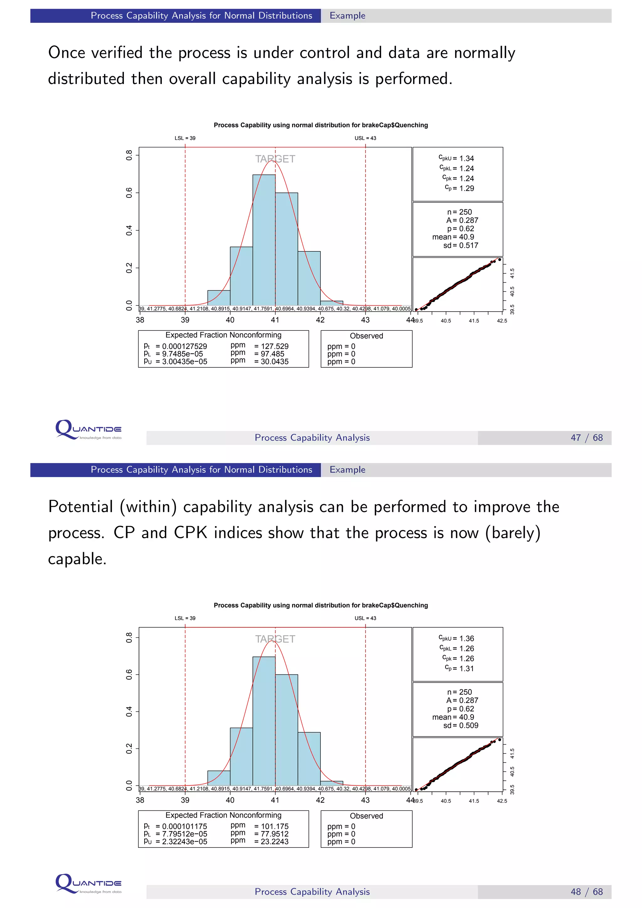
Regardless the adopted methodology to estimate indices, the process is far
from been capable.
Process Capability Analysis 67 / 68
References
References
Montgomery, D.C. (1997). Introduction to Statistical Quality Control. Wiley.
Roth, T. (2010). Working with the qualityTools Package.
http://www.r-qualitytools.org
Roth, T. (2011). Process Capability Statistics for Non-Normal Distributions in R.
http://www.r-qualitytools.org/useR2011/ProcessCapabilityInR.pdf
Kapadia, M. Measuring Your Process Capability.
http://www.symphonytech.com/articles/processcapability.htm
Scrucca, L. (2004). qcc: an R package for Quality Control Charting and Statistical
Process Control. R News 4/1, 11-17.
Roth, T. (2011). qualityTools: Statistics in Quality Science. R package version
1.50.
Process Capability Analysis 68 / 68](https://image.slidesharecdn.com/cp-cpkparadistribucionesnonormales-201023170156/75/Cp-cpk-para-distribuciones-no-normales-34-2048.jpg)

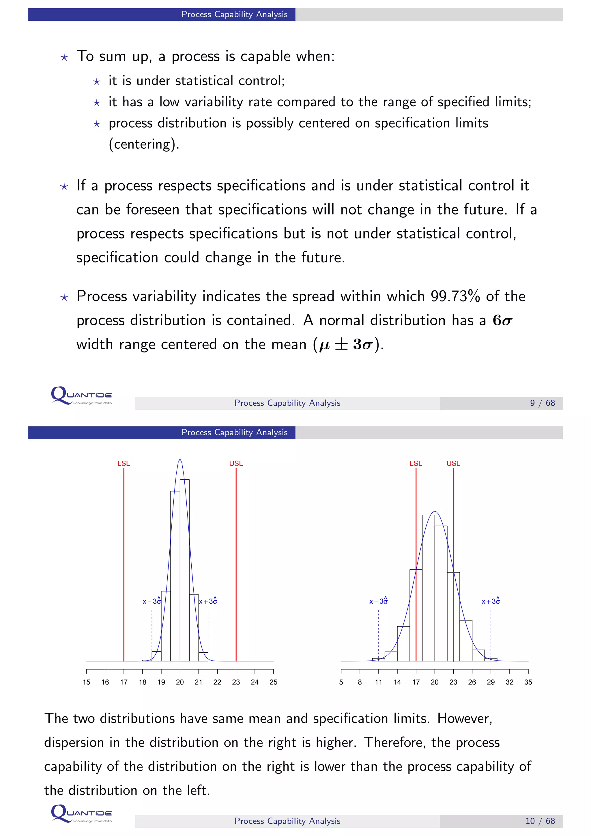
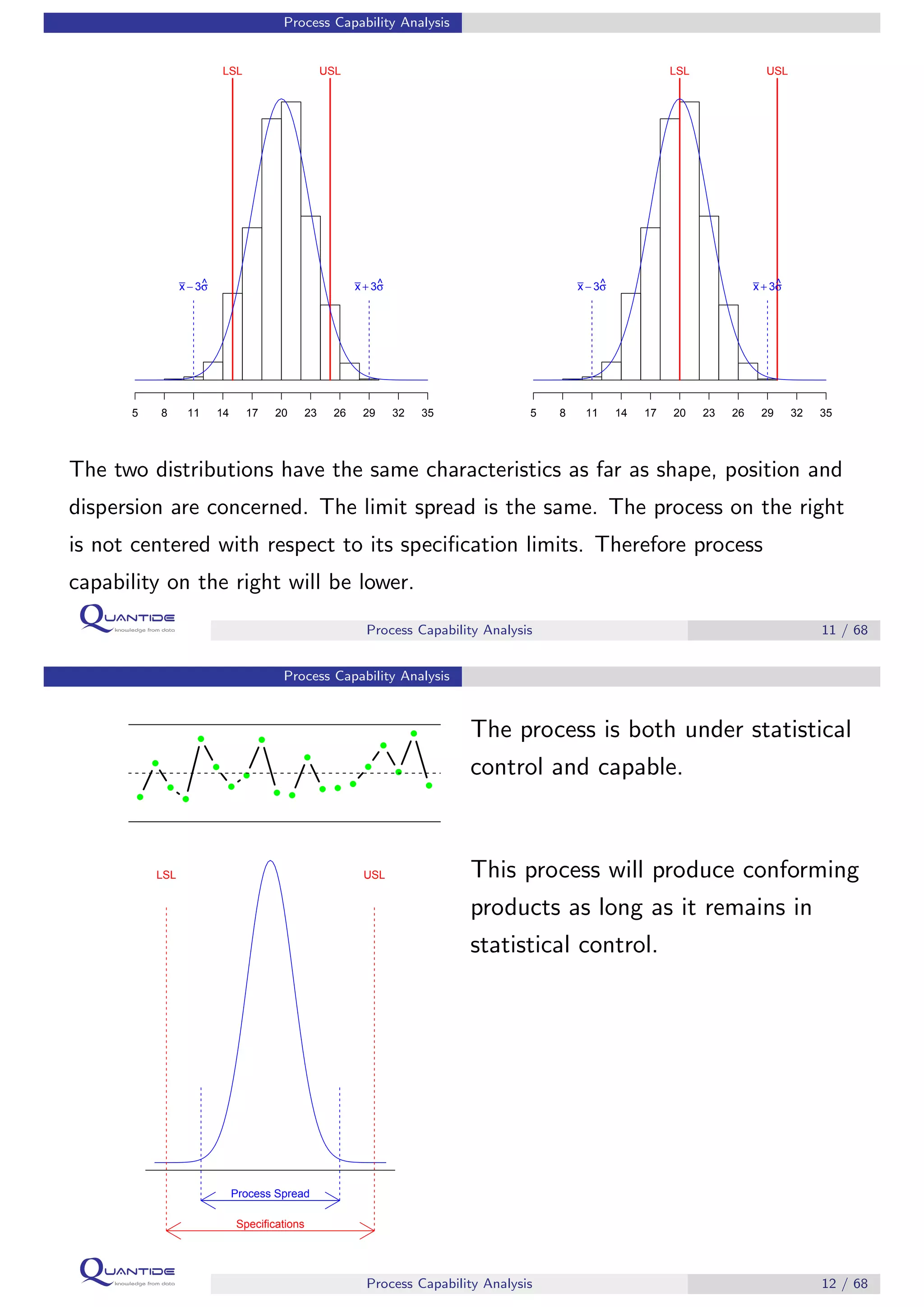
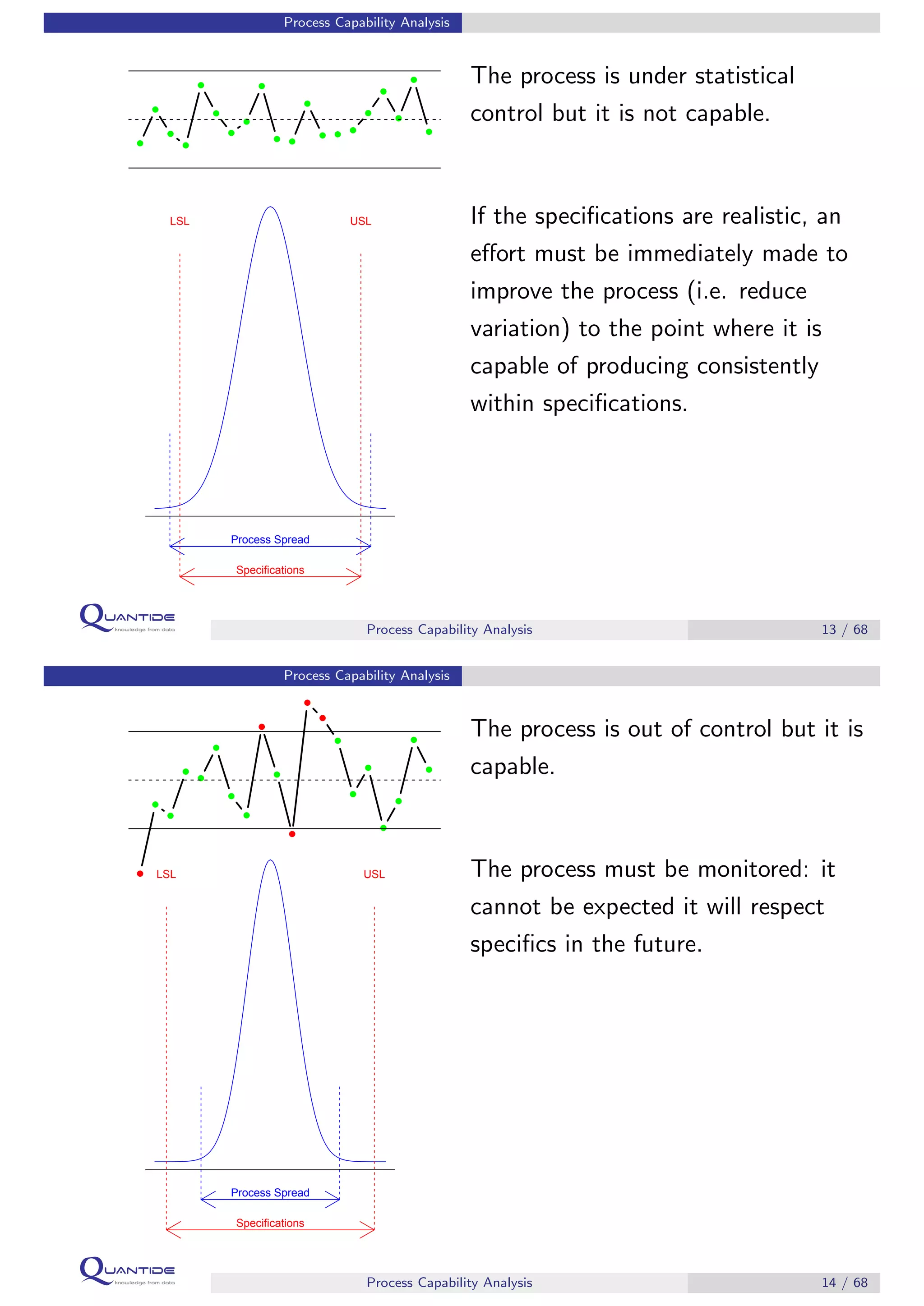
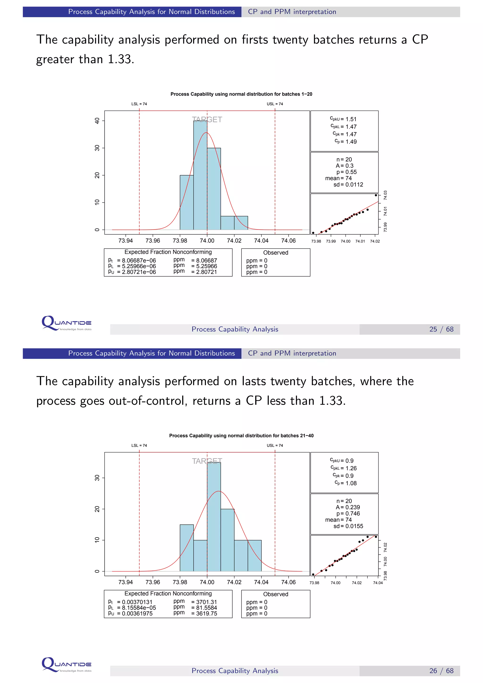
The document discusses process capability analysis, which involves analyzing process data to determine if a process is capable of meeting specifications. It covers calculating capability indices like CP and PPM for normal distributions to quantify a process's capability. CP greater than 1.33 indicates a capable process that should produce less than 64 defective parts per million. The document provides examples of control charts and a sample capability analysis calculation.


![Spc training[1]](https://cdn.slidesharecdn.com/ss_thumbnails/spctraining1-191004152539-thumbnail.jpg?width=640&height=640&fit=bounds)


![Process Capability[1]](https://cdn.slidesharecdn.com/ss_thumbnails/processcapability1-1226090261326164-9-thumbnail.jpg?width=640&height=640&fit=bounds)


