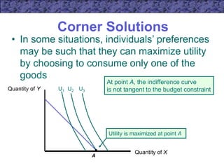
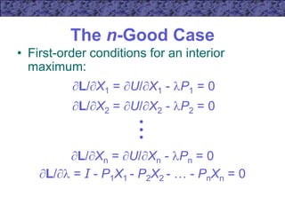
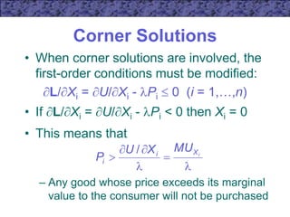
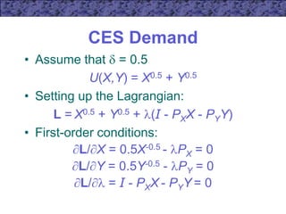
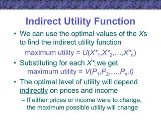
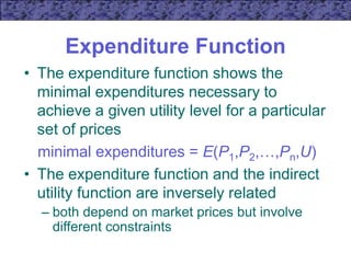
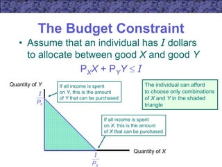
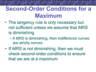
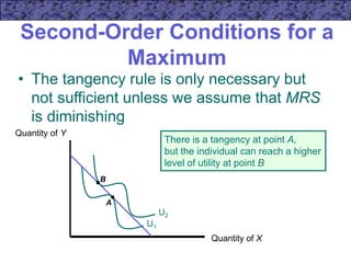
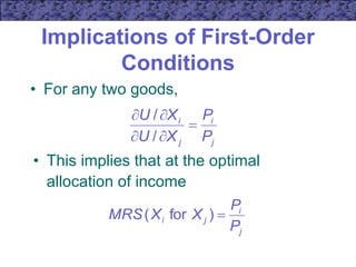
1) The document discusses the economic model of utility maximization and choice under budget constraints. It outlines some complaints about the model but also notes the model predicts behavior even without individuals consciously carrying out calculations. 2) It explains that for a consumer to maximize utility, they will spend all their income and choose a bundle where the marginal rate of substitution between any two goods equals the price ratio between those goods. 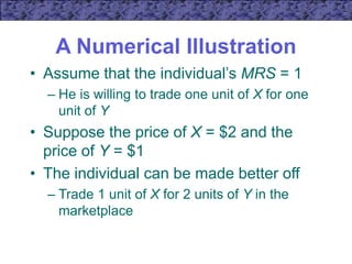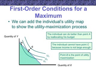3) A numerical example illustrates this principle using indifference curves and budget constraints. The consumer maximizes utility at the point of tangency between the indifference curve and budget line.

1. Chapter 4
UTILITY MAXIMIZATION
AND CHOICE
Copyright ©2002 by South-Western, a division of Thomson Learning. All rights reserved.
MICROECONOMIC THEORY
BASIC PRINCIPLES AND EXTENSIONS
EIGHTH EDITION
WALTER NICHOLSON

2. Complaints about Economic
Approach
• No real individuals make the kinds of
“lightning calculations” required for utility
maximization
• The utility-maximization model predicts
many aspects of behavior even though
no one carries around a computer with
his utility function programmed into it

3. Complaints about Economic
Approach
• The economic model of choice is
extremely selfish because no one has
solely self-centered goals
• Nothing in the utility-maximization
model prevents individuals from deriving
satisfaction from “doing good”

4. Optimization Principle
• To maximize utility, given a fixed amount
of income to spend, an individual will buy
the goods and services:
– that exhaust his or her total income
– for which the psychic rate of trade-off
between any goods (the MRS) is equal to
the rate at which goods can be traded for
one another in the marketplace

5. A Numerical Illustration
• Assume that the individual’s MRS = 1
– He is willing to trade one unit of X for one
unit of Y
• Suppose the price of X = $2 and the
price of Y = $1
• The individual can be made better off
– Trade 1 unit of X for 2 units of Y in the
marketplace

6. The Budget Constraint
• Assume that an individual has I dollars
to allocate between good X and good Y
PXX + PYY  I
Quantity of X
Quantity of Y The individual can afford
to choose only combinations
of X and Y in the shaded
triangle
Y
P
I
If all income is spent
on Y, this is the amount
of Y that can be purchased
X
P
I
If all income is spent
on X, this is the amount
of X that can be purchased

7. First-Order Conditions for a
Maximum
• We can add the individual’s utility map
to show the utility-maximization process
Quantity of X
Quantity of Y
U1
A
The individual can do better than point A
by reallocating his budget
U3
C
The individual cannot have point C
because income is not large enough
U2
B
Point B is the point of utility
maximization

8. First-Order Conditions for a
Maximum
• Utility is maximized where the indifference
curve is tangent to the budget constraint
Quantity of X
Quantity of Y
U2
B
constraint
budget
of
slope
Y
X
P
P


constant
curve
ce
indifferen
of
slope


U
dX
dY
MRS
dX
dY
P
P
U
Y
X


 constant
-

9. Second-Order Conditions for a
Maximum
• The tangency rule is only necessary but
not sufficient unless we assume that MRS
is diminishing
– if MRS is diminishing, then indifference curves
are strictly convex
• If MRS is not diminishing, then we must
check second-order conditions to ensure
that we are at a maximum

10. Second-Order Conditions for a
Maximum
• The tangency rule is only necessary but
not sufficient unless we assume that MRS
is diminishing
Quantity of X
Quantity of Y
U1
B
U2
A
There is a tangency at point A,
but the individual can reach a higher
level of utility at point B

11. Corner Solutions
• In some situations, individuals’ preferences
may be such that they can maximize utility
by choosing to consume only one of the
goods
Quantity of X
Quantity of Y U2
U1 U3
A
Utility is maximized at point A
At point A, the indifference curve
is not tangent to the budget constraint

12. The n-Good Case
• The individual’s objective is to maximize
utility = U(X1,X2,…,Xn)
subject to the budget constraint
I = P1X1 + P2X2 +…+ PnXn
• Set up the Lagrangian:
L = U(X1,X2,…,Xn) + (I-P1X1- P2X2-…-PnXn)

13. The n-Good Case
• First-order conditions for an interior
maximum:
L/X1 = U/X1 - P1 = 0
L/X2 = U/X2 - P2 = 0
•
•
•
L/Xn = U/Xn - Pn = 0
L/ = I - P1X1 - P2X2 - … - PnXn = 0

14. Implications of First-Order
Conditions
• For any two goods,
j
i
j
i
P
P
X
U
X
U





/
/
• This implies that at the optimal
allocation of income
j
i
j
i
P
P
X
X
MRS 
)
for
(

15. Interpreting the Lagrangian
Multiplier
•  is the marginal utility of an extra dollar
of consumption expenditure
– the marginal utility of income
n
n
P
X
U
P
X
U
P
X
U 










/
...
/
/
2
2
1
1
n
X
X
X
P
MU
P
MU
P
MU n




 ...
2
1
2
1

16. Interpreting the Lagrangian
Multiplier
• For every good that an individual buys,
the price of that good represents his
evaluation of the utility of the last unit
consumed
– how much the consumer is willing to pay
for the last unit

 i
X
i
MU
P

17. Corner Solutions
• When corner solutions are involved, the
first-order conditions must be modified:
L/Xi = U/Xi - Pi  0 (i = 1,…,n)
• If L/Xi = U/Xi - Pi < 0 then Xi = 0
• This means that





 i
X
i
i
MU
X
U
P
/
– Any good whose price exceeds its marginal
value to the consumer will not be purchased

18. Cobb-Douglas Demand
Functions
• Cobb-Douglas utility function:
U(X,Y) = XY
• Setting up the Lagrangian:
L = XY + (I - PXX - PYY)
• First-order conditions:
L/X = X-1Y - PX = 0
L/Y = XY-1 - PY = 0
L/ = I - PXX - PYY = 0

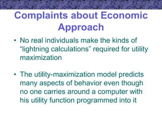
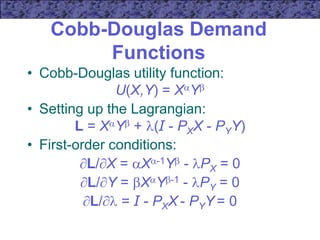
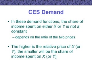
19. Cobb-Douglas Demand
Functions
• First-order conditions imply:
Y/X = PX/PY
• Since  +  = 1:
PYY = (/)PXX = [(1- )/]PXX
• Substituting into the budget constraint:
I = PXX + [(1- )/]PXX = (1/)PXX

20. Cobb-Douglas Demand
Functions
• Solving for X yields
• Solving for Y yields
X
P
X
I


*
Y
P
Y
I


*
• The individual will allocate  percent of
his income to good X and  percent of
his income to good Y

21. Cobb-Douglas Demand
Functions
• The Cobb-Douglas utility function is
limited in its ability to explain actual
consumption behavior
– the share of income devoted to particular
goods often changes in response to
changing economic conditions
• A more general functional form might be
more useful in explaining consumption
decisions

22. CES Demand
• Assume that  = 0.5
U(X,Y) = X0.5 + Y0.5
• Setting up the Lagrangian:
L = X0.5 + Y0.5 + (I - PXX - PYY)
• First-order conditions:
L/X = 0.5X-0.5 - PX = 0
L/Y = 0.5Y-0.5 - PY = 0
L/ = I - PXX - PYY = 0

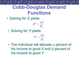
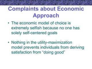
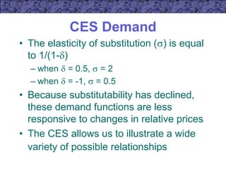
23. CES Demand
• This means that
(Y/X)0.5 = Px/PY
• Substituting into the budget constraint,
we can solve for the demand functions:
]
1
[
*
Y
X
X
P
P
P
X


I
]
1
[
*
X
Y
Y
P
P
P
Y


I

24. CES Demand
• In these demand functions, the share of
income spent on either X or Y is not a
constant
– depends on the ratio of the two prices
• The higher is the relative price of X (or
Y), the smaller will be the share of
income spent on X (or Y)

25. CES Demand
• If  = -1,
U(X,Y) = X-1 + Y-1
• First-order conditions imply that
Y/X = (PX/PY)0.5
• The demand functions are
]
1
[
* 5
.
0










X
Y
X
P
P
P
X
I
]
1
[
* 5
.
0










Y
X
Y
P
P
P
Y
I

26. CES Demand
• The elasticity of substitution () is equal
to 1/(1-)
– when  = 0.5,  = 2
– when  = -1,  = 0.5
• Because substitutability has declined,
these demand functions are less
responsive to changes in relative prices
• The CES allows us to illustrate a wide
variety of possible relationships

27. Indirect Utility Function
• It is often possible to manipulate first-
order conditions to solve for optimal
values of X1,X2,…,Xn
• These optimal values will depend on the
prices of all goods and income
•
•
•
X*n = Xn(P1,P2,…,Pn, I)
X*1 = X1(P1,P2,…,Pn,I)
X*2 = X2(P1,P2,…,Pn,I)

28. Indirect Utility Function
• We can use the optimal values of the Xs
to find the indirect utility function
maximum utility = U(X*1,X*2,…,X*n)
• Substituting for each X*i we get
maximum utility = V(P1,P2,…,Pn,I)
• The optimal level of utility will depend
indirectly on prices and income
– If either prices or income were to change,
the maximum possible utility will change

29. Indirect Utility in the Cobb-
Douglas
• If U = X0.5Y0.5, we know that
x
P
X
2
I

*
Y
P
Y
2
I

*
• Substituting into the utility function, we get
5
0
5
0
5
0
5
0
2
2
2 .
.
.
.
utility
maximum
Y
X
Y
X P
P
P
P
I
I
I



















30. Expenditure Minimization
• Dual minimization problem for utility
maximization
– allocating income in such a way as to achieve
a given level of utility with the minimal
expenditure
– this means that the goal and the constraint
have been reversed

31. Expenditure level E2 provides just enough to reach U1
Expenditure Minimization
Quantity of X
Quantity of Y
U1
Expenditure level E1 is too small to achieve U1
Expenditure level E3 will allow the
individual to reach U1 but is not the
minimal expenditure required to do so
A
• Point A is the solution to the dual problem

32. Expenditure Minimization
• The individual’s problem is to choose
X1,X2,…,Xn to minimize
E = P1X1 + P2X2 +…+PnXn
subject to the constraint
U1 = U(X1,X2,…,Un)
• The optimal amounts of X1,X2,…,Xn will
depend on the prices of the goods and
the required utility level

33. Expenditure Function
• The expenditure function shows the
minimal expenditures necessary to
achieve a given utility level for a particular
set of prices
minimal expenditures = E(P1,P2,…,Pn,U)
• The expenditure function and the indirect
utility function are inversely related
– both depend on market prices but involve
different constraints

34. Expenditure Function from
the Cobb-Douglas
• Minimize E = PXX + PYY subject to
U’=X0.5Y0.5 where U’ is the utility target
• The Lagrangian expression is
L = PXX + PYY + (U’ - X0.5Y0.5)
• First-order conditions are
L/X = PX - 0.5X-0.5Y0.5 = 0
L/Y = PY - 0.5X0.5Y-0.5 = 0
L/ = U’ - X0.5Y0.5 = 0

35. Expenditure Function from
the Cobb-Douglas
• These first-order conditions imply that
PXX = PYY
• Substituting into the expenditure function:
E = PXX* + PYY* = 2PXX*
Solving for optimal values of X* and Y*:
X
P
E
X
2

*
Y
P
E
Y
2

*

36. Expenditure Function from
the Cobb-Douglas
• Substituting into the utility function, we
can get the indirect utility function
5
0
5
0
5
0
5
0
2
2
2 .
.
.
.
'
Y
X
Y
X P
P
E
P
E
P
E
U 

















• So the expenditure function becomes
E = 2U’PX
0.5PY
0.5

37. Important Points to Note:
• To reach a constrained maximum, an
individual should:
– spend all available income
– choose a commodity bundle such that the
MRS between any two goods is equal to the
ratio of the goods’ prices
• the individual will equate the ratios of marginal utility
to price for every good that is actually consumed

38. Important Points to Note:
• Tangency conditions are only first-order
conditions
– the individual’s indifference map must exhibit
diminishing MRS
– the utility function must be strictly quasi-
concave
• Tangency conditions must also be modified
to allow for corner solutions
– ratio of marginal utility to price will be lower for
goods that are not purchased

39. Important Points to Note:
• The individual’s optimal choices implicitly
depend on the parameters of his budget
constraint
– choices observed will be implicit functions of
prices and income
– utility will also be an indirect function of prices
and income

40. Important Points to Note:
• The dual problem to the constrained utility-
maximization problem is to minimize the
expenditure required to reach a given utility
target
– yields the same optimal solution as the primary
problem
– leads to expenditure functions in which
spending is a function of the utility target and
prices