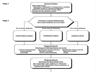
CONJOINT ANALYSIS
By: GROUP -10
Anmol Sahni Chinmay Jagga
Dhruval Dholakia Mayank Sharma
Madhusudan Partani Mudita Maheshwari
Neha Arya Neha Kasturia
Radhika Gupta Shivi Aggarwal
What is ConjointAnalysis?
• Definition : Conjoint Analysis is a multivariate technique
developed specifically to understand how respondents
develop preferences for any type of object.
• Based on the premise that consumers evaluate the value of
an object by combining the separate amounts of value
provided by each attribute.
• Also known as :
o Multi-attribute Compositional Modelling
o Discrete Choice Modelling
o Stated Preference Research
Important Terminology
• Factor: Independent variable the researcher manipulates that
represents a specific attribute
• Level: Specific non-metric value describing a factor. Each factor
must be represented by two or more levels.
• Profile : Combination of all possible levels of factors. For ex: 3
factors with 2 levels each will create (2x2x2) i.e. 8 profiles.
• Utility: An individual’s subjective preference judgment
representing the holistic value or worth of a specific object.
• Part-worth: Estimate from conjoint analysis of the overall
preference or utility associated with each level of each factor
used to define the product or service
Why use Conjoint Analysis ?
Different Perspectives, Different Goals
• Buyers want all of the most desirable features at lowest
possible price
• Sellers want to maximize profits by:
1) minimizing costs of providing features
2) providing products that offer greater overall value than the
competition
Conjoint Analysis is concerned with understanding
how people make choices between products or services or a combination of
product and service, so that businesses can design new products or
services that better meet customers’ underlying needs.
Attributes andLevels
• Attribute: An attribute is a general feature of a
product or service – say size, colour, speed, delivery
time.
• Level: Each attribute is then made up of specific
levels. So for the attribute colour, levels might be red,
green, blue and so on.
Understanding Conjoint Analysis
• Conjoint analysis takes these attribute and level
descriptions of product/services by asking people to
make a number of choices between different products.
Example :
Would you choose phone A or phone B?
Phone A Phone B
Weight 200g 120g
Battery Life 21 hours 10 hours
Price Rs 5000 Rs 8000
• Researcher can work out numerically (from the responses)
how valuable each of the levels is relative to the others
around it – this value is known as the utility of the level.
• We can also compare across attributes to see which attributes
make have the greatest impact in making a choice.
Utility value for each level of
Weight
40
50
35
25
15
40g 80g 120g 160g 200g
Relative importance of attributes
45%
35%
20%
Weight Price Battery
Company’sObjective
How our product/service compares to our
competitors and how we can best optimise the
value we give to the customer?
By Conjoint analysis :
We can total up the utility value our product is
giving the customer and compare it to the
value for the competition
Example (cont.) :
Note : Utility values are in brackets. A lower price has a
higher utility.
Phone A
(Our Product)
Phone B
(Competitor’s
Product)
Weight 200g (15) 120g (35)
Battery Life 21 hours (15) 10 hours (10)
Price Rs 5000 (25) Rs 8000 (15)
Total Utility 55 60
Estimating Part-worth
• Part-worths are calculated by using:
– Multiple Regression with dummy variables
– ANOVA
– Multinomial logit Models
• Calculations are done for each respondent
separately
DeterminingAttribute Importance
• Importance of a factor is represented by the
range of its levels (difference between highest
and lowest values) divided by the sum of the
ranges across all the factors.
• This provides relative importance of each
attribute based on the range of its part-worth
estimates.
Assessing PredictiveAccuracy
To examine the ability of the model to predict the
actual choices of respondents:
• We predict the preference order by summing the
part-worths for the profiles and then rank-
ordering the resulting scores
• Comparing the predictive preference order to the
respondent’s actual preference order assesses
predictive accuracy
Designing profiles
Selecting and defining factors and levels
Its important as it determines
-> effectiveness of the profiles in the task
-> accuracy of results
-> managerial relevance
Generalcharacteristicsof factors
1) Communicable
-> sensory and
multimedia effects
included
2) Actionable
-> should be capable of
being put into
practice
Issues in defining factors
• Number of factors
• Inter attribute correlation
• Unique role of price
Specification issues regarding
levels
1) Number and balance of levels
2) Range of levels
• Two major key decisions involved in
specifying the model are as follows:-
1) Specifying the composition rule used:-
a) Additive rule
b) Interactive rule
2) Selecting the type of part worth relation
ships
a) Linear model
b) Quadratic model
c) Separate part worth model
0
1
2
3
4
Level
Prefernce
0
1
2
3
4
0 2 4
Preferenc
e
0
1
2
3
4
5
 Linear model
Quadratic model

 Separate part worth model
Designing a conjoint analysis
experiment
Stage 1:Objectivesof the conjoint
analysis
• To determine the contributions of predictor
variables and their levels in determination
of consumer preference
• To establish a valid model of consumer
judgments
Requirementsfor a successful conjointanalysis
• Defining the total utility of the object
• all attributes that potentially create or detract from
the overall utility of the product or service should
be included
• Specifying the determinant factors
• include the factors that best differentiate between
the objects
Stage 3:Assumptions Of ConjointAnalysis
 The product is a bundle of attributes.
 Utility of a product is a simple function of the utilities
of the attributes.
 Utility predicts behaviour (i.e., purchases).
Least restrictive set of statistical assumptions but highly
critical conceptual assumptions.
Stage 4: Estimating the ConjointModel
• Traditional Estimation Approaches:
– For non metric preference measures:
» MONANOVA, LINMAP
– For metric preference measures:
» Multiple regression with dummy variables
– For more complex consumer preference
measures:
» Logit model and its extensions
• Extension of Basic Estimation Process
– Bayesian Estimation
– Incorporation of additional variables reflecting
characteristics of the individuals
Stage 5: Interpretingthe results
• Generally done at disaggregate level
• For aggregate behavior, such as market share,
aggregate analysis more accurate.
• Two main things considered in interpretation
– Examining the estimated part-worth
• Magnitude and pattern of part-worth for each factor
• Higher the part-worth, higher the impact on overall utility
– Relative importance of attributes
• Factor with greatest range of part-woths has greatest
contribution to overall utility.
ManagerialImplications
Define the object with the optimal
combination of features
Predict market shares of different
objects with different sets of features
Isolate groups of customers who place
differing importance’s on different
features
Identify marketing opportunities by
exploring the market potential for
feature combos not currently available
Show the relative contributions of each
attribute and each level to the overall
evaluation of the object
Types Of Analysis
AggregateAnalysis
• Used to generally determine
– average part worth of each attribute level across
the entire sample of respondents
• This usually helps in determining the
– The importance of each attribute
– The desired level of each attribute
Segment Analysis
• In most marketing situations, strategies are
based on customer segments
• Cluster analysis used to produce “benefit
segments”
• Clusters are formed to group respondent such
that segments have similar within a segment
and different across segments
ScenarioSimulations
• Conjoint Analysis also helps researchers to
simulate various competitive scenarios
• Scenarios are used to estimate how
respondents react to various scenarios
• It is used to understand how the set of
respondents would choose among a specified
set of profiles
Comparingconjoint analysis with other
multivariatemodels
• Its decompositional nature
• Specification of the variate
• The fact that estimates can be made at
individual level
• Its flexibility in terms of relationships
between dependent and independent
variables
Compositionalvsdecompositional
techniques
• In compositional models the researcher collects
ratings from the respondent on many product
characteristics and then relates theses ratings to
the to some overall preference rating to develop
a predictive model
• Conjoint analysis a type of decompositional
model, differs in that the researcher needs to
know only respondents overall preference for a
profile.
Specifyingthe conjointvariate
• Conjoint analysis employs a variate quite similar in
form to what is used in other multivariate techniques.
• The conjoint variate is a linear combination of effects
of the independent variables (levels of each factor) on
a dependent variable.
• The important difference is that in the conjoint
variate the researcher specifies both the independent
variables (factors) and their values (levels).
Separatemodels for eachindividual
• Conjoint analysis can be carried out at the
individual level
• other multivariate methods use each
respondent’s measures as a single
observation and then perform the analysis
using all respondents simultaneously.
Flexibilityin types of relationships
• Conjoint analysis not limited in types of
relationships required between the dependent
and independent variables
• Most dependence methods assume that a
linear relationship exists
• Conjoint analysis can easily handle non linear
relationships as well
Conjoint Analysis

Conjoint Analysis

  • 1.
    CONJOINT ANALYSIS By: GROUP-10 Anmol Sahni Chinmay Jagga Dhruval Dholakia Mayank Sharma Madhusudan Partani Mudita Maheshwari Neha Arya Neha Kasturia Radhika Gupta Shivi Aggarwal
  • 2.
    What is ConjointAnalysis? •Definition : Conjoint Analysis is a multivariate technique developed specifically to understand how respondents develop preferences for any type of object. • Based on the premise that consumers evaluate the value of an object by combining the separate amounts of value provided by each attribute. • Also known as : o Multi-attribute Compositional Modelling o Discrete Choice Modelling o Stated Preference Research
  • 3.
    Important Terminology • Factor:Independent variable the researcher manipulates that represents a specific attribute • Level: Specific non-metric value describing a factor. Each factor must be represented by two or more levels. • Profile : Combination of all possible levels of factors. For ex: 3 factors with 2 levels each will create (2x2x2) i.e. 8 profiles. • Utility: An individual’s subjective preference judgment representing the holistic value or worth of a specific object. • Part-worth: Estimate from conjoint analysis of the overall preference or utility associated with each level of each factor used to define the product or service
  • 4.
    Why use ConjointAnalysis ? Different Perspectives, Different Goals • Buyers want all of the most desirable features at lowest possible price • Sellers want to maximize profits by: 1) minimizing costs of providing features 2) providing products that offer greater overall value than the competition Conjoint Analysis is concerned with understanding how people make choices between products or services or a combination of product and service, so that businesses can design new products or services that better meet customers’ underlying needs.
  • 5.
    Attributes andLevels • Attribute:An attribute is a general feature of a product or service – say size, colour, speed, delivery time. • Level: Each attribute is then made up of specific levels. So for the attribute colour, levels might be red, green, blue and so on.
  • 6.
    Understanding Conjoint Analysis •Conjoint analysis takes these attribute and level descriptions of product/services by asking people to make a number of choices between different products. Example : Would you choose phone A or phone B? Phone A Phone B Weight 200g 120g Battery Life 21 hours 10 hours Price Rs 5000 Rs 8000
  • 7.
    • Researcher canwork out numerically (from the responses) how valuable each of the levels is relative to the others around it – this value is known as the utility of the level. • We can also compare across attributes to see which attributes make have the greatest impact in making a choice. Utility value for each level of Weight 40 50 35 25 15 40g 80g 120g 160g 200g Relative importance of attributes 45% 35% 20% Weight Price Battery
  • 8.
    Company’sObjective How our product/servicecompares to our competitors and how we can best optimise the value we give to the customer? By Conjoint analysis : We can total up the utility value our product is giving the customer and compare it to the value for the competition
  • 9.
    Example (cont.) : Note: Utility values are in brackets. A lower price has a higher utility. Phone A (Our Product) Phone B (Competitor’s Product) Weight 200g (15) 120g (35) Battery Life 21 hours (15) 10 hours (10) Price Rs 5000 (25) Rs 8000 (15) Total Utility 55 60
  • 10.
    Estimating Part-worth • Part-worthsare calculated by using: – Multiple Regression with dummy variables – ANOVA – Multinomial logit Models • Calculations are done for each respondent separately
  • 11.
    DeterminingAttribute Importance • Importanceof a factor is represented by the range of its levels (difference between highest and lowest values) divided by the sum of the ranges across all the factors. • This provides relative importance of each attribute based on the range of its part-worth estimates.
  • 12.
    Assessing PredictiveAccuracy To examinethe ability of the model to predict the actual choices of respondents: • We predict the preference order by summing the part-worths for the profiles and then rank- ordering the resulting scores • Comparing the predictive preference order to the respondent’s actual preference order assesses predictive accuracy
  • 13.
    Designing profiles Selecting anddefining factors and levels Its important as it determines -> effectiveness of the profiles in the task -> accuracy of results -> managerial relevance
  • 14.
    Generalcharacteristicsof factors 1) Communicable ->sensory and multimedia effects included 2) Actionable -> should be capable of being put into practice
  • 15.
    Issues in definingfactors • Number of factors • Inter attribute correlation • Unique role of price
  • 16.
    Specification issues regarding levels 1)Number and balance of levels 2) Range of levels
  • 17.
    • Two majorkey decisions involved in specifying the model are as follows:- 1) Specifying the composition rule used:- a) Additive rule b) Interactive rule 2) Selecting the type of part worth relation ships a) Linear model b) Quadratic model c) Separate part worth model
  • 18.
    0 1 2 3 4 Level Prefernce 0 1 2 3 4 0 2 4 Preferenc e 0 1 2 3 4 5 Linear model Quadratic model   Separate part worth model
  • 19.
    Designing a conjointanalysis experiment
  • 22.
    Stage 1:Objectivesof theconjoint analysis • To determine the contributions of predictor variables and their levels in determination of consumer preference • To establish a valid model of consumer judgments
  • 23.
    Requirementsfor a successfulconjointanalysis • Defining the total utility of the object • all attributes that potentially create or detract from the overall utility of the product or service should be included • Specifying the determinant factors • include the factors that best differentiate between the objects
  • 24.
    Stage 3:Assumptions OfConjointAnalysis  The product is a bundle of attributes.  Utility of a product is a simple function of the utilities of the attributes.  Utility predicts behaviour (i.e., purchases). Least restrictive set of statistical assumptions but highly critical conceptual assumptions.
  • 25.
    Stage 4: Estimatingthe ConjointModel • Traditional Estimation Approaches: – For non metric preference measures: » MONANOVA, LINMAP – For metric preference measures: » Multiple regression with dummy variables – For more complex consumer preference measures: » Logit model and its extensions
  • 26.
    • Extension ofBasic Estimation Process – Bayesian Estimation – Incorporation of additional variables reflecting characteristics of the individuals
  • 27.
    Stage 5: Interpretingtheresults • Generally done at disaggregate level • For aggregate behavior, such as market share, aggregate analysis more accurate. • Two main things considered in interpretation – Examining the estimated part-worth • Magnitude and pattern of part-worth for each factor • Higher the part-worth, higher the impact on overall utility – Relative importance of attributes • Factor with greatest range of part-woths has greatest contribution to overall utility.
  • 28.
  • 29.
    Define the objectwith the optimal combination of features Predict market shares of different objects with different sets of features Isolate groups of customers who place differing importance’s on different features Identify marketing opportunities by exploring the market potential for feature combos not currently available Show the relative contributions of each attribute and each level to the overall evaluation of the object
  • 30.
  • 31.
    AggregateAnalysis • Used togenerally determine – average part worth of each attribute level across the entire sample of respondents • This usually helps in determining the – The importance of each attribute – The desired level of each attribute
  • 32.
    Segment Analysis • Inmost marketing situations, strategies are based on customer segments • Cluster analysis used to produce “benefit segments” • Clusters are formed to group respondent such that segments have similar within a segment and different across segments
  • 33.
    ScenarioSimulations • Conjoint Analysisalso helps researchers to simulate various competitive scenarios • Scenarios are used to estimate how respondents react to various scenarios • It is used to understand how the set of respondents would choose among a specified set of profiles
  • 34.
    Comparingconjoint analysis withother multivariatemodels • Its decompositional nature • Specification of the variate • The fact that estimates can be made at individual level • Its flexibility in terms of relationships between dependent and independent variables
  • 35.
    Compositionalvsdecompositional techniques • In compositionalmodels the researcher collects ratings from the respondent on many product characteristics and then relates theses ratings to the to some overall preference rating to develop a predictive model • Conjoint analysis a type of decompositional model, differs in that the researcher needs to know only respondents overall preference for a profile.
  • 36.
    Specifyingthe conjointvariate • Conjointanalysis employs a variate quite similar in form to what is used in other multivariate techniques. • The conjoint variate is a linear combination of effects of the independent variables (levels of each factor) on a dependent variable. • The important difference is that in the conjoint variate the researcher specifies both the independent variables (factors) and their values (levels).
  • 37.
    Separatemodels for eachindividual •Conjoint analysis can be carried out at the individual level • other multivariate methods use each respondent’s measures as a single observation and then perform the analysis using all respondents simultaneously.
  • 38.
    Flexibilityin types ofrelationships • Conjoint analysis not limited in types of relationships required between the dependent and independent variables • Most dependence methods assume that a linear relationship exists • Conjoint analysis can easily handle non linear relationships as well

Editor's Notes

  • #5 Conjoint Analysis is concerned with understanding how people make choices between products or services or a combination of product and service, so that businesses can design new products or services that better meet customers’ underlying needs.
  • #8 In this instance we can see that for this customer, the optimum weight is 80g. 40g is too light and more than 80g is too heavy. In designing a mobile phone for this customer therefore, we can see that there is no benefit in spending development money to bring the weight of the phone below 80g. Also, we see that getting the weight right is more than twice as important as looking at the battery life.
  • #10 In this example we are 5 utility points behind the competition. If we reduced the weight of the phone to 160g we would gain 10 utility points which would mean we would expect to be chosen over the competition. Alternatively, we could to reduce the price a little to have the same impact.
  • #32 Although one of the virtues of conjoint is its separate treatment of each individual, the most common first interpretation step is to compute average part worth of each attribute level across the entire sample of respondents to give the analyst an overall feeling for which attributes are generally important and what is the most desired level of each.
  • #33 The averages are useful, convenient, and easy to understand summary measure. In most marketing situations, however, strategies are based on customer segments. There are numbers of alternative approaches to derive segments. Since the value system can be derived for each respondent, a cluster analysis can be used to produce “benefit segments”. Idea behind clusters is to group respondent such that segments have similar within a segment and different across segments. Instead of cluster analysis one may use latent class approach to derive statistically meaningful segments. Another alternative is to look at predefined group of customers based on some prior knowledge about them. For example, current versus prospective customers or heavy versus light volume buyers.
  • #34 Conjoint Analysis also helps researchers to simulate various competitive scenarios and then estimate how the respondents would react to each scenario. A conjoint simulation is an attempt to understand how the set of respondents would choose among a specified set of profiles. The process provides the researcher with the ability to utilize the estimated parts worth in evaluating a number of scenarios consisting of a number of possible combinations of the profiles.