Download to read offline


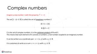
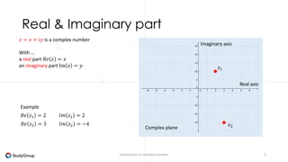
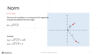
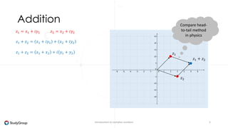
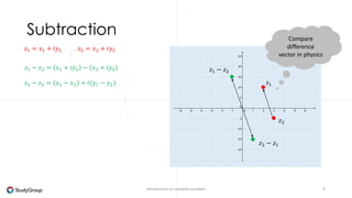
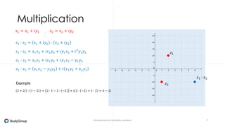
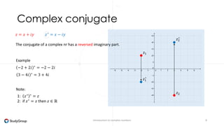
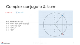
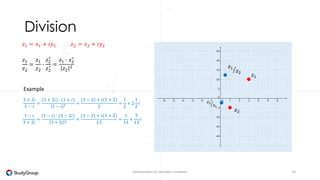


Complex numbers are numbers that consist of a real part and an imaginary part. The imaginary part is represented by the imaginary unit i, where i^2 = -1. The set of complex numbers C is the cartesian product of the real numbers R and imaginary numbers I. A complex number z can be written as z = x + iy, where x and y are real numbers representing the real and imaginary parts. Operations like addition, subtraction, multiplication and division can be performed with complex numbers by treating i as a variable and applying the standard rules of arithmetic.