Download to read offline
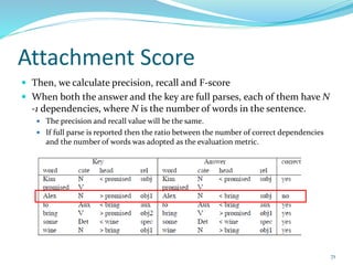
![Average precision and recall
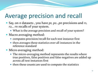
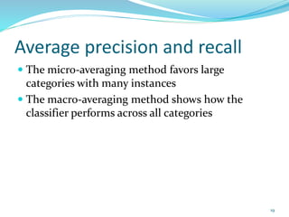
Say, your system has the following performance on two
datasets
tp1 = 10, fp1 = 5, fn1 = 3, p = 66.67, r = 76.92
tp2 = 20, fp2 = 4, fn2 = 5, p = 83.33, r = 80.00
Macro p = (66.67 + 83.33)/2 = 75
Macro r = (76.92+80.00)/2 = 78.46
Micro p = (10+20)/[(10+20)+(5+4)]= 76.92
Micro r = (10+20)/[(10+20)+(3+5)] = 78.94
18](https://image.slidesharecdn.com/commonevaluationmeasuresinnlpandir-210817020305/85/Common-evaluation-measures-in-NLP-and-IR-18-320.jpg)
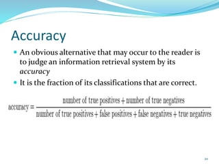
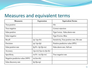
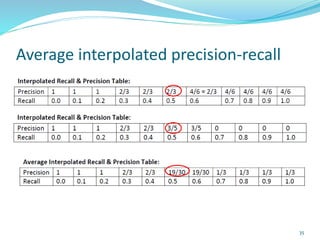
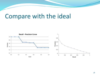
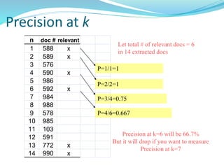
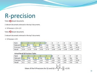
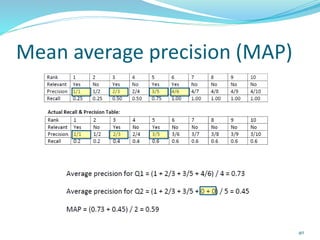
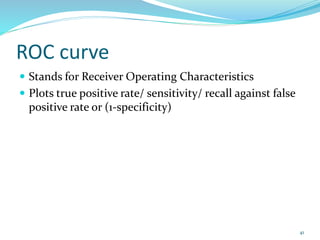
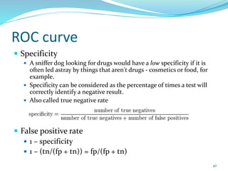

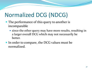
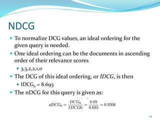

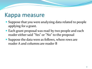
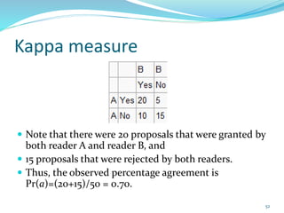
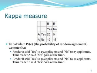
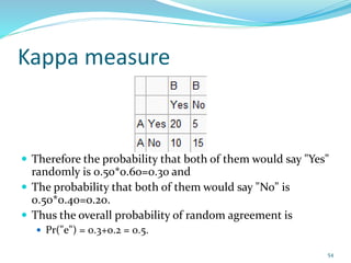
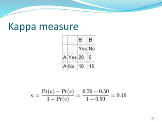
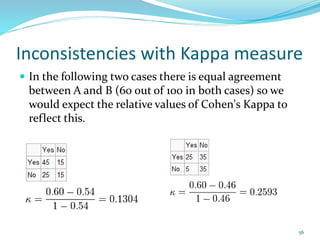
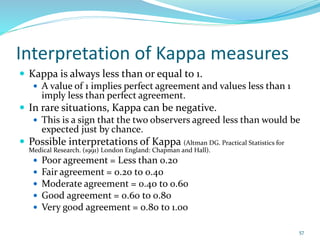
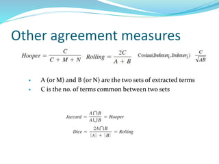

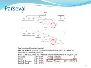
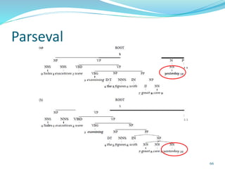

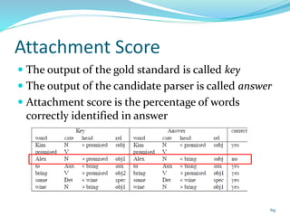
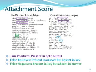


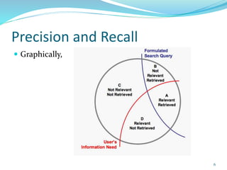
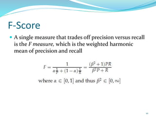
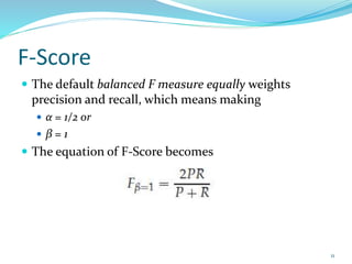
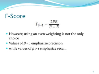
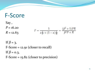
This document discusses various evaluation measures used in information retrieval and natural language processing. It describes precision, recall, and the F1 score as fundamental measures for unranked retrieval sets. It also covers averaged precision and recall, accuracy, novelty and coverage ratios. For ranked retrieval sets, it discusses recall-precision graphs, interpolated recall-precision, precision at k, R-precision, ROC curves, and normalized discounted cumulative gain (NDCG). The document also discusses agreement measures like Kappa statistics and parses evaluation measures like Parseval and attachment scores.