Download to read offline


![6 CHAPTER 1. INTRODUCTION
at transrating to the same video format, with particular emphasis on MPEG-2, we
limit our discussion here to this case, i.e., to what is known as transrating.
1.1 Transrating goals
Transrating to the same video format is usually done in order to reduce the bit-rate of
the encoded stream, while preserving the highest possible quality of the rate-reduced
video. This goal can be set as to achieve the same subjective quality in the entire
frame or mostly in regions that can be defined as more informative.
If we are talking about simultaneous transrating of several or many channels that
have to be transmitted over the same Constant Bit Rate (CBR) channel, the goal
can be set as to increase the mean quality of every sub-channel by taking advantage
of non-constant sub-channel usage by other programs [1].
1.2 Transrating approaches
For a specific bit-stream, bit-rate reduction can be achieved by:
1. Frame-rate reduction [2]. Video is usually encoded using temporal prediction
techniques, so that not all types of frames can have their rates reduced with-
out introducing additional errors in other frames. The problems of prediction
re-estimation and total error minimization over all frames have to be taken
into account.However, if talking about B-frames dropping only, no motion re-
estimation problem appear.
2. Requantization (increasing quantization step) or/and by discarding Discrete
Cosine Transform (DCT) coefficients [3, 4, 5, 6, 7, 8, 9, 10]. This issue will be](https://image.slidesharecdn.com/13642942-120715025949-phpapp01/85/Michael_Lavrentiev_Trans-trating-PDF-14-320.jpg)
![1.2. TRANSRATING APPROACHES 7
discussed in detail in the sequel.
3. Spatial resolution reduction using frame size rescaling (via decimation) [11, 12,
13]. Spatial resolution reduction can be applied in the DCT domain. Still,
prediction re-estimation and error propagation are to be faced.
4. Some other means like picture cropping [14]. If one can define the importance
of each part of the image, picture cropping that leaves the most important parts
with total bit-rate under a given constraint can be provided. However, these
methods need side information about different parts of the video sequence and
their relative importance.
In this work we consider only methods of requantization or elimination of DCT coeffi-
cients without frame dropping, cropping or re-scaling. These methods can be applied
without any additional information about picture content and may be done without
prediction re-estimation, which is the most computational intensive operation.
1.2.1 DCT coefficients modification
Several transrating methods were recently discussed in the literature [3, 8, 15, 16,
17]. The straightforward approach is to fully decode the sequence, and to encode it
by the same encoder but with more severe constraints. However, this approach is
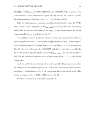
computational expensive, and also introduces requantization errors to the full extent.
This is because re-encoding depends on the initial encoding, but does not take it
into account in any way. Alternatively, using decisions made in the initial encoding
process may help in minimizing the computational load, as well in error reduction. As
discussed by [8],[15] transrating approaches can be coarsely classified by the methods](https://image.slidesharecdn.com/13642942-120715025949-phpapp01/85/Michael_Lavrentiev_Trans-trating-PDF-15-320.jpg)
![8 CHAPTER 1. INTRODUCTION
used for building the transrating architectures. At the upper level they can be divided
as follows:
1. Re-encoding using the original motion vectors and coding decisions such as
Macro Block (MB) types, quantization weighting matrix, Group Of Pictures
(GOP) and slice (group of MBs) structures, motion vectors, etc. [3], [8].
2. Re-encoding using the original motion vectors information but new coding de-
cisions [8]. For example, in B-pictures the prediction type can be changed from
bi-directional to forward or backward only, with a proper update of the mo-
tion vectors, but the information about the original prediction area can help in
reducing the motion estimation complexity.
Bit-rate reduction in each of the above classes is achieved by one of the following
means:
1. Discarding high frequency DCT coefficients [8, 16, 17]. In this method, de-
coding up to the point (inclusive) of inverse Variable Length Coding (VLC) is
performed. At this point the transcoder has exact information about MB bit
allocation, and can easily calculate the bit-rate produced after it changes the
bit-stream. In the case of discarding of the last coefficients in zig-zag scan, the
transcoder can calculate the gain in bit-rate reduction by simply reducing the
length of the corresponding VLC words from the input MB bit-rate occupation.
In the case of dropping non-zero coefficients from the middle of the zig-zag
scan, the VLC lookup tables need to be used to find the change in bit-rate. The
rate-distortion optimization problem can be solved as described in the sequel
in section 4.2. One more aspect of this method is that the introduced distor-
tion is directly obtained from the discarded coefficients and hence simplifies the](https://image.slidesharecdn.com/13642942-120715025949-phpapp01/85/Michael_Lavrentiev_Trans-trating-PDF-16-320.jpg)
![1.2. TRANSRATING APPROACHES 9
calculations.
2. Requantization by just increasing the quantization step [8]. This is actually
a more complex scheme than the previous one. After inverse VLC, the DCT
coefficients need to be recovered, using inverse quantization. Bit-rate reduction
is achieved by quantizing the coefficients with a larger quantizer step. The
assumption is that this will produce an error that is more equally distributed
among all DCT coefficients than by discarding some of them. In such a case
there is no easy way to predict the introduced error and the resulting bit-rate.
1.2.2 Open-loop vs. closed-loop transrating
When talking about transrating complexity and robustness, open-loop and closed-
loop transrating have to be considered. Open-loop transrating refers to transrating
of the bit-stream on a frame-by-frame basis, without taking into account the changes
done to previously transcoded frames. It is the fastest approach, but it leads to a
continuously decreasing quality in each Group Of Pictures (GOP), because in MPEG,
as well as in many others video encoding techniques, frame prediction is used, and
only frame residuals with prediction parameters are actually sent. As an alternative,
closed-loop transrating was proposed in [3], [9]. The idea is to add the information re-
moved by the transrating process in a given frame to the data of the next dependent
frames. Alternatively, it can be seen as compensating the error introduced during
transrating. The reduction in error propagation is of utmost importance because
differential encoding is used in most video encoding systems due to its efficiency.
However, there is the problem that the error propagation depends on motion predic-
tion. After intensive research in this area, it was found that if the only change one](https://image.slidesharecdn.com/13642942-120715025949-phpapp01/85/Michael_Lavrentiev_Trans-trating-PDF-17-320.jpg)
![10 CHAPTER 1. INTRODUCTION
wants to introduce is in the quantization step, all the computations for closed-loop
error compensation can also be done in the DCT domain [10],[18]. Of course, this
bring up a whole new set of problems: How to produce motion compensation in the
DCT domain [11]; what to do with skipped MBs; what additional changes in bit
stream structure have to be done if a change in the GOP structure is necessary (for
example, if the rate control provides no bits for the transmission of particular frame).
But the most important one is how to obtain the best possible quality at the required
output bit-rate.
1.2.3 HVS-based Adaptive Transrating
The quantification of the introduced distortion is typically done via the Mean-Squared-
Error (MSE). The problem with the MSE metric is that it is not always a good
indicator of picture quality. There is a general agreement that the Human Visual
System (HVS) properties have to be taken into account while encoding/transrating
of video sequences. The idea behind adaptive requantization is that distortion in a
macroblock may be masked in proportion to macroblock activity. Current encoders
apply adaptive quantization through video sequence analysis accounting for the HVS
characteristics. A standard simulation model known as TM (”Video Codec Test
Model”) is described in [7]. In this model the quantization steps are obtained by
multiplying a base quantization step by a weighting factor determined during the
encoding process. Since, according to [7], MB activities cannot be obtained from the
bit-stream, unless it is fully decoded to recover the picture, it is necessary to estimate
appropriate requantization parameters from the coded information.](https://image.slidesharecdn.com/13642942-120715025949-phpapp01/85/Michael_Lavrentiev_Trans-trating-PDF-18-320.jpg)
![1.2. TRANSRATING APPROACHES 11
1.2.4 Rate control
The main task of the transcoder is to achieve a certain bit-rate reduction. So, one of
the most important components of adaptive quantization schemes is a model for the
number of bits needed to code a macroblock for different values of the quantization
step. Such a model reduces the need to check all the possible quantization steps,
hence decreases the computational complexity of the transcoder.
The bit allocation and buffer control processes at the encoder produce base quan-
tization steps for each of the GOP, picture, slice and macroblock layers. Local quan-
tization step on slice or MB level and average quantization step over the picture,
obtained from coded data, well reflect the local activity and average activity, respec-
tively [1]. Methods proposed in [1],[19] are based on the idea of providing a ratio
between quantization steps at the different layers that are as close as possible to
those in the originally encoded stream. The idea of adaptive quantization is also used
in [20] to develop transrating in the DCT domain, based on analyzing a range of
macroblock coefficients values.
It is also a task of transcoding rate control to define the bit-allocation for every
frame in the GOP. Some algorithm also try to preserve the ratio of bit-allocations
provided by encoding procedure [21]. Other schemes are using the picture complexity,
which is defined as the product of the average quantizer step-size and the number
of bits generated, divided by some empirical constant [22, 23, 24, 25]. They provide
bit allocation according to frame complexities for the frames of the same type. The
results of those schemes have to be further changed to withstand the virtual buffer
constraints. In [26] an algorithm based on tracking virtual buffer fullness is proposed.
Those methods use the complexity instead of the variance of the block used by stan-
dard MPEG-2 TM5 rate control. The above frame-level rate-control schemes will be](https://image.slidesharecdn.com/13642942-120715025949-phpapp01/85/Michael_Lavrentiev_Trans-trating-PDF-19-320.jpg)
![12 CHAPTER 1. INTRODUCTION
described in details in section 2.2.
1.2.5 Relation between reconstruction error and bit-rate
According to [16], the DCT coefficients of difference frames are assumed to have a
Laplacian pdf (eq. 3.3). It is shown in [3] that if one assumes that the encoding bit-
rate is close to the entropy H of the quantized coefficients, then the bit-rate obtained
after requantization, by applying de-quantization (with quantization step q1 ) and
quantization with a new quantization step, q2 , has a step-like decreasing behavior as
function of q2 /q1 . At the same time the Peak Signal to Noise Ratio (PSNR) for a
given ”entropy step” is varying over the corresponding range of q2 /q1 , with a more
pronounced variation for small ratio values. Similar results were reported by [27] for
a Gaussian pdf. The work in [27] also provides the optimal requantization steps as
function of the initial quantization steps that achieve in simulations the best PSNR
for a given bit-rate reduction factor. In [27] no comparison with theoretical results
is provided. Those results were further extended by [23] for complexity reduction of
Lagrangian optimization in open-loop transrating. In [28] it is proposed to disable
requantization in the range up to twice the original quantization step, because it was
shown there that in this range there is the biggest degradation in PSNR, per bit. For
larger quantizer step sizes, the optimization problem was solved using a Lagrangian
optimization, as presented in section 4.2.
1.3 Organization of the Thesis
This thesis is organized as follows:
Chapter 2 covers existing transrating architectures, GOP-level bit-rate control](https://image.slidesharecdn.com/13642942-120715025949-phpapp01/85/Michael_Lavrentiev_Trans-trating-PDF-20-320.jpg)

![Chapter 2
Reference Transrating scheme
When building a transrating system, it is necessary to decide on its architecture, and
to develop a rate-control scheme. The merit of the final system is judged on the basis
of how good it meets the rate constraints, and how good is the video quality of the
transrated stream. However, the system complexity is also an important issue when
choosing a particular solution. Section 2.1 presents existing transrating architectures.
In section 2.2 different rate control schemes are described. In section 2.3 we propose a
simple complexity-based transrating scheme that will be used as a reference, to which
more advanced methods will be compared.
2.1 Transrating architectures
Following [3],the first, and the most straightforward transrating approach is Cascaded
Pixel Domain (CPD) transrating. It consist of a standard decoder and encoder, which
are applied one after another, as shown in Fig.2.1. The video is fully decoded and
then encoded to a new rate as if working on a source sequence. This scheme has the
15](https://image.slidesharecdn.com/13642942-120715025949-phpapp01/85/Michael_Lavrentiev_Trans-trating-PDF-23-320.jpg)
![16 CHAPTER 2. REFERENCE TRANSRATING SCHEME
Decoder Encoder
E VLD E Q−1 E IDCT E +j E - E DCT E
j Q2 E VLC E
1
T T c
Q−1
2
c c
side information E MC ' MEM IDCT
VLD/VLC - Variable Length Decoding / Coding
c
MC/ME - Motion Compensation / Estimation E+j
IDCT/DCT - Inverse/ Discrete Cosine Transform
MEM - Frame store memory buffer ME ' MEM '
Q−1 - Inverse first generation quantization
1
Q−1 /Q2 - Inverse / second generation quantization
2
Figure 2.1: Cascaded Pixel-domain Transrating scheme.
following disadvantages:
1. Using the decoded video as a source sequence that is re-encoded compounds the
encoding errors and the quality degrades more than with most other compressed-
domain schemes.
2. Motion estimation is the most computationally expensive part of the encoding
procedure. Since motion estimation was done already during initial encoding,
it could be re-used. However, in this scheme this information is not used at all.
3. Since the encoder includes a decoder in its feedback loop, there is doubling of
some functional blocks. It increases therefore the overall implementation cost
of this scheme.
The most simple scheme is known as Open-Loop (OL) DCT Domain Transrating
and is shown in Fig.2.2. It preserves initial encoding decisions as much as possible,
and only changes the encoded DCT coefficients by requantization [8] or coefficients](https://image.slidesharecdn.com/13642942-120715025949-phpapp01/85/Michael_Lavrentiev_Trans-trating-PDF-24-320.jpg)
![2.1. TRANSRATING ARCHITECTURES 17
E VLD E Q−1 E Q2 E VLC E
1
Figure 2.2: Open-loop DCT-domain Transrating scheme.
cropping [16, 17]. This scheme is much simpler and thus very fast. Its main dis-
advantage is an error drift from reference frames to frames that depend on them.
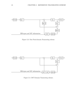
A Fast Pixel Domain (FPD) [8] Transrating scheme is shown in Fig.2.3. It comes
to improve the CPD scheme. It reuses the MB type’s decisions as well as initial
Motion Vectors (MVs), and thus greatly reduces the encoding complexity. It also
utilizes the linearity of motion compensation and of DCT/IDCT to reduce the mul-
tiple blocks in the CPD scheme. It is important to mention that while CPD Memory
buffers are saving pixel domain predicted frames, FPD Memory buffer (MEM) con-
tent is reconstructed requantization error that has to be added to DCT dequantized
coefficients to avoid error drift.
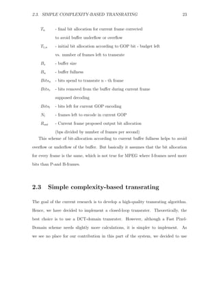
FPD transrating needs to return to the pixel domain in order to apply motion com-
pensation on the requantization error. However, Motion compensated DCT blocks
can be calculated directly in the DCT Domain as the sum of up to four source DCT
blocks multiplied by appropriate DCT-domain shift-matrices [10]. Hence, a DCT
Domain (DD) Transrating scheme can be built as shown in Fig.2.4. It was shown in
[10] that the number of calculations needed in this case is lower than when applying
IDCT, motion compensation and then DCT. However, existing DCT/IDCT acceler-
ators make this solution attractive only for strong hardware development companies.](https://image.slidesharecdn.com/13642942-120715025949-phpapp01/85/Michael_Lavrentiev_Trans-trating-PDF-25-320.jpg)
![2.2. DYNAMIC RATE-CONTROL FOR TRANSRATING 19
2.2 Dynamic Rate-Control for Transrating
There are several methods for dynamic bit-rate control. All of them are based on
tracking the available bit-rate status and updating the quantization scale accordingly.
Rate control can be separated into two steps: Picture layer bit-allocation, which
determines the target bit-budget for each picture, and macroblock layer rate-control
that determines the quantization parameters for coding the macroblocks. Sometimes
picture level bit-budget allocation can be downscaled to slice level. The simplest
frame-level scheme [21] proposes to divide the new bit-budget among frames using
the same ratio that they get in the input stream:
Rout Tout
= = const (2.1)
Rin Bin
where:
Rout - desired output average bit-rate
Rin - input sequence average bit-rate
Bin - bits spent on current frame in input stream
Tout - target bit allocation for the transrated frame
This approach is straight-forward. It does not provide any problem with virtual
buffer fullness - the buffer size can be simply decreased by the same ratio the stream
rate goes down. But the output stream quality is not the best possible one because
quality reduction of the I-pictures and the P-pictures impacts total video quality more
than it does for the B-frames. So another approach [21] proposes to provide the same
reduction ratio for all frames as in Eq.( 2.1), but to use for I-frames the square root
of the ratio of output/input bit-rates; for P-frames - the above ratio itself, and for](https://image.slidesharecdn.com/13642942-120715025949-phpapp01/85/Michael_Lavrentiev_Trans-trating-PDF-27-320.jpg)
![20 CHAPTER 2. REFERENCE TRANSRATING SCHEME
B-frames the ratio that will adjust the GOP bit-budget to the desired rate:
Rout
Rf
(1 + NP + NB ) − Sout,I (i − 1) − Sout,B (i − 1) − NP
S
nP out,P
(i − 1)
TB = (2.2)
Rin
Rf
(1 + NP + NB ) − Sin,I (i − 1) − Sin,B (i − 1) − NP
S (i − 1)
nP in,P
where:
TB - bit-budget for current B-frame
NP , NB - number of P- ,B- frames in GOP
nP - number of already transrated P- frames in GOP
Rout , Rin - designated output or input bit rates
Rf - frame-rate
Sout/in,I/P/B (i − 1) - bit-budget allocated by already transrated
I-,P-,B-frames in input/output bitstreams
Picture layer bit-budget allocation in a GOP based on picture complexity is pro-
posed in [22]. Picture complexity is defined as the product of the average quantizer
step-size and the number of bits generated, divided by some empirical constant. To
estimate the current picture complexity, the ratio of output/input complexities in
the previously transrated frame is multiplied by input complexity of the currently
transrated frame:
SP QP SB QB
XI = SI QI , XP = , XB = (2.3)
KP KB
where
S I , SP , SB - number of bits generated by encoding
of I-,P- and B-frames, respectively
QI , QP , QB - average quantization step sizes used in encoding
K P , KB - universal constants (1.0 and 1.4)
The allocation of the current frame-budget in the GOP is proportional to its](https://image.slidesharecdn.com/13642942-120715025949-phpapp01/85/Michael_Lavrentiev_Trans-trating-PDF-28-320.jpg)
![2.2. DYNAMIC RATE-CONTROL FOR TRANSRATING 21
complexity, for example, for I-frames:
Xout,I
Xin,I
Xin,I
TI = Np
TGOP (2.4)
Xout,I Xout,P NB X
out,B
Xin,I
Xin,I + Xin,P
Xin,P (i) + Xin,B
Xin,B (i)
i=1 i=1
where
TI - bit-budget for I-frame.
TGOP - bit-budget for the whole GOP
Xout,[I/P/B] - average output complexity of transrated I/P/B frames
in previous GOP
Xin,[I/P/B] - average input complexity of transrated I/P/B frames
in previous GOP
Xin,[I/P/B] - input complexity of frames in current GOP
Bit-budgets for P- and B-frames are calculated in a similar way. For open-loop
schemes, it was proposed to add a weighting factor to the ratio of averaged in-
put/output complexities which is the square root of relative picture depth [23]. There
is no clear explanation about how that depth is defined. Another simplification to
Eq.( 2.4) is proposed in [24],[25]:
Xout,n−type
Xin,n−type
Xin,n
Tn = Xout,P Xout,B
TGOP (2.5)
Xout,I + NP KP
+ NB KB
where](https://image.slidesharecdn.com/13642942-120715025949-phpapp01/85/Michael_Lavrentiev_Trans-trating-PDF-29-320.jpg)
![22 CHAPTER 2. REFERENCE TRANSRATING SCHEME
Tn - bit-budget for n-th frame
TGOP - bit-budget for the whole GOP
Xout,[I/P/B] - average output complexity of transrated I/P/B frames
that are transrated already
Xin,[I/P/B] - average input complexity of transrated I/P/B frames
that are transrated already
Xin,n - input complexity of the current frame
N[P/B] - Number of P/B frames in current GOP
In case the transrating mechanism does not provide the exact number of bits for
the particular frame, the same work [25] proposes to modify the bit-rate control to
allocate the bits left in the current GOP between the frames left according to there
complexities similar to Eq.( 2.4). The main drawback of complexity-based methods
is the lack of virtual buffer status verification. To take care of it, a buffer-controlled
scheme is proposed in [26]:
⎧
⎪
⎪ max{Rout , 0.9Bs − Bn } if
⎪
⎪ Bn + T1,n > 0.9Bs
⎨
Tn = Bitsr − Bn + 0.1Bs if Bn + T1,n − Bitsr < 0.1Bs
⎪
⎪
⎪
⎪
⎩ T1,n otherwise (2.6)
Bn +2(Bs −Bn )
T1,n = 2Bn +(Bs −Bn )
max{Rout , 0.95 Bitsl + 0.05Bn−1 }
Nl
Bn = Bn−1 + Bitsn−1 − Bitsr
where](https://image.slidesharecdn.com/13642942-120715025949-phpapp01/85/Michael_Lavrentiev_Trans-trating-PDF-30-320.jpg)
![24 CHAPTER 2. REFERENCE TRANSRATING SCHEME
the FPD transrating architecture. GOP-level rate-control takes a lot of attention in
recent works, but providing the best quality with matching rate and virtual buffer
constraints at the same time is still an open issue. We choose therefore a simple
solution that doesn’t provide problems with virtual buffer fullness: the bit-budget
reduction is according to Eq. (2.1). The last thing we have to decide on is how to
implement the frame-level bit-rate control. This is what we are going to present in
this section. It is possible to see that Eq.(2.4),(2.5) provide a bit budget to every
frame of the same type according to its input complexity Xin,n . To further simplify
the problem, we assume that complexity reduction is the same for all kinds of MBs
in the same frame. In this case the ratio of input complexities must remain the same,
and we can estimate the output bit-rate of MBs left to encode by bit-allocation of
the last encoded MB, and update the quantization step-size accordingly:
⎧
⎪ ind
⎪ q2,n + 1 if Bout > Bout
ˆ N
⎪
⎪ Xk
⎨
ind ˆ n+1
q2,n+1 = q ind − 1 if Bout < Bout
ˆ , Bout = (2.7)
⎪ 2,n
⎪ q tab[q2,n ] ·
ind
Bn
⎪
⎪
⎩ q ind ˆ
if Bout = Bout
2,n
where
Bn - bit allocation of the last transrated n-th MB
ˆ
Bout - estimated bit number needed to encode MBs left
Bout - bits left to encode the rest of the frame
ind
q2,n - index of last quantization step-size used
q tab[ ] - quantization step-size table used to get
appropriate quantization step-size value](https://image.slidesharecdn.com/13642942-120715025949-phpapp01/85/Michael_Lavrentiev_Trans-trating-PDF-32-320.jpg)
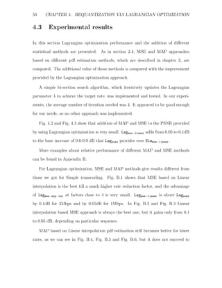
![2.4. EXPERIMENTAL RESULTS 27
container foreman
42 40.5
40
41
39.5
39
40
38.5
PSNR [dB]
PSNR [dB]
39 38
Sim 37.5
Enc
38 Sim
Re
37 Enc
Re
37 36.5
36
36
35.5
1 1.2 1.4 1.6 1.8 2 2.2 2.4 2.6 2.8 3 1 1.2 1.4 1.6 1.8 2 2.2 2.4 2.6 2.8 3
rate [bps] 6
x 10 rate [bps] x 10
6
hallmonitor tennis
40.5
35
40
39.5 34
39
PSNR [dB]
33
PSNR [dB]
38.5
38
32
Sim
37.5 Sim Enc
Enc Re
Re 31
37
36.5
30
36
1 1.2 1.4 1.6 1.8 2 2.2 2.4 2.6 2.8 3 1 1.2 1.4 1.6 1.8 2 2.2 2.4 2.6 2.8 3
rate [bps] x 10
6 rate [bps] 6
x 10
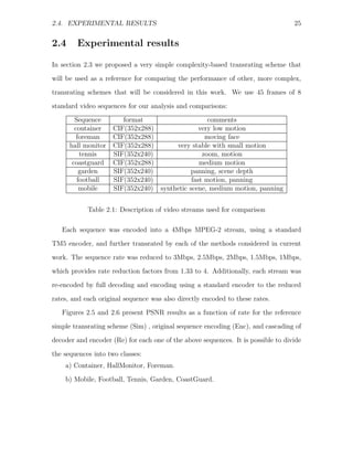
Figure 2.5: Simple transrating compared with TM5 encoded and Re-encoded.](https://image.slidesharecdn.com/13642942-120715025949-phpapp01/85/Michael_Lavrentiev_Trans-trating-PDF-35-320.jpg)
![28 CHAPTER 2. REFERENCE TRANSRATING SCHEME
coastguard garden
37
31
36
30
35 29
PSNR [dB]
PSNR [dB]
28
34
Sim
Enc
Re 27 Sim
Enc
33 Re
26
32
25
31
1 1.2 1.4 1.6 1.8 2 2.2 2.4 2.6 2.8 3 1 1.2 1.4 1.6 1.8 2 2.2 2.4 2.6 2.8 3
rate [bps] x 10
6 rate [bps] 6
x 10
football mobile
33
29
32 28
31 27
PSNR [dB]
PSNR [dB]
26
30
Sim
Enc 25
29 Re Sim
Enc
Re
24
28
23
27
1 1.2 1.4 1.6 1.8 2 2.2 2.4 2.6 2.8 3 1 1.2 1.4 1.6 1.8 2 2.2 2.4 2.6 2.8 3
rate [bps] x 10
6 rate [bps] 6
x 10
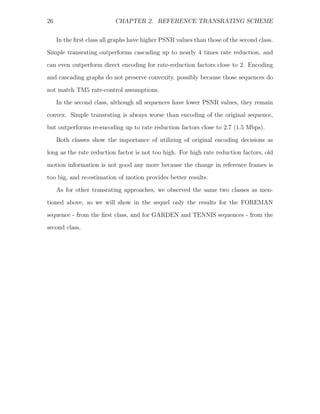
Figure 2.6: Simple transrating compared with TM5 encoded and Re-encoded.](https://image.slidesharecdn.com/13642942-120715025949-phpapp01/85/Michael_Lavrentiev_Trans-trating-PDF-36-320.jpg)
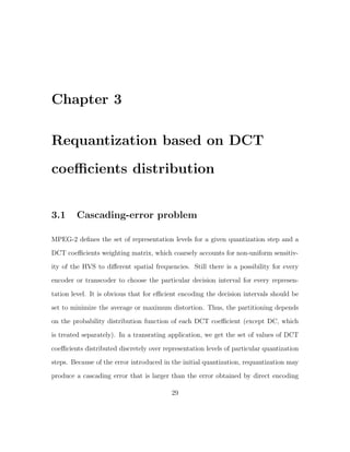
![30 CHAPTER 3. REQUANTIZATION BASED ON DCT COEFF. DISTR.
(a) (b)
Figure 3.1: (a) no cascading error introduced (b) cascading error due to requantization
is greater than error of direct quantization.
with the same quantization step, as described in [4] and shown in Fig. 3.1.
A method for reducing the cascading error is proposed in [29]. It is based on the
assumption that all decision regions are uniformly distributed and symmetric. Two
terms are proposed. The first is termed the critical requantization ratio, between
initial and final quantization steps, that may result in the biggest possible cascading
error, like Q2 /Q1 = 2 in the example below. The second is termed the optimal ratio
as it is a ratio that doesn’t cause cascading errors at all, like Q2 /Q1 = 3 in the
following example. The idea is, of course, to avoid critical ratios and, furthermore,
if the ratio proposed by the bit-rate control mechanism is near the optimal one, the
proposed quantization step size is changed to yield an optimal ratio. Fig. 3.2 gives
examples of optimal and critical requantization ratios, assuming a uniform midstep
quantizer with no dead zone (also known as midtread quantizer - see Fig. 3.5(a)).
For the critical ratio, Q2 = 2Q1 , where Q1 , Q2 denote the original and transrating](https://image.slidesharecdn.com/13642942-120715025949-phpapp01/85/Michael_Lavrentiev_Trans-trating-PDF-38-320.jpg)
![3.1. CASCADING-ERROR PROBLEM 31
Interval , contributing
to cascading error
decision Q1 Q1/2 reconstruction
levels levels
Q2=2Q1
(a)
decision Q1 reconstruction
levels levels
Q2=3Q1
(b)
Figure 3.2: (a) range supporting cascading error is maximal (b) no cascading error
introduced.
quantization step-sizes, respectively, every decision level defined by Q2 will always be
equal to one of the representation levels defined by Q1 . Thus, the range of values that
will be requantized to a different value than that of direct quantization will be equal
to Q1 /2 for every representation level produced by Q2 , as shown in Fig. 3.2(a). For
an optimal ratio, Q2 = 3Q1 , every decision level defined by Q2 will always be equal
to one of decision levels defined by Q1 and no cascading error will be introduced,
as seen in Fig. 3.2(b). One of the first approaches that take the distribution of
transform coefficients into account is proposed in [6]. A parametric rate-quantization
model, based on traditional rate-distortion theory, is applied to MPEG encoders.
Given the bit-rate budget for a picture, this model calculates a baseline quantization](https://image.slidesharecdn.com/13642942-120715025949-phpapp01/85/Michael_Lavrentiev_Trans-trating-PDF-39-320.jpg)
![32 CHAPTER 3. REQUANTIZATION BASED ON DCT COEFF. DISTR.
scale factor. For a rate-distortion analysis, the coefficients are assumed in [6] to be
Gaussian random variables, and the distortion to be proportional to the square of the
quantization step.
The variance of every transform coefficient in intra-frames was estimated and so
the distortion and rate for every quantization step is calculated by:
N N
1 σ2
R = r1 + log2 i , D = d1 + di (3.1)
i=2
2 di i=2
where,
N - number of transform coefficients
2
σi - estimated variance of i-th coefficient
di - quantization distortion (proportional to Q2 )
i
d 1 , r1 - distortion and bit-rate of DC coefficient
R - bit-rate estimation
D - estimated distortion
MPEG-2 provides different encoding of DC coefficients in intra-blocks than for
the rest of DCT coefficients, so the bit-rate and distortion for DC have to be cal-
culated separately. Assuming that the distortion is proportional to the square of
the quantization step-size and of the appropriate factor from quantization matrix, [6]
uses eq.(3.1) to estimate the output bitrate. One step-size for the whole frame, which
provides the closest rate to the bitrate constraint, is chosen. In a similar way the
procedure is applied for non-intra-frames and is used for optimal quantization step
estimation at the picture-level.](https://image.slidesharecdn.com/13642942-120715025949-phpapp01/85/Michael_Lavrentiev_Trans-trating-PDF-40-320.jpg)
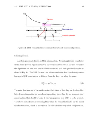
![3.2. MAP AND MSE REQUANTIZATION 33
r1
Figure 3.3: MAP requantization decision is taken based on probabities p1 and p2 .
3.2 MAP and MSE requantization
To address the problem of cascading error described in section 3.1, it is necessary to
take into account the probability distribution of input values. The idea of Maximum
A-Posteriori (MAP) requantization was introduced by Werner in [30]. Instead of
checking quantization ratios without questioning the optimality of the decision inter-
vals, as in section 3.1, the MAP approach minimizes the average cascading error by
an optimal mapping from a given set of initial encoding representation levels to the
defined requantization representation levels. The problem can be seen as changing the
decision intervals on requantization scale for each pair of initial and requantization
step sizes. The quantization step-size selection defines particular representation levels
for initial quantization and requantization. The MAP requantization method aims at
minimizing the probability of representing original input values by a representation
value different from the value that would be assigned to it by direct quantization.
Fig. 3.3 presents an initial pdf function p(x) and initial quantization and requanti-](https://image.slidesharecdn.com/13642942-120715025949-phpapp01/85/Michael_Lavrentiev_Trans-trating-PDF-41-320.jpg)
![34 CHAPTER 3. REQUANTIZATION BASED ON DCT COEFF. DISTR.
zation decision and representation levels. r1 is the representation level of decision
interval [d1 , d2). The initial quantization scale is defined by quantization step-size Q1
and the lower boundary of the decision interval d1 . The requantization scale (without
MAP) is defined by Q2 and the corresponding boundary D. This scale is denoted as
’reference’. The decision to be taken by MAP quantization is whether the values in
[d1 , d2 ) should be mapped to R1 or to R2 . For this purpose the probability that the
values that are mapped to R1 come from the interval [d1 , D) is compared with the
probability that they come from the interval [D, d2). If the first probability is bigger,
than interval will be mapped to R1 , otherwise to R2 .
The MAP decision rule minimizes the cost function that represents how much
MAP quantization is different from the direct encoding decisions:
E (y2,ref − y2 )2 |y1,ref (3.2)
Assuming that the transform coefficients pdf is Laplacian with parameter α:
α −α|x|
p(x) = e , (3.3)
2
√
2
where α is related to the standard deviation σ via σ = α
. It is claimed in [16] that
this is an appropriate pdf for DCT coefficients of Intra frames. The MAP rule in this
case becomes: ⎧
⎪
⎨ R1 , D−d1 >
q1
v1
2
y2 = Q2 (y1 = r1) =
⎪
⎩ R2 , D−d1 <
q1
v1
2
(3.4)
1 2
v1 = αQ1
ln 1+e−(αQ1 )
This mapping can be calculated offline with some assumptions on the initial pdf, or
estimated online from particular video stream statistics, as will be described in the](https://image.slidesharecdn.com/13642942-120715025949-phpapp01/85/Michael_Lavrentiev_Trans-trating-PDF-42-320.jpg)
![36 CHAPTER 3. REQUANTIZATION BASED ON DCT COEFF. DISTR.
Figure 3.5: (a) midstep quantizer with no dead zone (b) midrise quantizer.
One of the possible extensions of the above results is to analyze the distribution of
coefficients in a closed-loop transcoder before requantization and to use it for the
optimal definition of decision intervals /representation values.
3.3 Estimation of pdf parameters
MAP and MSE requantization, as any method based on the statistical distribution
of the initial DCT values, requires knowledge of the pdf, usually determined by its
parameters. In [31] a method for estimating the Laplacian parameter a of the DCT
coefficients (see eq. (3.3)) from the encoded coefficients distribution is proposed. It
can be estimated for each pdf of every DCT coefficient, in every block of each MB,
from the statistics of the current frame, or for each DCT coefficient in the entire
frame, while tracking its statistics over time. It is shown in [31] that for a uniform
midstep quantizer with no dead zone (Fig. 3.5(a)), the Laplacian parameter α could
be estimated by solving the following quadratic equation for z:
(A + B + C)z 2 + Bz − A = 0 (3.6)](https://image.slidesharecdn.com/13642942-120715025949-phpapp01/85/Michael_Lavrentiev_Trans-trating-PDF-44-320.jpg)
![3.3. ESTIMATION OF PDF PARAMETERS 37
where,
N
A= (yl − 2 )
q
,with N - number of coeff.,
l=1,yl =0
N0 q
B= 2
,with N0 - number of zero coeff.,
C = (N − N0 )q,
q
Then, for from the relation z = e−(ˆ 2 ) , the estimated parameter is
α
2
α = − ln z
ˆ (3.7)
q
For a uniform midrise quantizer, shown in Fig. 3.5(b), the equation becomes:
(A + B)z − A = 0 (3.8)
where,
N
A= (yl − 2 ),
q
l=1
Nq
B= 2
.
And the estimation for α is again α = − 2 ln z. These results were obtained in [31]
ˆ q
by using Maximum-Likelihood (ML) estimation.
Another work [32] proposes a method for estimating the Laplacian parameter α
from the variance of the quantized coefficients:
∞
eαq/2 + e−αq/2
vq = (nq)2 pn = q 2 , (3.9)
n=−∞
(eαq/2 − e−αq/2 )2
where,
nq+ q
2
pn = p(x)dx (3.10)
q
nq− 2
is the probability of the original coefficient value to fall into n-th decision interval.](https://image.slidesharecdn.com/13642942-120715025949-phpapp01/85/Michael_Lavrentiev_Trans-trating-PDF-45-320.jpg)
![38 CHAPTER 3. REQUANTIZATION BASED ON DCT COEFF. DISTR.
The Laplacian parameter is estimated as follows: From eq.( 3.9):
αq αq q2 + q 4 + 16vq
2
e /2 + e− /2 = =u (3.11)
2vq
hence,
√
αq u+ u2 − 4
e /2 = = t, (3.12)
2
resulting in,
2
α=
ˆ log t (3.13)
q
It predicts the quantization error, for the ideal case of infinite number of representa-
tion levels, to be:
q/2 nq+q/2
∞
2 αq
e2 = α x2 e−αx dx + α (x − nq)2 e−αx dx = (1 − αq/2 ) (3.14)
q
n=1
α 2 e − e−αq/2
0 nq−q/2
The estimation of α from (3.9) is not optimal in any sense, and the assumption of
an infinite number of possible quantization levels is not true for real implementations.
Still it provides a simple way for estimating α that typically supplies a good result.
Yet another method for estimating α is proposed by [33]. It is based on the empirical
number of zero valued coefficients and +q and -q valued coefficients. It is worse than
the previous method because it does not use all the statistics available for estimation,
but at this price it is less expensive computationally.](https://image.slidesharecdn.com/13642942-120715025949-phpapp01/85/Michael_Lavrentiev_Trans-trating-PDF-46-320.jpg)
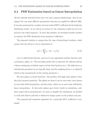
![42 CHAPTER 3. REQUANTIZATION BASED ON DCT COEFF. DISTR.
garden
31
30
29
PSNR [dB]
28
Simnone
Simmse−linear
27
Sim
mse−exp−ML
Sim
mse−exp−var
26
25
1 1.2 1.4 1.6 1.8 2 2.2 2.4 2.6 2.8 3
rate [bps] x 10
6
garden
24.55
24.5
24.45
24.4
PSNR [dB]
24.35 Sim
none
Simmse−linear
Simmse−exp−ML
24.3 Simmse−exp−var
24.25
24.2
9.4 9.5 9.6 9.7 9.8 9.9 10 10.1 10.2
rate [bps] x 10
5
Figure 3.6: MSE simple transcoding, GARDEN sequence.](https://image.slidesharecdn.com/13642942-120715025949-phpapp01/85/Michael_Lavrentiev_Trans-trating-PDF-50-320.jpg)
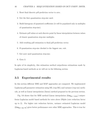
![3.5. EXPERIMENTAL RESULTS 43
garden
31
30
29
PSNR [dB]
28
27
Sim
none
Sim
map−linear
26 Simmap−exp−ML
Sim
map−exp−var
25
1 1.2 1.4 1.6 1.8 2 2.2 2.4 2.6 2.8 3
rate [bps] x 10
6
garden
27.5
27
26.5
PSNR [dB]
26
25.5 Simnone
Simmap−linear
Simmap−exp−ML
25 Simmap−exp−var
24.5
1 1.1 1.2 1.3 1.4 1.5 1.6 1.7
rate [bps] x 10
6
Figure 3.7: MAP simple transcoding, GARDEN sequence.](https://image.slidesharecdn.com/13642942-120715025949-phpapp01/85/Michael_Lavrentiev_Trans-trating-PDF-51-320.jpg)
![44 CHAPTER 3. REQUANTIZATION BASED ON DCT COEFF. DISTR.
garden
31.5
31
30.5
PSNR [dB]
30 Simnone
Sim
map−linear
Simmse−linear
Sim
map−exp−ML
29.5
29
28.5
2 2.1 2.2 2.3 2.4 2.5 2.6 2.7 2.8 2.9 3
rate [bps] 6
x 10
garden
27.5
27
26.5
PSNR [dB]
26 Simnone
Simmap−linear
Simmse−linear
Simmap−exp−ML
25.5
25
24.5
1 1.1 1.2 1.3 1.4 1.5 1.6 1.7
rate [bps] 6
x 10
Figure 3.8: compare MSE and MAP for simple transcoding, GARDEN sequence.](https://image.slidesharecdn.com/13642942-120715025949-phpapp01/85/Michael_Lavrentiev_Trans-trating-PDF-52-320.jpg)
![Chapter 4
Requantization via Lagrangian
optimization
MPEG-2 encoding provides output bit-rate control by changing the quantization step
size. The change in quantization step-size enables to achieve bit-rate reduction at
the cost of perceptual video quality. There are many questions that arise during
transrating, the most important of which are these:
1. How to achieve the desired bit-rate after transrating?
2. How to provide the best perceptual quality for the same rate?
In this chapter we review and examine optimal requantization via Lagrangian opti-
mization. Section 4.1 describes the standard MPEG-2 encoding procedure. Section
4.2 presents the Lagrangian optimization method proposed in [4, 5, 9, 10] to get opti-
mal requantization step-sizes for transrating. Experimental results and their analysis
are provided in section 4.3.
45](https://image.slidesharecdn.com/13642942-120715025949-phpapp01/85/Michael_Lavrentiev_Trans-trating-PDF-53-320.jpg)
![46 CHAPTER 4. REQUANTIZATION VIA LAGRANGIAN OPTIMIZATION
4.1 MPEG-2 AC coefficients encoding procedure
Following the application of the DCT to each of 4 luminance 8×8 blocks and to 2 up
to 8 chrominance blocks (depending on video format), which form a MB, the DCT
coefficients, except for the DC coefficient, are quantized. For each MB, a value from
one of two possible tables, each having 32 quantization step-size values, is selected
(a different table can be chosen for each frame). The actual quantization step-size
used for each coefficient is the product of the selected step-size from the table and
a value defined by a suitable quantization matrix that depends on the MB type.
The 63 quantized AC coefficients are concatenated in an order defined by one of two
possible zig-zag scans. The resulting 6 to 12 vectors, of 63 quantized coefficients each,
constituting a MB, are entropy coded by a variable-length-coding (VLC) table. Each
coefficient vector is divided into several parts, with each part consisting of a run of
consecutive zeros followed by a non-zero level value, defining a run-level pair. In case
of adjacent non-zero level values, the run length is defined to be zero. The MPEG-2
standard defines for every run-level pair a variable-length codeword. There are two
VLC tables that can be used. It is possible to use the same table for all types of MBs,
or to use a different one for Intra MBs [34].
4.2 Lagrangian optimization
The requantization problem can be formulated as an optimization problem of de-
termining a set of quantization step-sizes that minimize the total distortion in each
frame, under a given bit-rate constraint:
min D, under the constraint R ≤ RT (4.1)
{qk }](https://image.slidesharecdn.com/13642942-120715025949-phpapp01/85/Michael_Lavrentiev_Trans-trating-PDF-54-320.jpg)
![4.2. LAGRANGIAN OPTIMIZATION 47
with ,
N N
D= dk (qk ), R = rk (qk ), (4.2)
k=1 k=1
where,
N - number of MBs in the frame;
qk - quantization step-size for the k-th MB;
dk - distortion caused to the k-th MB;
rk - number of bits produced by the k-th requantized MB.
An analysis for the conventional MSE distortion metric is presented in [5]. The
problem can be converted into an unconstrained one by merging rate and distortion
through a Lagrange multiplier λ ≥ 0 into the cost function:
Jtotal = D + λR (4.3)
λ defines the relative importance of rate against distortion in the optimization pro-
cedure.
This constrains the set of possible solutions to a lower boundary of Convex Hull of
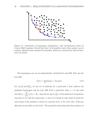
all possible solutions. Fig.4.1 shows the constraints of the Lagrangian solution. Points
show achievable rate-distortion states. The dotted blue line shows the boundary of
the Convex Hull of all possible solutions. Only states on the Convex Hull boundary
(blue points on blue dotted line) can be found by Lagrangian optimization. Red states
(connected by solid red line), which are optimal for particular rates, can’t be reached
using Lagrangian optimization. Lagrangian multiplier defines the rotation of the rate-
distortion axes before minimization. Under all possible rotations red state will never
be the minimum over all possible states. It reduces a bit from the optimality of the
solution, but assuming the set of all solutions is dense it should be good enough.](https://image.slidesharecdn.com/13642942-120715025949-phpapp01/85/Michael_Lavrentiev_Trans-trating-PDF-55-320.jpg)
![4.2. LAGRANGIAN OPTIMIZATION 49
[5] is:
⎧
⎪
⎪ [Ck (qk ) − Ck (qk )]2
⎪
⎪
ni ni
(intra)
1
L−1 63 ⎨
dk (qk ) = 2 [C ni (q ) − Ck (qk ) + Xk ]2
ni ni
(forward,backward) (4.5)
L ⎪ k k
⎪
n=0 i=0 ⎪
⎪
⎩ [C ni (qk ) − C ni (q ) + Xk +Ykni ]2
ni
(interpolated)
k k k 2
where,
ni
Ck (qk ) - i-th inverse quantized DCT coeff. of block n in MB k
ni ni
Ck (qk ) - same as Ck (qk ), but after requantization
Xk , Ykni
ni
- error drift from reference pictures (forward and/or backward)
L, n - number of blocks in MB and block index
k - index of MB
i - DCT coeff. index (64 DCT coeff in every block)
It is shown in [5], by simulations, that by using the same set of coding decisions
as produced by the initial encoder, optimal requantization can achieve higher PSNR
than that achieved by direct encoding of the original video sequence to the final lower
bit-rate by the usual encoder. This is possible because common encoders do not
perform this kind of optimization, for finding the best possible quantization steps, to
avoid an increase in the encoding complexity.
Lagrangian optimization is a general and very powerful method. It can also be
applied as in [35] to obtain the optimal discarding of DCT coefficients in I-frames. In
[17] it is applied to the discarding of high-frequency DCT coefficients only.](https://image.slidesharecdn.com/13642942-120715025949-phpapp01/85/Michael_Lavrentiev_Trans-trating-PDF-57-320.jpg)

![52 CHAPTER 4. REQUANTIZATION VIA LAGRANGIAN OPTIMIZATION
foreman
41
40
39
PSNR [dB]
38
Simmse−linear
Lagnone
Lagmse−linear
Lag
mse−var
37
36
1 1.2 1.4 1.6 1.8 2 2.2 2.4 2.6 2.8 3
rate [bps] x 10
6
football
33
32
31
PSNR [dB]
30
Sim
mse−linear
Lagnone
Lagmse−linear
29 Lag
mse−var
28
27
1 1.2 1.4 1.6 1.8 2 2.2 2.4 2.6 2.8 3
rate [bps] x 10
6
Figure 4.2: Comparison of Lagrangian vs. Simple transcoding for different sequences.](https://image.slidesharecdn.com/13642942-120715025949-phpapp01/85/Michael_Lavrentiev_Trans-trating-PDF-60-320.jpg)
![4.3. EXPERIMENTAL RESULTS 53
garden
32
31
30
29
PSNR [dB]
28
Simmse−linear
27 Lagnone
Lag
mse−linear
Lag
mse−var
26
25
1 1.2 1.4 1.6 1.8 2 2.2 2.4 2.6 2.8 3
rate [bps] x 10
6
tennis
36
35
34
PSNR [dB]
33
32 Sim
mse−linear
Lag
none
Lag
mse−linear
31 Lagmse−var
30
1 1.2 1.4 1.6 1.8 2 2.2 2.4 2.6 2.8 3
rate [bps] x 10
6
Figure 4.3: Comparison of Lagrangian vs. Simple transcoding for different sequences.](https://image.slidesharecdn.com/13642942-120715025949-phpapp01/85/Michael_Lavrentiev_Trans-trating-PDF-61-320.jpg)
![Chapter 5
Extended Lagrangian optimization
In this chapter we propose a novel extension of the Lagrangian optimization method
by applying modifications to the quantized DCT indices. The proposed method
outperforms (in terms of PSNR) all currently known requantization-based transrating
approaches. To reduce the algorithm’s complexity, we provide a low complexity trellis-
based optimization scheme, and discuss other complexity reduction means as well.
In section 5.1 we introduce the quantized DCT indices modification method and
define an extended Lagrangian minimization problem. Section 5.2 presents an effec-
tive solution based on a modification of the Viterbi trellis-search algorithm. Com-
plexity considerations and means for its reduction are discussed in section 5.3. Ex-
perimental results are presented and discussed in section 5.4.
5.1 Quantized DCT indices modification
The idea of modifying the levels of quantized DCT coefficients, before applying VLC,
for bit-rate reduction was proposed in [35, 17]. However, [35] discusses only methods
54](https://image.slidesharecdn.com/13642942-120715025949-phpapp01/85/Michael_Lavrentiev_Trans-trating-PDF-62-320.jpg)
![5.1. QUANTIZED DCT INDICES MODIFICATION 55
for excluding AC coefficients in I-frames, and [17] considers only discarding several
last non-zero coefficients in the zig-zag scan. We propose to extend the Lagrangian
optimization presented in the previous section to include the possible modification
of the values of all quantized DCT coefficients in an efficient way. The suggested
optimization procedure aims at choosing quantized AC coefficient vectors values, as
well as optimal quantization step sizes, that will provide a bit-rate that is as close as
possible to the desired one with minimal distortion possible for the same rate.
Direct encoding of requantized coefficients using a given fixed run-level coding
table does not necessarily provide the minimum possible distortion for a given total
rate. It is possible to reduce the bit-rate needed for encoding by changing the values of
the quantized vectors before run-level coding. To preserve the best possible quality at
a given bit-rate, the selection algorithm uses a distortion penalty, caused by selecting
reconstructed values away from the optimal one. An improvement, compared to
selecting optimal quantization step sizes only, is expected due to the following reasons.
For a particular quantization step size, it is possible sometimes to reduce the distortion
if the cascaded quantization value can be changed to a value that provides a better
approximation to the optimal reconstructed value. It is also possible to reduce the
total bit-rate by breaking VLC pairs with long runs into several smaller ones that
give a smaller total bit-rate than that of the initial pair. Of course, it increases the
distortion most of the time. The goal is to reduce the bit-rate needed to encode some
of the coefficients so that the distortion in other coefficients can be reduced.
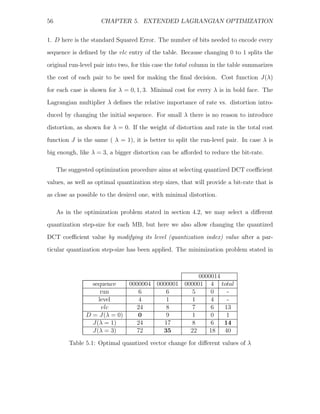
Table 5.1 gives an example of possible quantized run-level pair changes. Let
0000004 be the quantized run-level pair to be encoded by the MPEG-2 VLC table.
Suppose that we can choose if to encode it as is (i.e. without introducing any addi-
tional distortion D); to enter a 1 instead of the last 0, or to change the value 4 into](https://image.slidesharecdn.com/13642942-120715025949-phpapp01/85/Michael_Lavrentiev_Trans-trating-PDF-63-320.jpg)
![62 CHAPTER 5. EXTENDED LAGRANGIAN OPTIMIZATION
40 24
22
35
20
30
18
25 16
level 14
20
12
15
10
10 8
6
5
4
5 10 15 20 25 30
run
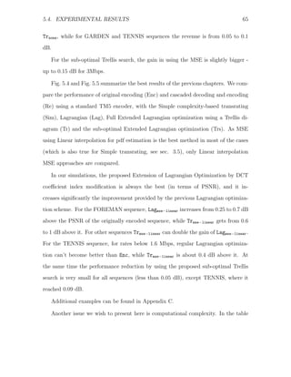
Figure 5.3: one of two possible MPEG-2 VLC tables.
As for quantization step-sizes, there were a number of works that propose to re-
strict the range of requantization step-sizes based on the initial MB quantization
step-size [27, 28, 23].The most recent [23] shows that for open-loop transcoding La-
grangian optimization [4] can be restricted to check even and odd multiples of the
initial quantization step-size for I and P-B frames, respectively. At those ratios many
quantized coefficients are zeroed out after rounding. The optimal multiples of the
initial quantization step-size are changing according to different quantizers used for I
and P,B-frames, as shown in Fig. 3.5. The results reported for the closed-loop scheme
were very close to those of full Lagrangian search. As for searching over different val-
ues of λ, applying a simple bi-section search, as in [5], requires on average about 3
iterations only.](https://image.slidesharecdn.com/13642942-120715025949-phpapp01/85/Michael_Lavrentiev_Trans-trating-PDF-70-320.jpg)
![5.4. EXPERIMENTAL RESULTS 67
foreman
41
40
39
PSNR [dB]
38
Trmse−linear
Trs
mse−linear
Lag
mse−linear
Simmse−linear
37
Enc
Re
36
1 1.2 1.4 1.6 1.8 2 2.2 2.4 2.6 2.8 3
rate [bps] x 10
6
garden
32
31
30
29
PSNR [dB]
28
Tr
mse−linear
Trsmse−linear
27
Lagmse−linear
Sim
mse−linear
26 Enc
Re
25
1 1.2 1.4 1.6 1.8 2 2.2 2.4 2.6 2.8 3
rate [bps] 6
x 10
Figure 5.4: Best MSE transrating for all methods for different sequences.](https://image.slidesharecdn.com/13642942-120715025949-phpapp01/85/Michael_Lavrentiev_Trans-trating-PDF-75-320.jpg)
![68 CHAPTER 5. EXTENDED LAGRANGIAN OPTIMIZATION
football
33
32
31
PSNR [dB]
Trmse−linear
30
Trsmse−linear
Lag
mse−linear
Simmse−linear
29 Enc
Re
28
27
1 1.2 1.4 1.6 1.8 2 2.2 2.4 2.6 2.8 3
rate [bps] x 10
6
tennis
36
35
34
PSNR [dB]
33
Trmse−linear
32 Trsmse−linear
Lagmse−linear
Sim
mse−linear
31 Enc
Re
30
1 1.2 1.4 1.6 1.8 2 2.2 2.4 2.6 2.8 3
rate [bps] x 10
6
Figure 5.5: Best MSE transrating for all methods for different sequences.](https://image.slidesharecdn.com/13642942-120715025949-phpapp01/85/Michael_Lavrentiev_Trans-trating-PDF-76-320.jpg)
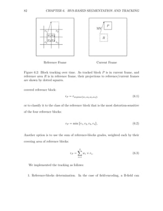
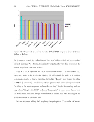
![70 CHAPTER 6. HVS-BASED SEGMENTATION AND TRACKING
the decoded video seems to be a better solution. The following section aims at video
segmentation for transrating applications. Transrating input is compressed-domain
data, and so is the output. More precisely, the current research deals with MPEG-
2 transrating, i.e. reducing the bitrate of already block-based DCT encoded video.
Section 6.2 describes the segmentation scheme we used in this work for transrating.
Results of the proposed scheme are shown in section 6.3.
6.1 Existing Compressed Domain
Segmentation Methods
Following [36], features used by compression domain segmentation schemes are:
1. DC value of DCT, which is the mean luminance value of the block, known as µ
in pixel-based methods.
2. Sum of squared AC coefficients, which corresponds to the variance in pixel
domain.
3. Sums of amplitudes of AC coefficients in the first row and first column of the
DCT coefficient matrix was proposed as a measure for vertical and horizontal
edge presence in a block by [37]. More complex DCT domain edge detection
method are proposed in [38].
4. Color: DC values of Y, Cb and Cr color component blocks can be used to form
a block’s color vector[39].
5. Motion Vectors (MV) presented in Inter-coded pictures and blocks.](https://image.slidesharecdn.com/13642942-120715025949-phpapp01/85/Michael_Lavrentiev_Trans-trating-PDF-78-320.jpg)
![6.1. EXISTING COMPRESSED DOMAIN SEGMENT. METHODS 71
6. MB bit-count information multiplied by quantization step size can provide in-
formation about coding complexity of the particular MB that shows how hard
it is to reduce the MB bit-count by increasing the quantization step-size.
7. MB coding type must be taken into account while making decisions about spe-
cific block classification.
Segmentation approaches can be divided into two main groups:
1. Local-properties-based methods. These methods assume that what is important
for a human observer looking on a particular region of a picture are the local
region properties themselves, with some minor correlation to the adjacent areas
features, like mean luminance.
2. Object-based methods. These methods presume that a human observer identi-
fies different objects in a video sequence, and what is important to him is the
better quality of the important video objects in the scene.
6.1.1 Methods based on local properties
These methods are based on extracting local features from compressed domain data,
like blockiness [40] or boundaries [38], which can be used to define the perceptual
importance of a particular image block. It is also important to remind here works
that aim to define perceptual quality based on the DCT domain information. Some
of those works still need the original picture for comparison [41], which is not the case
we have in transrating.
In [42] it is proposed to calculate perceptual activity of every block based on the
DCT coefficients weighted by a correlation matrix computed in a bigger neighboring](https://image.slidesharecdn.com/13642942-120715025949-phpapp01/85/Michael_Lavrentiev_Trans-trating-PDF-79-320.jpg)
![72 CHAPTER 6. HVS-BASED SEGMENTATION AND TRACKING
area centered at the same block. The ratio of a particular block and neighboring areas
DC values is supposed to take into account Weber’s law. This ratio is appropriately
combined with the sum of absolute values of weighted DCT AC coefficients to measure
the perceptual activity of that block.
Considering implementations for transrating, it turns out that there are not so
many works published that are based on local properties as there are about object-
oriented methods. The methods utilized are also much simpler.
In [43] a Hybrid Transrating method that switches between requantization, re-
sizing and frame skipping was proposed. The decision is made at frame level, so
the measures proposed were Motion Activity, which is the average magnitude of the
motion vectors of all the macroblocks in each frame, and Spatial Activity, which is de-
fined as the mean quantization step-size, or the actual number of bits used to encode
the frame if the first the mean quantization step-size exceeds its maximum value.
Another frame-based MPEG properties extraction that aims at transrating was
proposed in [44]. Quantization step-size is called Region Perceptibility and the num-
ber of zero DCT coefficients in the block is defined as Spatial Complexity. As Tem-
poral Similarity features, it is proposed to gather MB coding type, the direction of
MVs (forward, backward or bi-directional), prediction type (frame or field), and the
number of actual MVs used for a particular MB (from one up 4 in bi-directional
field predicted MB). The work deals mainly with MPEG-2 to MPEG-4 transrating
and does not target requantization, i.e. transrating problem. So the major aspect
analyzed was which properties can be re-used, and which has to be modified and how
to meet MPEG-4 standard specifications.
Some encoding techniques can be adapted to transrating. It is mentioned in [45]
that objectionable artifacts that occur when pictures are encoded at low bit rates](https://image.slidesharecdn.com/13642942-120715025949-phpapp01/85/Michael_Lavrentiev_Trans-trating-PDF-80-320.jpg)
![6.1. EXISTING COMPRESSED DOMAIN SEGMENT. METHODS 73
are: blockiness, blurriness, ringing and color bleeding. Blockiness is related to high
quantization of smooth regions, while ringing and color bleeding occur at edges on flat
background where high frequencies are poorly quantized. Blurriness is the result of
loss of spatial detail in moderate- and high-detailed regions. To avoid producing those
artifacts, the MBs are classified into either homogeneous or edge-including, based on
a comparison of MB block’s variances. Homogeneous MBs are further sorted into
several classes from flat to coarse-textured. At the same time edge-including MBs
are arranged into sub-classes as weak edge, normal edge, strong edge and structured
edge. A similar approach can be implemented for transrating, with a further bit-rate
allocation that is proportional to each class perceptual importance, as it is done in
encoding.
6.1.2 Object oriented Methods
There are many efforts to perform object segmentation of a video stream. Most of the
works were motivated by the MPEG-4 standard that enables Video Object Planes
(VOP) encoding. To prepare tools for MPEG-2 to MPEG-4 conversion, many authors
propose segmentation algorithms working in the compressed domain.
Several researches try to segment the video on the basis of MV information. MVs
can be accumulated over time to build dense motion information for every pixel in the
frame and to use it for pixel-domain segmentation. Such segmentation can maximize
the probability that all pixels in a particular segment share the same affine trans-
formation [46]. The pooling of MVs from multiple frames is also used for building a
more robust data set for clustering [47]. To withstand MV estimation errors, the data
set includes all MBs with MV close enough to currently estimated affine models, and
after that the data is re-clustered, and the affine models are updated. Segmentation](https://image.slidesharecdn.com/13642942-120715025949-phpapp01/85/Michael_Lavrentiev_Trans-trating-PDF-81-320.jpg)
![74 CHAPTER 6. HVS-BASED SEGMENTATION AND TRACKING
tracking needed in transrating is usually exploited in background freezing approaches
that can be used for fixed camera scenes. If an initial block-based segmentation is
known, the tracking can utilize MV information of encoded MPEG stream to detect
what new blocks are covered by projections of the initial object MBs [48]. The MBs
are divided into Active (predicted objects), Monitored (MBs that are close enough
to the objects) and Inactive. A set of rules define how some objects MBs can be
transferred either to Monitored or Inactive clusters, and how MBs from Active or
Monitored partitions can be transferred to an Active set.
DCT coefficients similarity can be defined and used for image segmentation in
many different ways. For example, it is possible to calculate the DCT of a block cen-
tered at every pixel in the picture, and by PCA to define the number of dominant re-
gions in the scene. By using appropriate filters it is possible to fit the DCT coefficients
to frequency characteristics of HVS, and so get perceptually adapted segmentation
after K-means clustering on what is called Situational DCT Descriptors[49].
The combination of DCT and MV information for moving objects extraction was
also tested in a number of works. Region Growing methods often use a spatial feature
vector that consists of mean block luminance, vertical edge, horizontal edge and
texture (see section 6.1 features 1,2 and 4). Following segmentation, the region is
set to be a moving region if more than a half of its MBs have non-zero MVs [50].
This approach is sensitive to MV estimation errors, so the possibility of false motion
has to be minimized by comparing coded motion residual with no motion residual,
which has to be calculated additionally by the proposed scheme. A somewhat more
complex classification of false motion blocks was proposed in [51]. It checks if blocks
adjacent to a particular block in the direction of its motion are also dynamic. A
possible combination is assigned using the ratio of probabilities of the realization](https://image.slidesharecdn.com/13642942-120715025949-phpapp01/85/Michael_Lavrentiev_Trans-trating-PDF-82-320.jpg)
![6.1. EXISTING COMPRESSED DOMAIN SEGMENT. METHODS 75
of this combination assuming ”real moving block” to that assuming ”false moving
block”.
Another way to segment Intra frames is to employ the Watershed method [52],
which is widely used in the pixel domain, to a simplified image consisting of the DC
values only or DC plus 2 AC coefficients picture [53]. The Watershed method is used
to produce closed smooth areas coverage of the initial image, based on a gradient
image. One of the method drawbacks is that it usually over-segments the image
due to local noise in the picture. To avoid over-segmentation, leveling that uses as
a marker the DC image and the DC+2AC image as reference is employed. Markers
mark some of the initial zones as areas of interest, and the segmentation is constructed
starting from these zones, so better segmentation can be achieved. The largest flat
zones in the resulting image are chosen as markers for a final watershed segmentation,
which is based on morphological gradient of the leveled image. To find the moving
regions, the MVs of neighboring Inter frames are summed for every MB, and the
Manhattan distance is calculated on resulting MVs to represent the displacement,
which is further uniformly quantized into eight levels. This information can be used
for final segmentation, or for global motion estimation of the scene.
A more complex spatiotemporal segmentation scheme is proposed in [54]. The ini-
tial segmentation is generated by Sequential Leader Clustering of vectors combined
from DC of all three image color components and AC energy information. Sequen-
tial Leader Clustering algorithm uses pre-defined threshold and distance measure to
decide if new point has to be added to the closest of the existing clusters, or, if the
distance is above the threshold, has to start a new cluster. After a number of clusters
is defined, adaptive K-mean clustering is applied to adjust the initial segmentation.
The small regions are merged with their neighbors using luminance and AC energy](https://image.slidesharecdn.com/13642942-120715025949-phpapp01/85/Michael_Lavrentiev_Trans-trating-PDF-83-320.jpg)
![76 CHAPTER 6. HVS-BASED SEGMENTATION AND TRACKING
distances. Entropy values of ac energy for every region is calculated, and modeled
as a Gaussian distribution with mean µ and standard deviation σ, over all regions
in the picture. Then, spatial similarity is calculated for every pair of adjacent blocks
based on assumption that entropy difference must be of zero mean and of variance
√
2σ. The temporal similarity is derived based on the Kolmogorov-Smirnov hypoth-
esis test of the distribution of the temporal gradient. Kolmogorov-Smirnov statistic
is defined as the maximum value of the absolute difference between two cumulative
distribution functions. Temporal gradient is calculated by applying a 3-D Sobel filter.
It is not described in the letter [54] on which data in compressed domain, if at all,
it was applied. Finally, two similarity measures, one for merging spatiotemporally
similar regions (a modification of similarity measure proposed in [55]), and one for
merging regions with high average temporal change within the region, are calculated.
After Region Adjacency Graph (RAG) merging based on those similarity values, the
regions are classified as foreground or background based on average temporal change
of regions.
Another approach for clustering is Maximum Entropy Fuzzy Clustering (MEFC)
in the compressed domain. The idea of fuzzy clustering is to iteratively calculate
the region centers and to update each image sample membership based on some dis-
tance measure. In MEFC the distance from a pixel to every cluster is defined by the
squared difference of the pixel value from each cluster center value that is weighted
by a membership function. The membership function derivation is based on the prin-
ciple of maximum entropy to yield a least biased clustering. It is possible to use
MEFC on DC coefficients, and further to refine the membership of blocks surround-
ing the current object to be either foreground or background based on a Maximum
A Posteriori (MAP) approach applied to those block’s AC coefficients [56]. For video](https://image.slidesharecdn.com/13642942-120715025949-phpapp01/85/Michael_Lavrentiev_Trans-trating-PDF-84-320.jpg)
![6.2. PROPOSED SCHEME 77
it was proposed to use MEFC for segmentation of MV data projections on I-frame
from two P-frames surrounding the I-frame. To achieve finer VO’s boundary seg-
mentation, MEFC is further applied to DC coefficients of I-frames [57]. To avoid
problems caused by non-perfect MV information, it is assumed to be of impulse noise
nature, and is filtered by Noise Adaptive Soft-switching Median (NASM) filter [58].
The filtered MVs are then clustered by the MEFC algorithm. Validated regions are
tracked using Kalman filtering, which update second order motion model. Segmented
regions projection according to that motion data is used to make robust temporal seg-
mentation, which tests motion homogeneity and overlapping area of the segmented
masks, such that a recursive merging and splitting process could be performed in the
temporal domain [59]. DC coefficients of three color components are then clustered
into an optimum number of homogeneous regions, also by applying MEFC. To com-
plete the classification of the small homogeneous regions that are usually produced by
the proposed algorithm, MAP processing to classify those regions into either moving
foreground or stationary background is proposed.
6.2 Proposed Scheme
In the current research, segmentation is used to provide different perceptual impor-
tance to different parts of the picture so as to match the MSE distortion in those
areas to perceptual criteria. The algorithm described below uses the information
available in the encoded stream, like AC coefficients and motion vectors, to perform
a local-based segmentation. Each block in the picture gets a relative weight that car-
ries information on the extent the rate can be reduced in the particular block during
transrating.](https://image.slidesharecdn.com/13642942-120715025949-phpapp01/85/Michael_Lavrentiev_Trans-trating-PDF-85-320.jpg)
![78 CHAPTER 6. HVS-BASED SEGMENTATION AND TRACKING
The proposed segmentation scheme uses a somewhat simpler approach than [45].
It consists of two main units:
1. Encoded data segmentation unit, which partitions the picture into segments
based on the coded AC coefficients.
2. Tracking unit, which utilizes motion information to track the segments varia-
tions over time.
The segmentation technique developed suits both open-loop and closed-loop transrat-
ing schemes. So, only the information available in the DCT domain and the motion
vectors are used. As follows from the original goal of this scheme, the segmentation is
done at a resolution of 8×8 blocks. It is possible to replace the proposed segmentation
scheme by another one, and still utilize the tracking scheme to improve results over
time.
6.2.1 AC-based segmentation
Following [45], we assume that the amount of information in smooth areas is small,
hence so is its bit-budget. However, even a small reduction in their bit-rate typically
results in a visible degradation in picture quality. On the other hand, textured regions
in the picture demand many bits, but their rate can usually be significantly reduced,
before a human observer will notice the difference. Boundaries (edges) are known
to be the most perceptually important part of the scene, but in terms of rate vs.
noticeable distortion, they fall, on average, between smooth areas and textures. Thus,
the proposed scheme classifies blocks as being either smooth, textured or boundary.
It is possible to define a textured block as block that is surrounded by other boundary](https://image.slidesharecdn.com/13642942-120715025949-phpapp01/85/Michael_Lavrentiev_Trans-trating-PDF-86-320.jpg)
![6.2. PROPOSED SCHEME 79
blocks from almost all directions. It can either include boundary by itself, or not.
The segmentation algorithm thus consists of the following steps:
1. Block activity evaluation. The sum of absolute values of AC coefficients can be
a good measure for edge presence in a particular block [36]. DC and two first
AC coefficients are omitted, as not to take into account slow luminance changes
over flat areas.
2. Binarization. The block activity picture is converted into a binary picture
that classifies each block as either a high-activity block or low-activity block.
Binarization is done using adaptive thresholding. The Otsu method [60] uses
an interclass variance criterion for bilevel thresholding. It is simple and usually
gives very good results. This technique yields a threshold resulting in minimal
intra-class variance and maximal inter-class variance.
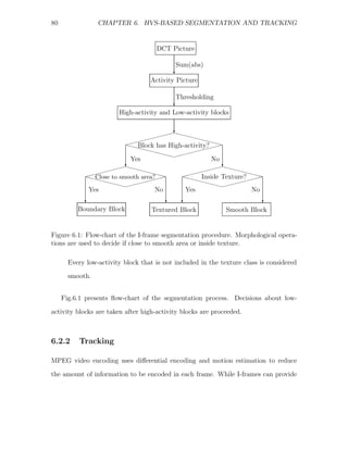
3. Texture detection. Morphological operations are used to remove from the set of
high-activity blocks the blocks that are close to relatively big low-activity areas.
The size and the form of these areas are defined via a particular selection of
structuring element. During these operations the edge between textured and flat
areas is removed, as well as small isolated blocks and thin boundaries between
smooth areas. Other operators are used to fill in small holes in the remaining
set of high-activity blocks to form textured areas.
4. Forming segmented picture. At this point, textured regions are already formed.
All the blocks that pass the threshold but were not included into the texture
class are classified as boundaries. It includes isolated active blocks in low-
activity areas, and boundaries between textured and smooth regions as well.](https://image.slidesharecdn.com/13642942-120715025949-phpapp01/85/Michael_Lavrentiev_Trans-trating-PDF-87-320.jpg)
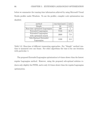
![7.1. SUMMARY AND CONCLUSIONS 93
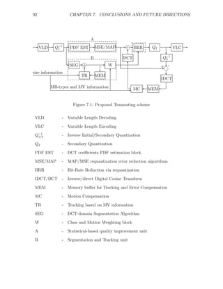
The proposed system is an extension of Fast Pixel Domain transcoder (see Fig.2.3).
Dashed boxes shows the functional blocks we contributed to.
The first and the most important part of this work is the development and evalua-
tion of different requantization algorithms. This thesis focuses on frame-level requan-
tization. In chapter 2 a fast complexity-based transrating algorithm is presented. For
this and all the following algorithms any GOP-level rate controlling scheme can be
applied.
Chapter 4 introduces Lagrangian optimization for quantization step-size selection
developed in [5]. This algorithm has provided the best PSNR for given bit-rate
constraints over all previously developed transrating algorithms.
We propose in this work to extend the Lagrangian optimization procedure by
allowing the modification of quantized DCT indices, including setting their val-
ues to zero, in addition to quantization step-size selection. Quantized DCT index-
modification and quantization step-size selection are optimally done using a low
complexity trellis-based procedure. The proposed requantization algorithm provides
higher PSNR values than the original Lagrangian-based optimization method that
only handles the selection of quantization steps, and still, practically, does not exceed
considerably its complexity.
The main problem of transrating is that the input video is already degraded by
lossy compression. In chapter 3 DCT coefficient PDF-based methods for requanti-
zation error minimization are discussed (see dashed box A, Fig.7.1), and the MSE
and MAP estimation methods are compared. It is commonly assumed that Lapla-
cian distribution is a good model for DCT coefficients distribution, and a number of
methods to estimate Laplacian distribution parameter were proposed in the literature.
However, we found that those methods do not provide good results, and developed](https://image.slidesharecdn.com/13642942-120715025949-phpapp01/85/Michael_Lavrentiev_Trans-trating-PDF-101-320.jpg)

![97
foreman
40.5
40
39.5
39
38.5
PSNR [dB]
38
37.5
Sim
37 none
Simmse−linear
Simmse−exp−ML
36.5 Simmse−exp−var
36
35.5
1 1.2 1.4 1.6 1.8 2 2.2 2.4 2.6 2.8 3
rate [bps] x 10
6
foreman
36.1
36
35.9
PSNR [dB]
35.8
35.7
Simnone
35.6 Simmse−linear
Simmse−exp−ML
Simmse−exp−var
35.5
35.4
0.92 0.94 0.96 0.98 1 1.02 1.04 1.06 1.08 1.1
rate [bps] x 10
6
Figure A.1: MSE simple transcoding, FOREMAN sequence.](https://image.slidesharecdn.com/13642942-120715025949-phpapp01/85/Michael_Lavrentiev_Trans-trating-PDF-105-320.jpg)
![98 APPENDIX A. RESULTS FOR MAP/MSE
tennis
35
34
33
PSNR [dB]
32
Sim
none
Sim
mse−linear
31 Simmse−exp−ML
Simmse−exp−var
30
1 1.2 1.4 1.6 1.8 2 2.2 2.4 2.6 2.8 3
rate [bps] x 10
6
tennis
29.9
29.85
29.8
29.75
PSNR [dB]
29.7
29.65
Simnone
Sim
mse−linear
Simmse−exp−ML
29.6
Simmse−exp−var
29.55
29.5
0.97 0.98 0.99 1 1.01 1.02 1.03 1.04 1.05 1.06
rate [bps] 6
x 10
Figure A.2: MSE simple transcoding, TENNIS sequence.](https://image.slidesharecdn.com/13642942-120715025949-phpapp01/85/Michael_Lavrentiev_Trans-trating-PDF-106-320.jpg)
![99
foreman
40
39.5
39
38.5
PSNR [dB]
38
37.5
Simnone
Simmap−linear
37 Sim
map−exp−ML
Simmap−exp−var
36.5
36
35.5
1 1.2 1.4 1.6 1.8 2 2.2 2.4 2.6 2.8 3
rate [bps] x 10
6
foreman
39
38.9
38.8
38.7
PSNR [dB]
38.6
38.5
Simnone
Sim
38.4 map−linear
Simmap−exp−ML
Simmap−exp−var
38.3
38.2
38.1
1.75 1.8 1.85 1.9 1.95 2
rate [bps] x 10
6
Figure A.3: MAP simple transcoding, FOREMAN sequence.](https://image.slidesharecdn.com/13642942-120715025949-phpapp01/85/Michael_Lavrentiev_Trans-trating-PDF-107-320.jpg)
![100 APPENDIX A. RESULTS FOR MAP/MSE
tennis
35
34
33
PSNR [dB]
32
Sim
none
31 Simmap−linear
Simmap−exp−ML
Simmap−exp−var
30
1 1.2 1.4 1.6 1.8 2 2.2 2.4 2.6 2.8 3
rate [bps] x 10
6
tennis
33
32.5
32
PSNR [dB]
31.5
31
Simnone
30.5
Simmap−linear
Simmap−exp−ML
Simmap−exp−var
30
29.5
1 1.2 1.4 1.6 1.8 2
rate [bps] x 10
6
Figure A.4: MAP simple transcoding, TENNIS sequence.](https://image.slidesharecdn.com/13642942-120715025949-phpapp01/85/Michael_Lavrentiev_Trans-trating-PDF-108-320.jpg)
![101
foreman
40.5
40
39.5
39
38.5
PSNR [dB]
38
37.5
37 Sim
none
Sim
map−linear
Simmse−linear
36.5
Sim
map−exp−var
36
35.5
1 1.2 1.4 1.6 1.8 2 2.2 2.4 2.6 2.8 3
rate [bps] x 10
6
foreman
36.1
36
35.9
35.8
PSNR [dB]
35.7
35.6 Simnone
Simmap−linear
Simmse−linear
35.5 Simmap−exp−var
35.4
9 9.2 9.4 9.6 9.8 10 10.2 10.4 10.6 10.8
rate [bps] 5
x 10
Figure A.5: compare MSE and MAP for simple transcoding, FOREMAN sequence.](https://image.slidesharecdn.com/13642942-120715025949-phpapp01/85/Michael_Lavrentiev_Trans-trating-PDF-109-320.jpg)
![102 APPENDIX A. RESULTS FOR MAP/MSE
tennis
35
34
33
PSNR [dB]
32
Simnone
Simmap−linear
Sim
31 mse−linear
Sim
map−exp−ML
30
1 1.2 1.4 1.6 1.8 2 2.2 2.4 2.6 2.8 3
rate [bps] 6
x 10
tennis
34.5
34
33.5
PSNR [dB]
33
Simnone
Simmap−linear
32.5 Simmse−linear
Simmap−exp−ML
32
1.7 1.8 1.9 2 2.1 2.2 2.3 2.4 2.5 2.6
rate [bps] x 10
6
Figure A.6: compare MSE and MAP for simple transcoding, TENNIS sequence.](https://image.slidesharecdn.com/13642942-120715025949-phpapp01/85/Michael_Lavrentiev_Trans-trating-PDF-110-320.jpg)
![104 APPENDIX B. RESULTS FOR LAGRANGIAN OPTIMIZATION
foreman
41
40.5
PSNR [dB]
40
Lag
none
39.5 Lag
mse−linear
Lag
mse−linear
Lag
mse−exp−ML
39
1.8 2 2.2 2.4 2.6 2.8 3
rate [bps] x 10
6
foreman
36.9
36.8
36.7
36.6
PSNR [dB]
36.5
36.4
Lagnone
Lagmse−linear
36.3 Lag
mse−linear
Lagmse−exp−ML
36.2
36.1
0.92 0.94 0.96 0.98 1 1.02 1.04 1.06 1.08 1.1
rate [bps] x 10
6
Figure B.1: MSE Lagrangian transcoding, FOREMAN sequence.](https://image.slidesharecdn.com/13642942-120715025949-phpapp01/85/Michael_Lavrentiev_Trans-trating-PDF-112-320.jpg)
![105
garden
32
31.5
31
30.5
PSNR [dB]
30 Lag
none
Lag
mse−linear
Lag
mse−linear
29.5 Lagmse−exp−ML
29
28.5
28
1.8 2 2.2 2.4 2.6 2.8 3
rate [bps] x 10
6
garden
25.4
25.3
25.2
PSNR [dB]
Lagnone
Lagmse−linear
25.1 Lagmse−linear
Lagmse−exp−ML
25
24.9
9.4 9.5 9.6 9.7 9.8 9.9 10 10.1
rate [bps] x 10
5
Figure B.2: MSE Lagrangian transcoding, GARDEN sequence.](https://image.slidesharecdn.com/13642942-120715025949-phpapp01/85/Michael_Lavrentiev_Trans-trating-PDF-113-320.jpg)
![106 APPENDIX B. RESULTS FOR LAGRANGIAN OPTIMIZATION
tennis
36
35.5
35
PSNR [dB]
34.5
34 Lag
none
Lagmse−linear
Lagmse−linear
33.5 Lagmse−exp−ML
33
1.8 2 2.2 2.4 2.6 2.8 3
rate [bps] x 10
6
tennis
30.45
30.4
PSNR [dB]
30.35
Lagnone
30.3 Lagmse−linear
Lagmse−linear
Lagmse−exp−ML
30.25
9.4 9.5 9.6 9.7 9.8 9.9 10
rate [bps] x 10
5
Figure B.3: MSE Lagrangian transcoding, TENNIS sequence.](https://image.slidesharecdn.com/13642942-120715025949-phpapp01/85/Michael_Lavrentiev_Trans-trating-PDF-114-320.jpg)
![107
foreman
41
40.5
40
39.5
39
PSNR [dB]
38.5
38
Lagnone
37.5 Lag
map−linear
Lagmap−linear
37 Lagmap−exp−ML
36.5
1 1.2 1.4 1.6 1.8 2 2.2 2.4 2.6 2.8 3
rate [bps] x 10
6
foreman
39.8
39.6
39.4
PSNR [dB]
39.2
39
Lagnone
Lagmap−linear
Lagmap−linear
38.8 Lagmap−exp−ML
38.6
1.55 1.6 1.65 1.7 1.75 1.8 1.85 1.9 1.95 2
rate [bps] x 10
6
Figure B.4: MAP Lagrangian transcoding, FOREMAN sequence.](https://image.slidesharecdn.com/13642942-120715025949-phpapp01/85/Michael_Lavrentiev_Trans-trating-PDF-115-320.jpg)
![108 APPENDIX B. RESULTS FOR LAGRANGIAN OPTIMIZATION
garden
32
31
30
29
PSNR [dB]
28
Lagnone
27
Lagmap−linear
Lag
map−linear
Lag
map−exp−ML
26
25
1 1.2 1.4 1.6 1.8 2 2.2 2.4 2.6 2.8 3
rate [bps] x 10
6
garden
25.6
25.5
25.4
PSNR [dB]
25.3
25.2
Lagnone
Lagmap−linear
25.1 Lagmap−linear
Lagmap−exp−ML
25
0.94 0.96 0.98 1 1.02 1.04 1.06
rate [bps] x 10
6
Figure B.5: MAP Lagrangian transcoding, GARDEN sequence.](https://image.slidesharecdn.com/13642942-120715025949-phpapp01/85/Michael_Lavrentiev_Trans-trating-PDF-116-320.jpg)
![109
tennis
36
35
34
PSNR [dB]
33
Lag
none
Lagmap−linear
32 Lag
map−linear
Lag
map−exp−ML
31
1 1.2 1.4 1.6 1.8 2 2.2 2.4 2.6 2.8 3
rate [bps] x 10
6
tennis
33
32.5
32
PSNR [dB]
31.5
Lagnone
Lagmap−linear
Lagmap−linear
31
Lagmap−exp−ML
30.5
0.9 1 1.1 1.2 1.3 1.4 1.5 1.6 1.7
rate [bps] x 10
6
Figure B.6: MAP Lagrangian transcoding, TENNIS sequence.](https://image.slidesharecdn.com/13642942-120715025949-phpapp01/85/Michael_Lavrentiev_Trans-trating-PDF-117-320.jpg)
![111
foreman
41
40.5
40
39.5
PSNR [dB]
39
38.5 Trnone
Tr
mse−linear
Tr
mse−ML
38 Tr
mse−var
37.5
37
36.5
1 1.2 1.4 1.6 1.8 2 2.2 2.4 2.6 2.8 3
rate [bps] x 10
6
foreman
39.26
39.25
39.24
39.23
39.22
PSNR [dB]
39.21
39.2
39.19
Trnone
39.18
Trmse−linear
Trmse−ML
39.17 Tr
mse−var
39.16
1.712 1.714 1.716 1.718 1.72 1.722 1.724
rate [bps] x 10
6
Figure C.1: Extended Lagrangian transcoding, FOREMAN sequence.](https://image.slidesharecdn.com/13642942-120715025949-phpapp01/85/Michael_Lavrentiev_Trans-trating-PDF-119-320.jpg)
![112APPENDIX C. RESULTS FOR EXTENDED LAGRANGIAN OPTIMIZATION
garden
32
31
30
Trnone
PSNR [dB]
29 Trmse−linear
Tr
mse−ML
Trmse−var
28
27
26
1 1.2 1.4 1.6 1.8 2 2.2 2.4 2.6 2.8 3
rate [bps] x 10
6
garden
32
31.5
Trnone
PSNR [dB]
31 Trmse−linear
Trmse−ML
Trmse−var
30.5
30
29.5
2 2.1 2.2 2.3 2.4 2.5 2.6 2.7 2.8 2.9 3
rate [bps] x 10
6
Figure C.2: Extended Lagrangian transcoding, GARDEN sequence.](https://image.slidesharecdn.com/13642942-120715025949-phpapp01/85/Michael_Lavrentiev_Trans-trating-PDF-120-320.jpg)
![113
tennis
36
35
PSNR [dB]
34
33
Tr
none
Tr
mse−linear
Trmse−ML
32 Trmse−var
31
1 1.2 1.4 1.6 1.8 2 2.2 2.4 2.6 2.8 3
rate [bps] x 10
6
tennis
35.5
35
PSNR [dB]
34.5
34 Tr
none
Tr
mse−linear
Trmse−ML
Trmse−var
33.5
1.7 1.8 1.9 2 2.1 2.2 2.3 2.4 2.5
rate [bps] x 10
6
Figure C.3: Extended Lagrangian transcoding, TENNIS sequence.](https://image.slidesharecdn.com/13642942-120715025949-phpapp01/85/Michael_Lavrentiev_Trans-trating-PDF-121-320.jpg)
![114APPENDIX C. RESULTS FOR EXTENDED LAGRANGIAN OPTIMIZATION
foreman
41
40.5
40
39.5
PSNR [dB]
39
Trs
none
38.5 Trs
mse−linear
Trs
mse−ML
Trsmse−var
38
37.5
37
36.5
1 1.2 1.4 1.6 1.8 2 2.2 2.4 2.6 2.8 3
rate [bps] x 10
6
foreman
40.8
40.6
40.4
40.2
PSNR [dB]
40
Trsnone
39.8 Trsmse−linear
Trsmse−ML
Trsmse−var
39.6
39.4
39.2
1.7 1.8 1.9 2 2.1 2.2 2.3 2.4 2.5
rate [bps] x 10
6
Figure C.4: Sub-optimal Extended Lagrangian transcoding, FOREMAN sequence.](https://image.slidesharecdn.com/13642942-120715025949-phpapp01/85/Michael_Lavrentiev_Trans-trating-PDF-122-320.jpg)
![115
garden
31
30.5
PSNR [dB]
30
Trs
none
Trsmse−linear
Trsmse−ML
29.5
Trs
mse−var
29
28.5
1.7 1.8 1.9 2 2.1 2.2 2.3 2.4 2.5
rate [bps] x 10
6
garden
31
30.5
PSNR [dB]
30
Trsnone
Trsmse−linear
Trsmse−ML
29.5
Trsmse−var
29
28.5
1.7 1.8 1.9 2 2.1 2.2 2.3 2.4 2.5
rate [bps] x 10
6
Figure C.5: Sub-optimal Extended Lagrangian transcoding, GARDEN sequence.](https://image.slidesharecdn.com/13642942-120715025949-phpapp01/85/Michael_Lavrentiev_Trans-trating-PDF-123-320.jpg)
![116APPENDIX C. RESULTS FOR EXTENDED LAGRANGIAN OPTIMIZATION
tennis
36
35
34
PSNR [dB]
33
Trsnone
Trs
mse−linear
Trsmse−ML
Trs
mse−var
32
31
1 1.2 1.4 1.6 1.8 2 2.2 2.4 2.6 2.8 3
rate [bps] x 10
6
tennis
35.5
35
34.5
PSNR [dB]
34
Trs
none
Trsmse−linear
Trsmse−ML
Trsmse−var
33.5
33
1.7 1.8 1.9 2 2.1 2.2 2.3 2.4 2.5
rate [bps] x 10
6
Figure C.6: Sub-optimal Extended Lagrangian transcoding, TENNIS sequence.](https://image.slidesharecdn.com/13642942-120715025949-phpapp01/85/Michael_Lavrentiev_Trans-trating-PDF-124-320.jpg)
![Bibliography
[1] H. Sorial, W. E. Lynch, A. Vincent, “Joint transcoding of multiple MPEG video
bitstreams,” Circuits and Systems, 1999. ISCAS ’99. Proceedings of the 1999
IEEE International Symposium on, vol. 4, pp. 251 –254, 1999.
[2] J.-N. Hwang, T.-D. Wu, C.-W. Lin , “Dynamic frame-skipping in video
trasnscoding,” Multimedia Signal Processing, 1998 IEEE Second Workshop on,
pp. 616 –621, 1998.
[3] G. Keesman et all , “Transcoding of MPEG bitstreams,” Signal Processing: Im-
age Communication, vol. 8, pp. 481–500, 1996.
[4] A. A. Assun¸˜o, M. Ghanbari , “A frequency-domain video transcoder for dy-
ca
namic bit-rate reduction of MPEG-2 bit stream,” Circuits and Systems for Video
Technology, IEEE Transactions on, vol. 8, pp. 953 –967, Dec.1998.
[5] A. A. Assun¸˜o, M. Ghanbari , “Optimal bit rate conversion of MPEG-2 video
ca
bit streams,” Electronics Letters, vol. 33, pp. 675–677, Apr.1997.
[6] B. Tao, H. A. Peterson, B. W. Dickinson, “A rate-quantization model for MPEG
encoders,” Image Processing, 1997. Proceedings., International Conference on,
vol. 1, pp. 338 –341, 1997.
117](https://image.slidesharecdn.com/13642942-120715025949-phpapp01/85/Michael_Lavrentiev_Trans-trating-PDF-125-320.jpg)
![118 BIBLIOGRAPHY
[7] Y. Nakajima, H. Hori, T. Kanoh, “Rate conversion of MPEG coded video by re-
quantization process,” Image Processing, 1995. Proceedings., International Con-
ference on, vol. 3, pp. 408 –411, 1995.
[8] H. Sun, W. Kwok, J. W. Zdepski, “Architecture for MPEG compressed bitstream
scaling,” IEEE trans. on circuits and systems for video technology, vol. 6, no. 2,
pp. 191–199, Apr. 1996.
[9] A. A. Assun¸˜o, M. Ghanbari, “Transcoding of single-layer MPEG video into
ca
lower rates,” Vision, Image and Signal Processing, IEE Proceedings, vol. 144,
pp. 377 –383, Dec. 1997.
[10] A. A. Assun¸˜o, M. Ghanbari, “Transcoding of MPEG-2 video in the frequency
ca
domain,” Acoustics, Speech, and Signal Processing, 1997. ICASSP-97., 1997
IEEE International Conference on, vol. 4, pp. 2633 –2636, Dec. 1997.
[11] S. Acharya, B. Smith, “Compressed domain transcoding of MPEG,” Multimedia
Computing and Systems, 1998. Proceedings. IEEE International Conference on,
p. 295 304, 1998.
[12] N. Bj¨rk, C. Christopoulos, “Transcoder architectures for video coding,” Acous-
o
tics, Speech and Signal Processing, 1998. Proceedings of the 1998 IEEE Interna-
tional Conference on, vol. 5, pp. 2813–2816, 1998.
[13] N. Bj¨rk, C. Christopoulos, “Transcoder architectures for video coding,” IEEE
o
Transactions on Consumer Electronics, vol. 44, no. 1, pp. 88–98, February 1998.
[14] K. Lee, H. S. Chang, S. S. Chun, H. Choi, S. Sull, “Perception-based image
transcoding for universal multimedia access,” Image Processing, 2001. Proceed-
ings. 2001 International Conference on, vol. 2, pp. 475 –478, 2001.](https://image.slidesharecdn.com/13642942-120715025949-phpapp01/85/Michael_Lavrentiev_Trans-trating-PDF-126-320.jpg)
![BIBLIOGRAPHY 119
[15] M. Plotnick, T. Kinoshita, H. Yoshigi, “High-quality bit-rate transformation for
the home media station,” Consumer Electronics, 1998. ICCE. 1998 Digest of
Technical Papers. International Conference on, pp. 102 –103, 1998.
[16] R. C. Reininger, J. D. Gibson , “Distribution of the two-dimensional DCT coef-
ficients for images,” IEEE trans. Communication, vol. COM-31, no. 6, pp. 835–
839, June 1983.
[17] A. Eleftheriadis, D. Anastassioiu , “Constrained and general dynamic rate shap-
ing of compressed digital video,” Image Processing, 1995. Proceedings., Interna-
tional Conference on, vol. 3, pp. 396 –399, 1995.
[18] T. Shanableh, M. Ghanbari, “Transcoding architectures for DCT-domain het-
erogeneous video transcoding,” Image Processing, 2001. Proceedings. 2001 In-
ternational Conference on, vol. 1, p. 433436, 2001.
[19] K. -S. Kan, K. -C. Fan, Y. -H. Huang , “Low-complexity and low-delay video
transcoding for compressed MPEG-2 bitstream,” Consumer Electronics, 1997.
ISCE ’97., Proceedings of 1997 IEEE International Symposium on, pp. 99 –102,
1997.
[20] C. A. Gonzales, E. Viscito , “Motion video adaptive quantization in the transform
domain,” Circuits and Systems for Video Technology, IEEE Transactions on,
vol. 1, pp. 374 –378, Dec. 1991.
[21] J. Xin, M.-T. Sun, K. Chun, “Bit-allocation for transcoding of pre-encoded video
streams,” Proc. SPIE, Visual Communications and Image Processing, vol. 4671,
pp. 164–171, 2002.](https://image.slidesharecdn.com/13642942-120715025949-phpapp01/85/Michael_Lavrentiev_Trans-trating-PDF-127-320.jpg)
![120 BIBLIOGRAPHY
[22] W.-N. Lie, Y.-H. Chen , “Dynamic rate control for MPEG-2 bit stream transcod-
ing,” Image Processing, 2001. Proceedings. 2001 International Conference on,
vol. 1, pp. 477–480, 2001.
[23] A. Leventer, M. Porat, “On bit allocation in video coding and transcoding,” IEE
International Conference on Visual Information Engineering - VIE 2003, 2003.
[24] L. Wang, A. Luthra, B. Eifrig, “Adaptive rate control for mpeg transcoder,”
ICIP 99. Proc., vol. 4, pp. 266 –270, 1999.
[25] L. Wang, A. Luthra, B. Eifrig, “Rate control for mpeg transcoders,” Circuits
and Systems for Video Technology, IEEE Transactions on, vol. 11, pp. 222–234,
Feb 2001.
[26] K.N. Ngan, T. Meier, C. Zhenzhong, “Improved single-video-object rate control
for mpeg-4,” Circuits and Systems for Video Technology, IEEE Transactions on,
vol. 13, pp. 385–393, May 2003.
[27] K. Wang and J. W. Woods, “MPEG2 transcoding,” CDVMR PR 98-01, 1998.
[28] S. Kadono, M. Etoh, N. Yokoya, “Rationality of restricted re-quantization for
efficient MPEG transcoding,” International Conference on Image Processing:
Proceedings, vol. 1, pp. 952–955, 2000.
[29] H. Sorial, W. E. Lynch, “Selective requantization for transcoding of MPEG com-
pressed video,” IEEE International Conference on Multimedia and Expo, ICME
2000, vol. 1, pp. 217–220, 2000.
[30] O. Werner, “Requantization for transcoding of MPEG-2 intraframes,” Image
Processing, IEEE Transactions on, vol. 8, p. 179191, Feb.1999.](https://image.slidesharecdn.com/13642942-120715025949-phpapp01/85/Michael_Lavrentiev_Trans-trating-PDF-128-320.jpg)
![BIBLIOGRAPHY 121
[31] H. Sorial, W. E. Lynch, A. Vincent, “Estimating laplacian parameters of DCT
coefficients for requantization in the transcoding of MPEG-2 video,” Interna-
tional Conference on Image Processing: Proceedings, vol. 1, pp. 956–959, 2000.
[32] B. -U. Lee , “Modeling quantization error from quantised laplacian distribution,”
El.Letters, vol. 36, no. 15, pp. 1270–1271, July 2000.
[33] G. Zihua, O. C. Au, K. B. Letaief , “Parameter estimation for image/video
transcoding,” ISCAS 2000 Geneva. The 2000 IEEE International Symposium
on Circuits and Systems, 2000. Proceedings, vol. 2, pp. 269 –272, 2000.
[34] “Information technology - generic coding of moving pictures and associated audio
information - part 2: Video,” ISO/IEC 13818-2, 1995.
[35] R. L. Lagendjik, E. D. Frimout, J. Biemond , “Low-complexity rate-distortion
optimal transcoding of MPEG I-frames,” Signal Processing: Image Communica-
tion, vol. 15, pp. 531–544, 2000.
[36] H.L. Wang, A.Divakaran, A. Vetro, S.F. Chang, H.F. Sun, “Survey of
compressed-domain features used in audio-visual indexing and analysis,” Visual
Communication and Image Representation, vol. 14, pp. 150–183, Jun.2003.
[37] Y. Zhong, H.J. Zhang, A.K. Jain, “Automatic caption localization in compressed
video,” Proc. IEEE Int. Conf. on Image Processing, Kobe, Japan, Oct.1999.
[38] T.Y. Kim, J.H. Han, “Model-based discontinuity evaluation in the dct domain,”
Signal Processing, vol. 81, pp. 871–882, Apr.2001.](https://image.slidesharecdn.com/13642942-120715025949-phpapp01/85/Michael_Lavrentiev_Trans-trating-PDF-129-320.jpg)
![122 BIBLIOGRAPHY
[39] C.S.Won, D.K. Park, I.Y. Na, S.-J.Yoo , “Efficient color feature extraction in
compressed video,” Proc.SPIE Conf.on Storage and Retrieval for Image and
Video Databases VII, San Jose, CA, pp. 677 –686, 1999.
[40] K.T. Tan, M. Ghanbari, “Frequency domain measurement of blockiness in mpeg-
2 coded video,” Proc. IEEE Int. Conf. on Image Processing, vol. 3, pp. 977 –980,
Sep 2000.
[41] R. W.-S. Chan, P. Goldsmith, “Modeling and validation of a psychovisually
based image quality evaluator for dct-based compression,” Signal Processing-
Image Communication, vol. 17, pp. 485–49?, Jul.2002.
[42] Y.-H. Lee, J.-F. Yang, J.-F. Huang, “Perceptual activity measures computed
from blocks in the transform domain,” Signal Processing, vol. 82, pp. 693–707,
Apr.2002.
[43] Y.Q, Liang, Y.-P. Tan, “A new content-based hybrid video transcoding method,”
Proc. IEEE Int. Conf. on Image Processing, vol. 1, pp. 429–432, Oct.2002.
[44] K.-L. Huang, Y.-S. Tung, J.-L. Wu, P.-K. Hsiao, H.-S. Chen, “A frame-based
mpeg characteristics extraction tool and its application in video transcoding,”
IEEE Trans. on Consumer Electronics, vol. 48, pp. 522–532, Aug.2002.
[45] A. Puri, R. Aravind, “Motion-compensated video coding with adaptive percep-
tual quantization,” IEEE Trans. on Circuits and Systems for Video Technology,
vol. 1, no. 4, pp. 351–361, Dec.1991.
[46] R.V. Babu, K.R. Ramakrishnan, “Compressed domain motion segmentation for
video object extraction,” ICASSP Proc., vol. 4, pp. IV–3788 –IV–3791, May
2002.](https://image.slidesharecdn.com/13642942-120715025949-phpapp01/85/Michael_Lavrentiev_Trans-trating-PDF-130-320.jpg)
![BIBLIOGRAPHY 123
[47] S.Y. Kung, Y.-T. Lin, Y.-K. Chen, “Motion-based segmentation by principal
singular vector (psv) clustering method,” ICASSP Proc., vol. 6, pp. 3410 –3413,
May 1996.
[48] J.I. Khan, Z. Guo, W. Oh, “Motion based object tracking in mpeg-2 stream for
perceptual region discriminating rate transcoding,” Proc. of the 9th ACM Int.
Conf. on Multimedia, pp. 572–576, Oct.2001.
[49] J. Wei, “Image segmentation using situational dct descriptors,” IEEE ISIP Proc.,
vol. 36, pp. 738–741, Oct.2001.
[50] S. Ji, H.W. Park, “Motion-based segmentation by principal singular vector (psv)
clustering method,” Electronics Letters, vol. 36, pp. 1769 –1770, Oct.2000.
[51] S. Ji, H.W. Park, “Region-based video segmentation using dct coefficients,” ICIP
Proc., vol. 2, pp. 150–154, Oct.1999.
[52] S. Beucher and C. Lantu´joul,
e “Use of watersheds in contour de-
tection,” Workshop on Image Processing, Rennes, CCETT/IRISA,
http://cmm.ensmp.fr/˜beucher/publi/watershed.pdf, Sep 1979.
[53] M.L. Jamrozik, M.H. Hayes, “A compressed domain video object segmentation
system,” ICIP Proc., vol. 1, pp. I–113 –I–116, Sep 2002.
[54] O. Sukmarg, K.R. Rao, “Fast object detection and segmentation in mpeg com-
pressed domain,” TENCON 2000. Proc., vol. 3, pp. 364–368, Sep 2000.
[55] F. Moscheni, S. Bhattacharjee, M.Kunt, “Spatio-temporal segmentation based
on region merging,” IEEE Trans. on Pattern Analysis and Machine Intelligence,
vol. 20, pp. 897–915, Sep 1998.](https://image.slidesharecdn.com/13642942-120715025949-phpapp01/85/Michael_Lavrentiev_Trans-trating-PDF-131-320.jpg)
![124 BIBLIOGRAPHY
[56] H.-L. Eng, K.-K. Ma, “Unsupervised image object segmentation over compressed
domain,” ICIP Proc., vol. 3, pp. 758–761, Oct 2000.
[57] H.-L. Eng, K.-K. Ma, “Spatiotemporal segmentation of moving video objects
over mpeg compressed domain,” IEEE ICME Proc., vol. 3, pp. 1531 –1534, Aug
2000.
[58] H.-L. Eng, K.-K. Ma, “Noise adaptive soft-switching median filter,” IEEE Trans.
on Image Processing, vol. 10, pp. 242 –251, Feb 2001.
[59] H.-L. Eng, K.-K. Ma, “Bidirectional motion tracking for video indexing,” IEEE
Workshop on Multimedia Signal Processing, pp. 153 –158, Sep.1999.
[60] N. Otsu, “A threshold selection method from grey-level histograms,” IEEE
Trans. Systems, Man, and Cybernetics, vol. 9, no. 1, pp. 377–393, 1979.](https://image.slidesharecdn.com/13642942-120715025949-phpapp01/85/Michael_Lavrentiev_Trans-trating-PDF-132-320.jpg)


This document summarizes Michael Lavrentiev's research thesis on transrating coded video signals via optimized requantization. The thesis proposes several methods for transrating compressed video from one bitrate to another while minimizing quality degradation. These include MAP and MSE requantization based on the distribution of DCT coefficients, Lagrangian optimization that minimizes a weighted sum of rate and distortion, and an extended Lagrangian approach using trellis-based optimization. Experimental results show the proposed methods achieve better quality than simple transrating approaches, especially for complex video content. The thesis also presents a method for HVS-based segmentation and tracking in the compressed domain to enable adaptive transrating weighted by perceptual importance.


![Script md a[1]](https://cdn.slidesharecdn.com/ss_thumbnails/script-mda1-101011070309-phpapp01-thumbnail.jpg?width=640&height=640&fit=bounds)


