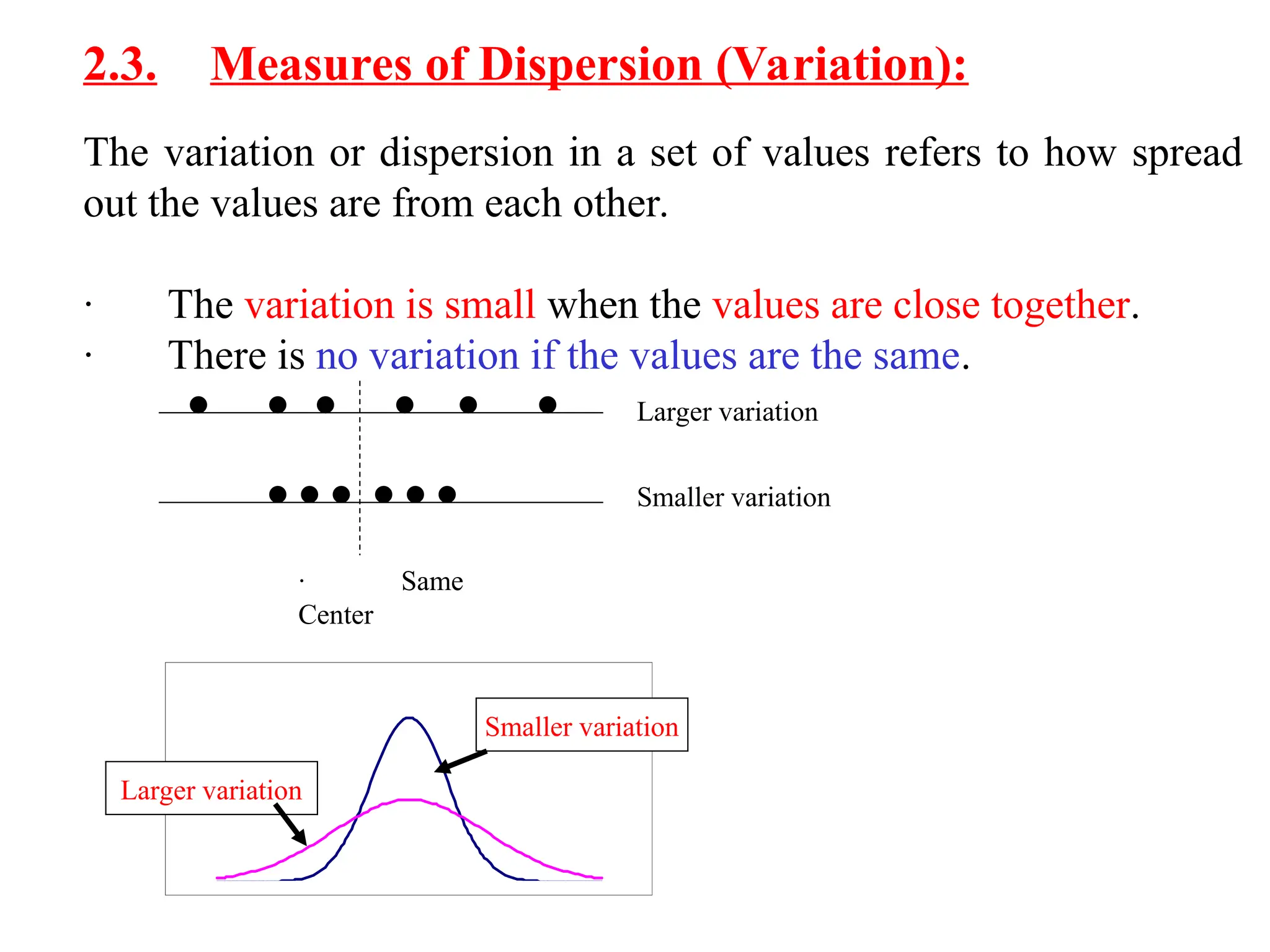
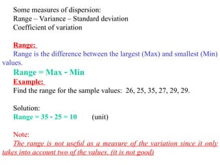
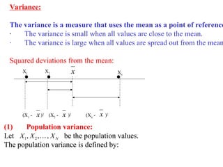
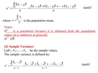
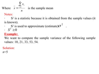
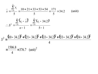
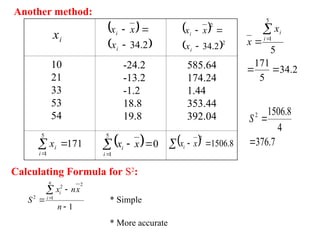
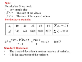
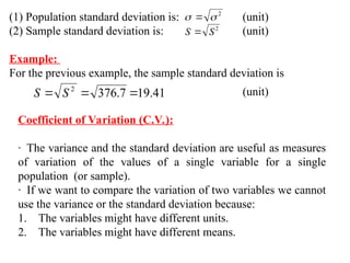
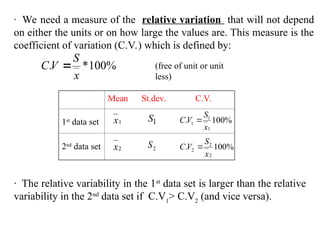
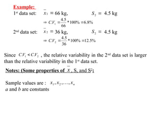
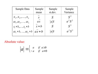
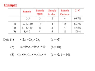
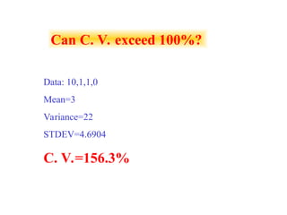
Larger variation
2.3. Measures of Dispersion (Variation):
The variation or dispersion in a set of values refers to how spread
out the values are from each other.
· The variation is small when the values are close together.
· There is no variation if the values are the same.
· Same
Center
Smaller variation
Smaller variation
Larger variation
Some measures of dispersion:
Range – Variance – Standard deviation
Coefficient of variation
Range:
Range is the difference between the largest (Max) and smallest (Min)
values.
Range = Max  Min
Example:
Find the range for the sample values: 26, 25, 35, 27, 29, 29.
Solution:
Range = 35  25 = 10 (unit)
Note:
The range is not useful as a measure of the variation since it only
takes into account two of the values. (it is not good)
Variance:
The variance is a measure that uses the mean as a point of reference
· The variance is small when all values are close to the mean.
· The variance is large when all values are spread out from the mean
Squared deviations from the mean:
X1
X2 x Xn
(X1
 )2
x (X2
 )2
x (Xn
 )2
x
(1) Population variance:
Let be the population values.
The population variance is defined by:
N
X
X
X ,
,
, 2
1 
       
N
X
X
X
N
X
N
N
i
i 2
2
2
2
1
1
2
2 














  (unit)2
where is the population mean.
N
X
N
i
i


 1

Notes:
· is a parameter because it is obtained from the population
values (it is unknown in general).
·
(2) Sample Variance:
Let be the sample values.
The sample variance is defined by:
2

0
2


n
x
x
x ,
,
, 2
1 
       
1
1
2
2
2
2
1
1
2
2













n
x
x
x
x
x
x
n
x
x
S N
n
i
i
 (unit)2
Where is the sample mean
n
x
x
n
i
i


 1
Notes:
· S2
is a statistic because it is obtained from the sample values (it
is known).
· S2
is used to approximate (estimate) .
·
Example:
We want to compute the sample variance of the following sample
values: 10, 21, 33, 53, 54.
2

0
2

S
Solution:
n=5
2
.
34
5
171
5
54
53
33
21
10
5
5
1










i
i
x
x (unit)
   
1
5
2
.
34
1
5
1
2
1
2
2










 i
i
n
i
i x
n
x
x
S
         
(unit)
7
.
376
4
8
.
1506
4
2
.
34
54
2
.
34
53
2
.
34
33
2
.
34
21
2
.
34
10
2
2
2
2
2
2
2












S
Another method:
 




5
1
0
i
i x
x  
 
 8
.
1506
2
x
xi
i
x  
 
2
.
34



i
i
x
x
x  
 2
2
2
.
34



i
i
x
x
x
-24.2
-13.2
-1.2
18.8
19.8
10
21
33
53
54
585.64
174.24
1.44
353.44
392.04



5
1
171
i
i
x
2
.
34
5
171
5
5
1





i
i
x
x
7
.
376
4
8
.
1506
2


S
Calculating Formula for S2
:
1
1
2
2
2





n
x
n
x
S
n
i
i
* Simple
* More accurate
Note:
To calculate S2
we need:
· n = sample size
· The sum of the values
· The sum of the squared values
For the above example:
 
i
x
 
2
i
x
10 21 33 53 54
100 441 1089 2809 2916
i
x
2
i
x
 171
i
x
 7355
2
i
x
   7
.
376
4
8
.
1506
1
5
2
.
34
5
7355
2
2





S (unit)2
Standard Deviation:
· The standard deviation is another measure of variation.
· It is the square root of the variance.
(1) Population standard deviation is: (unit)
(2) Sample standard deviation is: (unit)
Example:
For the previous example, the sample standard deviation is
2

 
2
S
S 
41
.
19
7
.
376
2


 S
S (unit)
Coefficient of Variation (C.V.):
· The variance and the standard deviation are useful as measures
of variation of the values of a single variable for a single
population (or sample).
· If we want to compare the variation of two variables we cannot
use the variance or the standard deviation because:
1. The variables might have different units.
2. The variables might have different means.
· We need a measure of the relative variation that will not depend
on either the units or on how large the values are. This measure is the
coefficient of variation (C.V.) which is defined by:
%
100
*
.
x
S
V
C  (free of unit or unit
less)
Mean St.dev. C.V.
%
100
.
1
1
1
x
S
V
C 
%
100
.
2
2
2
x
S
V
C 
1
S
1
x
2
x 2
S
1st
data set
2nd
data set
· The relative variability in the 1st
data set is larger than the relative
variability in the 2nd
data set if C.V1
> C.V2
(and vice versa).
Example:
1st
data set: 66 kg, 4.5 kg
2nd
data set: 36 kg, 4.5 kg

1
x

2
S
%
8
.
6
%
100
*
66
5
.
4
. 1 

 V
C

2
x

2
S
%
5
.
12
%
100
*
36
5
.
4
. 2 

 V
C
Since , the relative variability in the 2nd
data set is larger
than the relative variability in the 1st
data set.
2
1 .
. V
C
V
C 
Notes: (Some properties of , S, and S2
:
Sample values are :
a and b are constants
x
n
x
x
x ,
,
, 2
1 
Sample Data Sample
mean
Sample
st.dev.
Sample
Variance
n
x
x
x ,
,
, 2
1 
n
ax
ax
ax ,
,
, 2
1 
b
x
b
x n 
 ,
,
,
1 
b
ax
b
ax n 
 ,
,
1 
x
x
a
b
x 
b
x
a 
S
S
a
S
S
a
2
S
2
2
S
a
2
S
2
2
S
a
Absolute value:
 0
0



 a
if
a
a
if
a
a
Sample Sample
mean
Sample
St..dev.
Sample
Variance
C. V.
1,3,5 3 2 4 66.7%
(1)
(2)
(3)
-2, -6, -10
11, 13, 15
8, 4, 0
-6
13
4
4
2
4
16
4
16
66.7%
15.4%
100%
Example:
Data (1) (a = 2)
(2) (b = 10)
(3) (a = 2, b = 10)
3
2
1 2
,
2
,
2 x
x
x 


10
x
,
10
x
,
10
x 3
2
1 


10
x
2
,
10
x
2
,
10
x
2 3
2
1 





Can C. V. exceed 100%?
Data: 10,1,1,0
Mean=3
Variance=22
STDEV=4.6904
C. V.=156.3%

STANDARD DEVIATION SLIDESHOW OF LEOPOLDO

  • 1.
    Larger variation 2.3. Measuresof Dispersion (Variation): The variation or dispersion in a set of values refers to how spread out the values are from each other. · The variation is small when the values are close together. · There is no variation if the values are the same. · Same Center Smaller variation Smaller variation Larger variation
  • 2.
    Some measures ofdispersion: Range – Variance – Standard deviation Coefficient of variation Range: Range is the difference between the largest (Max) and smallest (Min) values. Range = Max  Min Example: Find the range for the sample values: 26, 25, 35, 27, 29, 29. Solution: Range = 35  25 = 10 (unit) Note: The range is not useful as a measure of the variation since it only takes into account two of the values. (it is not good)
  • 3.
    Variance: The variance isa measure that uses the mean as a point of reference · The variance is small when all values are close to the mean. · The variance is large when all values are spread out from the mean Squared deviations from the mean: X1 X2 x Xn (X1  )2 x (X2  )2 x (Xn  )2 x (1) Population variance: Let be the population values. The population variance is defined by: N X X X , , , 2 1 
  • 4.
           N X X X N X N N i i 2 2 2 2 1 1 2 2                  (unit)2 where is the population mean. N X N i i    1  Notes: · is a parameter because it is obtained from the population values (it is unknown in general). · (2) Sample Variance: Let be the sample values. The sample variance is defined by: 2  0 2   n x x x , , , 2 1          1 1 2 2 2 2 1 1 2 2              n x x x x x x n x x S N n i i  (unit)2
  • 5.
    Where is thesample mean n x x n i i    1 Notes: · S2 is a statistic because it is obtained from the sample values (it is known). · S2 is used to approximate (estimate) . · Example: We want to compute the sample variance of the following sample values: 10, 21, 33, 53, 54. 2  0 2  S Solution: n=5
  • 6.
    2 . 34 5 171 5 54 53 33 21 10 5 5 1           i i x x (unit)    1 5 2 . 34 1 5 1 2 1 2 2            i i n i i x n x x S           (unit) 7 . 376 4 8 . 1506 4 2 . 34 54 2 . 34 53 2 . 34 33 2 . 34 21 2 . 34 10 2 2 2 2 2 2 2             S
  • 7.
    Another method:       5 1 0 i ix x      8 . 1506 2 x xi i x     2 . 34    i i x x x    2 2 2 . 34    i i x x x -24.2 -13.2 -1.2 18.8 19.8 10 21 33 53 54 585.64 174.24 1.44 353.44 392.04    5 1 171 i i x 2 . 34 5 171 5 5 1      i i x x 7 . 376 4 8 . 1506 2   S Calculating Formula for S2 : 1 1 2 2 2      n x n x S n i i * Simple * More accurate
  • 8.
    Note: To calculate S2 weneed: · n = sample size · The sum of the values · The sum of the squared values For the above example:   i x   2 i x 10 21 33 53 54 100 441 1089 2809 2916 i x 2 i x  171 i x  7355 2 i x    7 . 376 4 8 . 1506 1 5 2 . 34 5 7355 2 2      S (unit)2 Standard Deviation: · The standard deviation is another measure of variation. · It is the square root of the variance.
  • 9.
    (1) Population standarddeviation is: (unit) (2) Sample standard deviation is: (unit) Example: For the previous example, the sample standard deviation is 2    2 S S  41 . 19 7 . 376 2    S S (unit) Coefficient of Variation (C.V.): · The variance and the standard deviation are useful as measures of variation of the values of a single variable for a single population (or sample). · If we want to compare the variation of two variables we cannot use the variance or the standard deviation because: 1. The variables might have different units. 2. The variables might have different means.
  • 10.
    · We needa measure of the relative variation that will not depend on either the units or on how large the values are. This measure is the coefficient of variation (C.V.) which is defined by: % 100 * . x S V C  (free of unit or unit less) Mean St.dev. C.V. % 100 . 1 1 1 x S V C  % 100 . 2 2 2 x S V C  1 S 1 x 2 x 2 S 1st data set 2nd data set · The relative variability in the 1st data set is larger than the relative variability in the 2nd data set if C.V1 > C.V2 (and vice versa).
  • 11.
    Example: 1st data set: 66kg, 4.5 kg 2nd data set: 36 kg, 4.5 kg  1 x  2 S % 8 . 6 % 100 * 66 5 . 4 . 1    V C  2 x  2 S % 5 . 12 % 100 * 36 5 . 4 . 2    V C Since , the relative variability in the 2nd data set is larger than the relative variability in the 1st data set. 2 1 . . V C V C  Notes: (Some properties of , S, and S2 : Sample values are : a and b are constants x n x x x , , , 2 1 
  • 12.
    Sample Data Sample mean Sample st.dev. Sample Variance n x x x, , , 2 1  n ax ax ax , , , 2 1  b x b x n   , , , 1  b ax b ax n   , , 1  x x a b x  b x a  S S a S S a 2 S 2 2 S a 2 S 2 2 S a Absolute value:  0 0     a if a a if a a
  • 13.
    Sample Sample mean Sample St..dev. Sample Variance C. V. 1,3,53 2 4 66.7% (1) (2) (3) -2, -6, -10 11, 13, 15 8, 4, 0 -6 13 4 4 2 4 16 4 16 66.7% 15.4% 100% Example: Data (1) (a = 2) (2) (b = 10) (3) (a = 2, b = 10) 3 2 1 2 , 2 , 2 x x x    10 x , 10 x , 10 x 3 2 1    10 x 2 , 10 x 2 , 10 x 2 3 2 1      
  • 14.
    Can C. V.exceed 100%? Data: 10,1,1,0 Mean=3 Variance=22 STDEV=4.6904 C. V.=156.3%