Machine learning learning based frequency item sets definition types concepts

1. ML Based on Frequent Itemsets
CHAPTER 5: MACHINE LEARNING – THEORY & PRACTICE

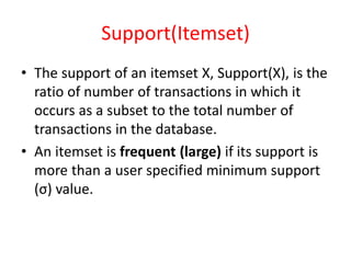
2. Support(Itemset)
• The support of an itemset X, Support(X), is the
ratio of number of transactions in which it
occurs as a subset to the total number of
transactions in the database.
• An itemset is frequent (large) if its support is
more than a user specified minimum support
(σ) value.

3. Association Rule
• An association rule is an expression of the
form A ⇒ C, where A and C are sets of items.
Left hand side of the rule (A) is called the
antecedent and the right hand side of the rule
(C) is called the consequent.
• Every association rule must satisfy two user
specified constraints, one is support (σ) and
the other is confidence(c).

4. Association Rule (Contd.)
• Support of the rule A ⇒ C is defined as the
fraction of tuples that contain both A and C. In
other words, it is the Support(A ∪ C).
• Confidence of the rule is defined as Support(A
∪ C) / Support(A).
• The goal is to find all rules that satisfy
minimum support and minimum confidence
specified by the user.

5. Mining of Association Rules
Definition :
A  B, A,B – Set of items.
➢ Support : Count (A  B)
➢ Confidence factor : Count (A  B)
Count (A)
A General block diagram :
Frequent/
Large itemsets
generator
Association rules
generator
Database Large Itemsets Association rules

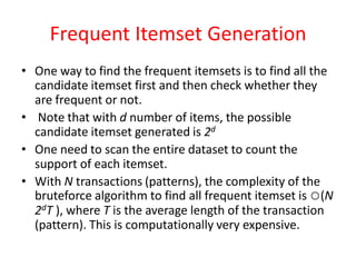
6. Frequent Itemset Generation
• One way to find the frequent itemsets is to find all the
candidate itemset first and then check whether they
are frequent or not.
• Note that with d number of items, the possible
candidate itemset generated is 2d
• One need to scan the entire dataset to count the
support of each itemset.
• With N transactions (patterns), the complexity of the
bruteforce algorithm to find all frequent itemset is ○(N
2dT ), where T is the average length of the transaction
(pattern). This is computationally very expensive.

7. Frequent Itemset Generation Strategies
• Reduce the number of candidates generated:
One can use a pruning technique to reduce
unnecessary candidate generation. Ex: Apriori
algorithm (discussed next).
• Reduce the number of comparisons: Only the
itemset which are relevant to the transaction
need to be compared. Ex: Frequent Pattern
(FP) tree based algorithm (discussed next).

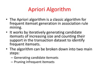
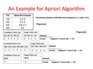
8. Apriori Algorithm
• The Apriori algorithm is a classic algorithm for
frequent itemset generation in association rule
mining.
• It works by iteratively generating candidate
itemsets of increasing size and counting their
support in the transaction dataset to identify
frequent itemsets.
• The algorithm can be broken down into two main
steps:
– Generating candidate itemsets
– Pruning infrequent itemsets

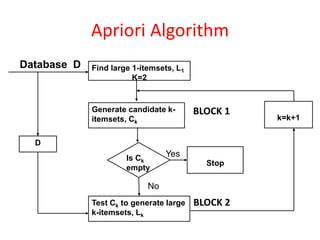
9. Apriori Algorithm
Database D Find large 1-itemsets, L1
K=2
Generate candidate k-
itemsets, Ck
D
Test Ck to generate large
k-itemsets, Lk
Is Ck
empty
Stop
k=k+1
Yes
No
BLOCK 1
BLOCK 2

10. Apriori Principle
• If an itemset is frequent, then all of its subsets
must also be frequent. This principle holds
due to the following property of support
measure:
∀X, Y : (X ⊆ Y ) ⇒ s(X) ≥ s(Y )
• Note that support of a set never exceeds its
subset. This property is also known as anti-
monotone property of support

11. An Example for Apriori Algorithm

12. Issues with Apriori Algorithm
• Generation of number of k-candidate itemsets
from large (k-1) itemsets.
– For example, with 104 large 1-itemsets, the number of
2-itemset candidates is about 107 which is large.
• Number of dataset or database scans. For large k-
itemsets, we need to scan the database (k+1)
times.
– With huge databases, each scan will take considerable
amount of time, thus making the apriori algorithm
computationally expensive.

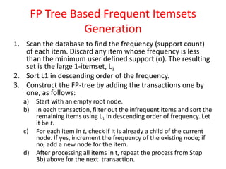
13. FP Tree Based Frequent Itemsets
Generation
1. Scan the database to find the frequency (support count)
of each item. Discard any item whose frequency is less
than the minimum user defined support (σ). The resulting
set is the large 1-itemset, L1
2. Sort L1 in descending order of the frequency.
3. Construct the FP-tree by adding the transactions one by
one, as follows:
a) Start with an empty root node.
b) In each transaction, filter out the infrequent items and sort the
remaining items using L1 in descending order of frequency. Let
it be t.
c) For each item in t, check if it is already a child of the current
node. If yes, increment the frequency of the existing node; if
no, add a new node for the item.
d) After processing all items in t, repeat the process from Step
3b) above for the next transaction.

14. FP Tree Based Frequent Itemsets
Generation (Contd.)
4. For each frequent item in L1, starting from the least frequent item,
construct its conditional pattern base and conditional FP-tree as follows:
a) Starting from the bottom of the FP-tree, trace the path from the item
node to the root node, and for each node on the path (excluding the
item node itself), collect the set of items in the path as well as the
frequency of the node.
b) Consider the item node and its corresponding transactions from the
FP-tree to obtain the conditional pattern base.
c) Construct the conditional FP-tree by applying the same steps as in
the main FP-tree construction algorithm, but using the conditional
pattern base as the input database.
5. Recursively mine the conditional FP-tree for each frequent item to
generate all frequent itemsets containing the current itemset and the
frequent item.
6. Remove the frequent item from the current itemset and repeat the
process with the next frequent item.
7. Combine all the frequent itemsets obtained from the recursive mining
of the conditional FP-trees to obtain the final set of frequent itemsets

15. An Example for FP Tree Based
Frequent Itemset Generation

16. Pattern Count (PC) Tree Based
Frequent Itemset Generation
• Construction of a PC-tree
– Construct the root of PC-tree, T .
– For each transaction, t in the transaction database, DB :
– Begin
• prnt = T
• For each item i in t :
• Begin
– If any one of the child nodes say, chld of prnt has item-name = item number of i
» Increment the count field value of chld.
» Set prnt = chld.
– Else
» Create a new node, nw.
» Set item-name field of nw to item-number of i.
» Set Count field of nw to 1.
» Attach nw as one of the child nodes of prnt.
» Set prnt = nw.
• End.
– End.

17. Tree Structures for Storing Patterns

18. Differences between FPT and PCT
• Typically, the number of nodes in an FP-tree is smaller than
the number of nodes in the corresponding PC-tree. In
previous example, the PC-tree has 20 nodes and the
corresponding FP-tree has only 12 nodes.
• Since PC-tree is a complete representation (i.e., non-lossy)
of the database, it can be used for dynamic mining (i.e.,
mining in change of data, knowledge and other mining
parameters scenario). However, the FP-tree is not a
complete (i.e., lossy) representation of the database as it is
based on frequent 1-itemsets. As a consequence, it is not
suited for dynamic mining.
• The number of database scans to construct the PC-tree is 1,
where as it is 2 in the case of FP-tree

19. Dynamic Mining
⚫ Change of data
– Addition
– Deletion
– Modification
⚫ Change of knowledge
⚫ Change of support value
} Incrementally

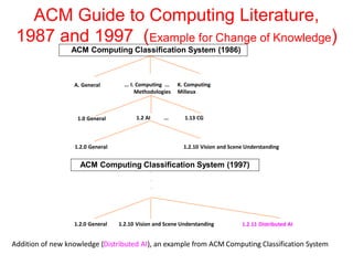
20. ACM Guide to Computing Literature,
1987 and 1997 (Example for Change of Knowledge)
ACM Computing Classification System (1986)
A. General ... I. Computing ... K. Computing
Methodologies Milieux
1.0 General 1.2 AI ... 1.13 CG
1.2.0 General 1.2.10 Vision and Scene Understanding
ACM Computing Classification System (1997)
.
.
.
1.2.0 General 1.2.10 Vision and Scene Understanding 1.2.11 Distributed AI
Addition of new knowledge (Distributed AI), an example from ACM Computing Classification System

21. Classification Rule Mining
• Let D is the dataset, I is the set of all items in D, and Y is the
set of class labels.
• A class association rule (CAR) follows the form X ⇒ y, where
X belongs to I and y belongs to Y .
• A rule X ⇒ y is said to hold in D with a confidence of c% if
c% of the cases in D that contain X are labeled with class y.
• The rule X ⇒ y has support s in D if s% of the cases in D
contain X and are labeled with class y.
• If the support of the CAR is greater than a user-defined
support (σ), the rule is considered frequent.
• If the confidence is greater than a user-defined confidence
(c), the rule is deemed accurate.

22. Example for CAR

23. Frequent Itemsets for Classification
using PC-tree (PC-Classifier)
• INPUTS :
– TS - Test dataset (A collection of test patterns.)
– TR - Training dataset (A collection of training patterns.)
• OUTPUTS :
– Ctime - Classification time.
– CA - Classification accuracy.
• STEPS :
– Generate PC-tree using TR (refer section 5.5.2 for details).
– start-time = time().
– For each si ∈ TS
• Find ni, set of positions of non-zero values corresponding to si.
• Find the nearest neighbour branch, ek in PC-tree depending on maximum number of features which
are common to both ek and ni.
• Attach the label l associated with ek to ni.
• If (l == label of si) then correct = correct + 1
– end-time = time().
– CA = correct
– |TS | × 100 // |TS | is the number of test patterns.
– Output Ctime = end-time - start-time.
– Output CA

24. An Example for PC-Classifier
The PC-tree is constructed using labelled training data and then, the test data is checked
against each path of PC-tree to determine its class label.

25. Frequent Itemsets for Clustering using
PC-tree (PC-Cluster)
• PC-tree based clustering algorithm (PC-Cluster)
• STORE :
– For each pattern, Pi ∈ D (database) :
– If any prefix sub pattern, SPi, of Pi exists as a prefix in a branch eb :
– Put features in SPi in eb, by incrementing the corresponding count field
value of the nodes in the PC-tree. Put the sub patterns, if any, of Pi by
appending additional nodes with count field value equal to 1 to the
path in eb.
– Else Put Pi as a new branch of the PC-tree.
• RETRIEVE :
– For each branch, Bi ∈ P C (PC-tree) :
• For each node, Nj ∈ Bi :
– Output Nj .Feature.
• The features corresponding to the nodes in the branch of the PC-
tree from root to leaf constitute a prototype.

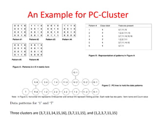
26. An Example for PC-Cluster
Three clusters are {3,7,11,14,15,16}, {3,7,11,15}, and {1,2,3,7,11,15}