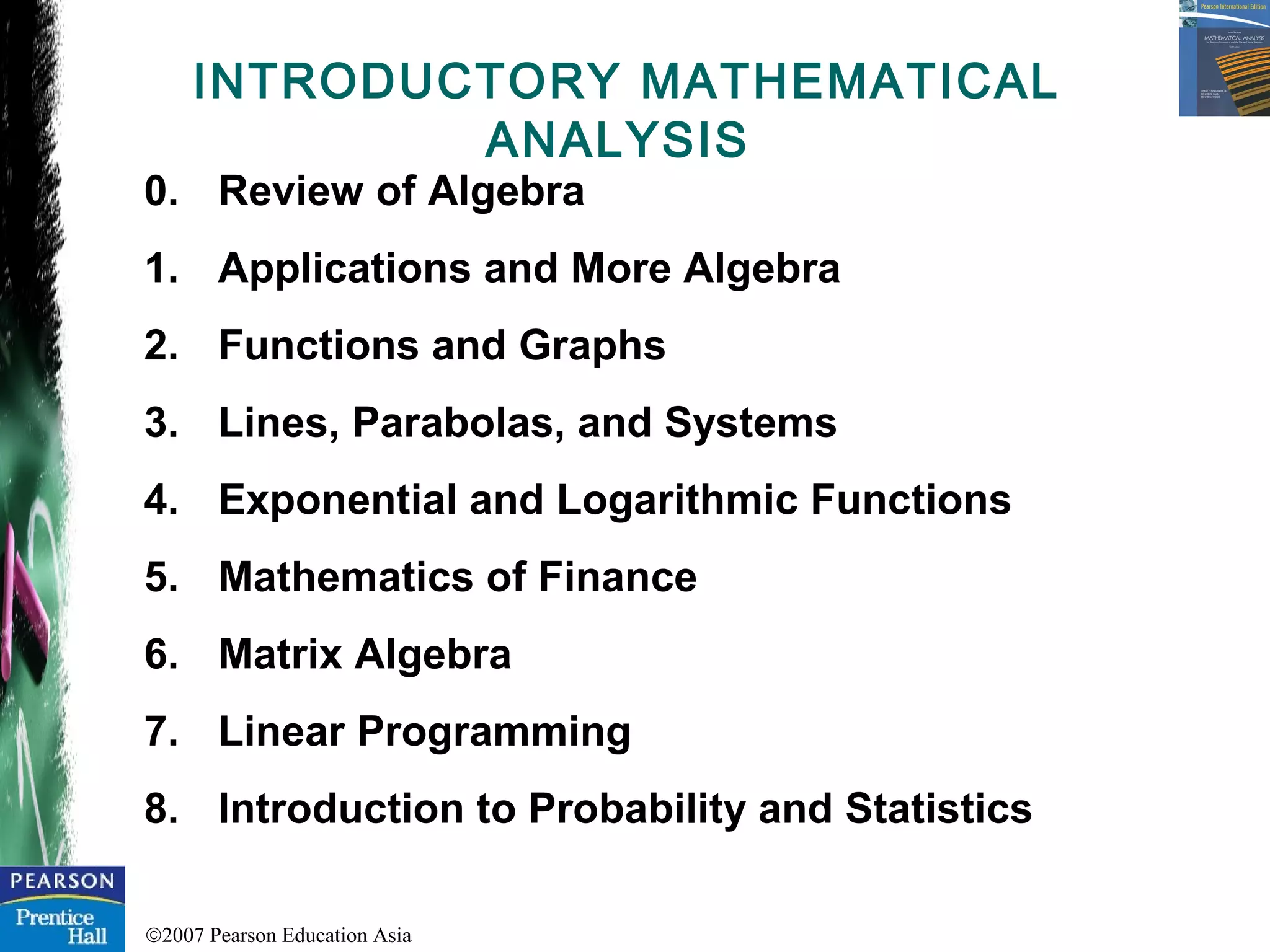
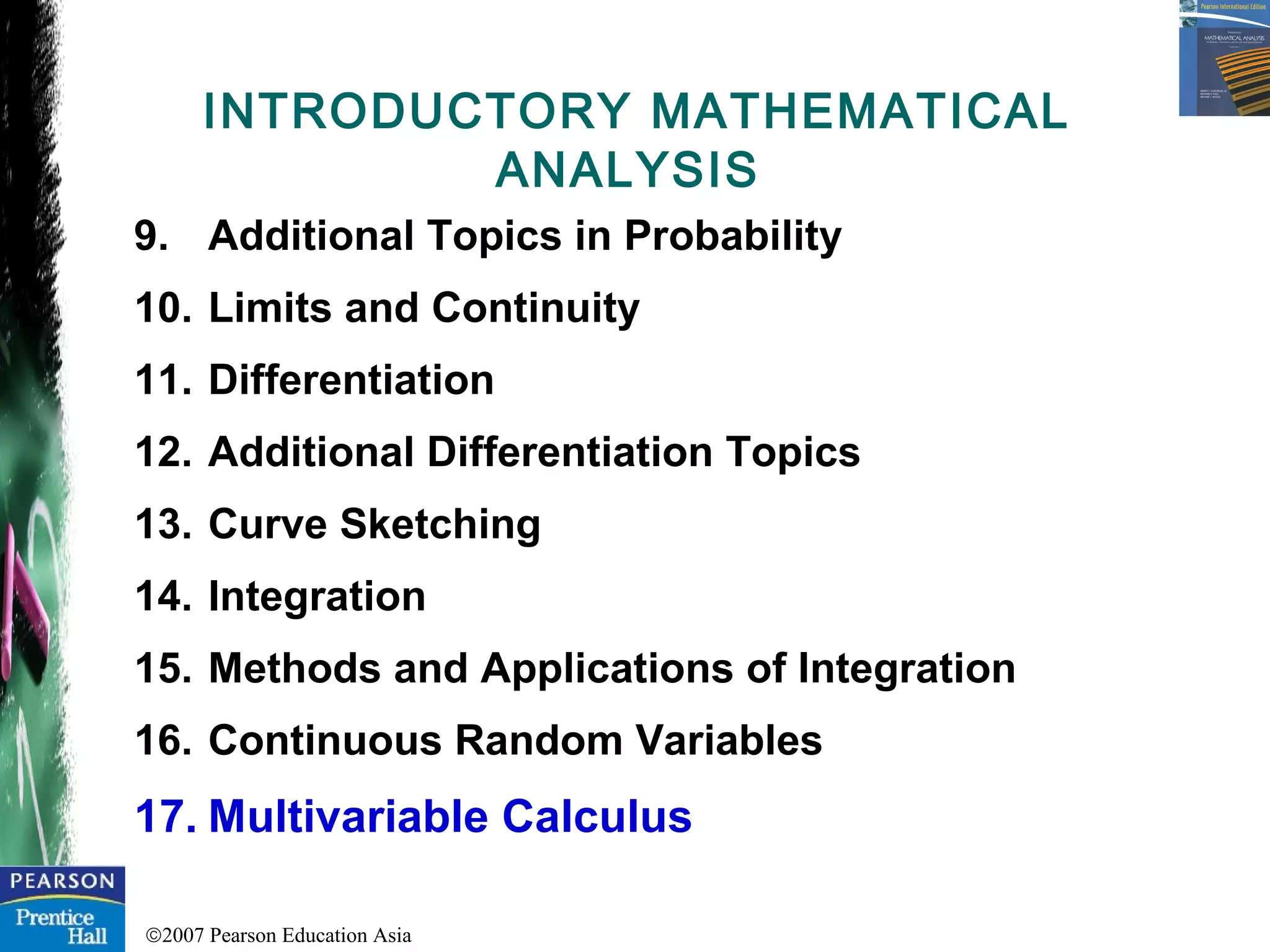
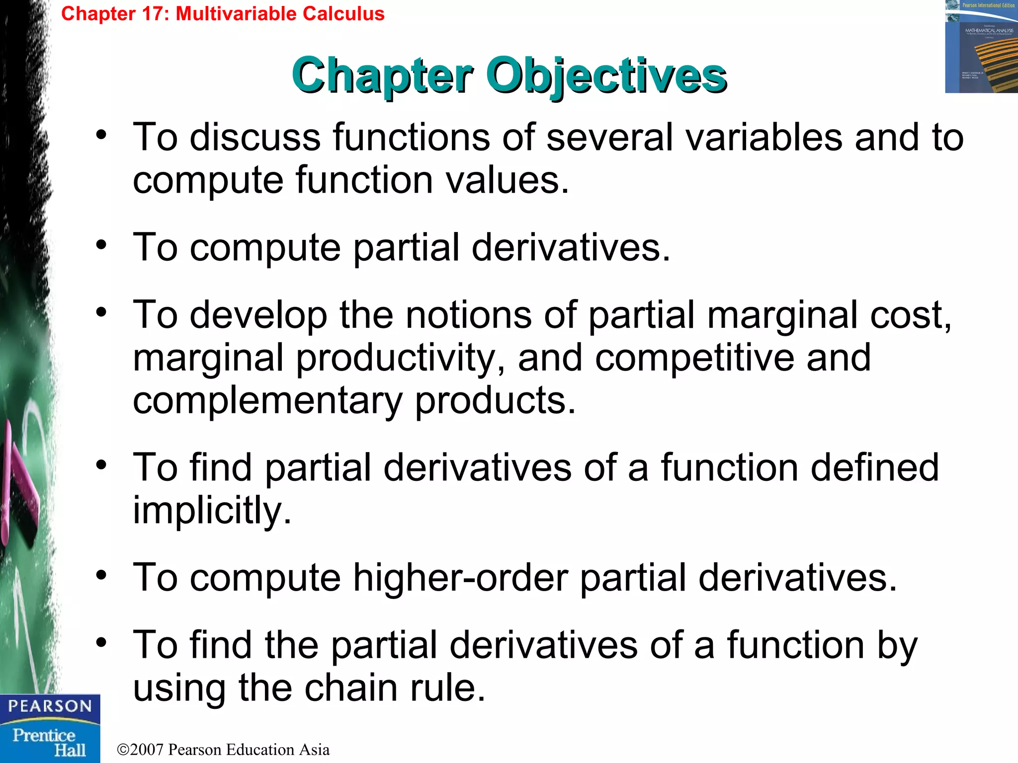
This chapter discusses multivariable calculus topics including functions of several variables, partial derivatives, applications of partial derivatives, implicit partial differentiation, higher-order partial derivatives, the chain rule, and finding maxima and minima for functions of two variables. It provides examples of computing partial derivatives, finding marginal costs and productivity, implicit partial differentiation, and using the chain rule. The objectives are to develop concepts and techniques for multivariable calculus including computing partial derivatives and applying optimization methods.

![©2007 Pearson Education Asia
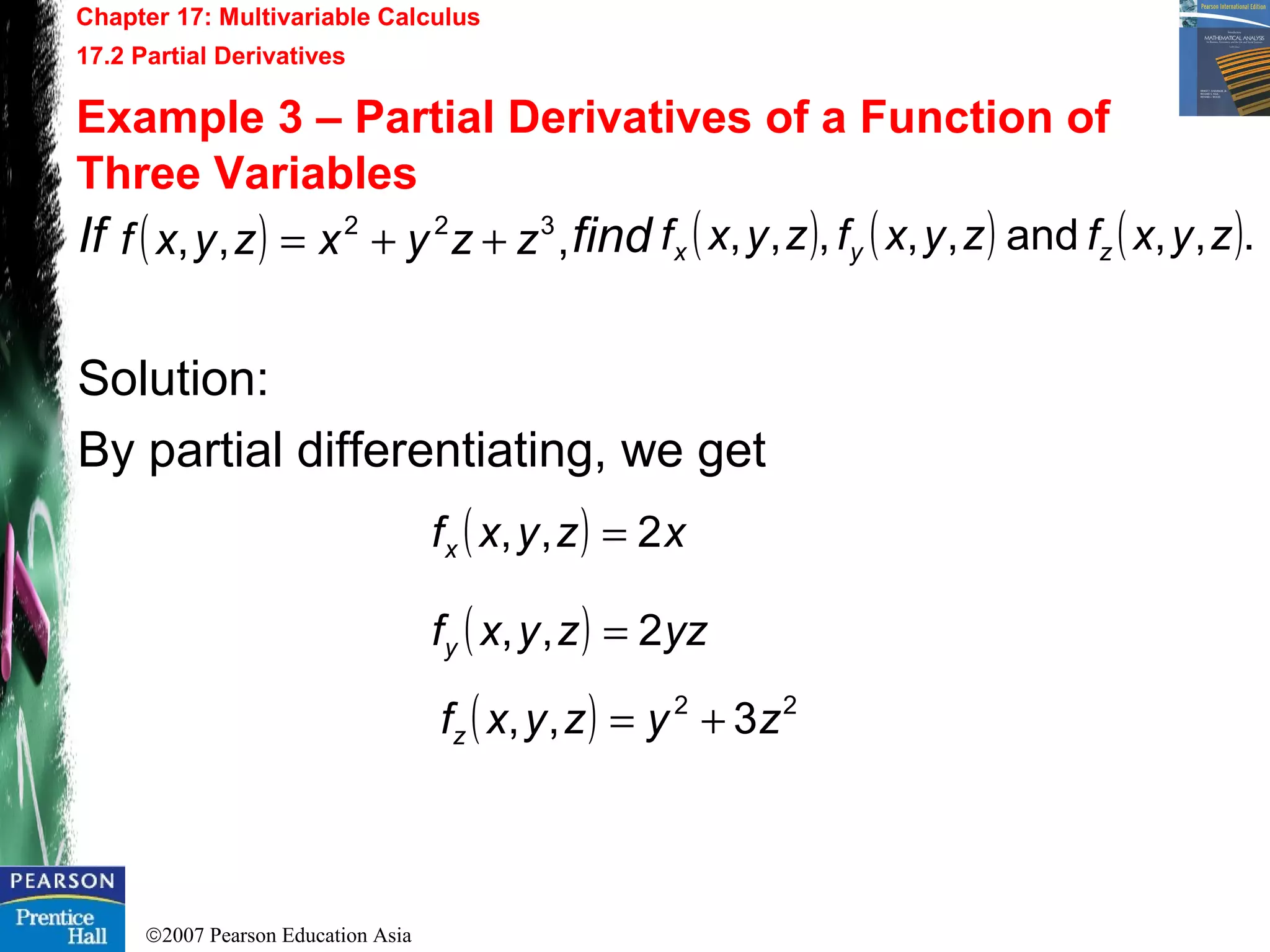
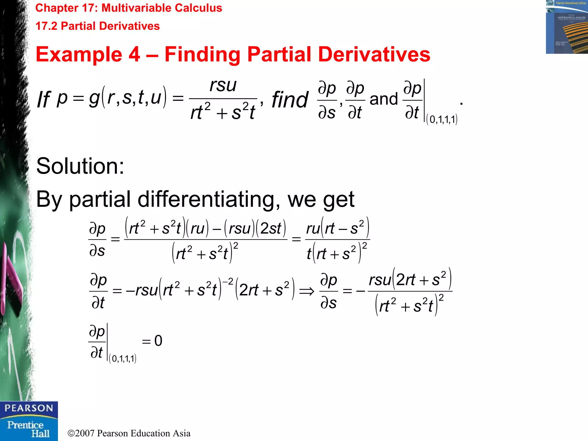
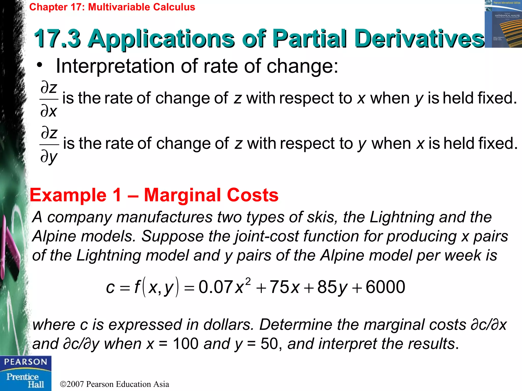
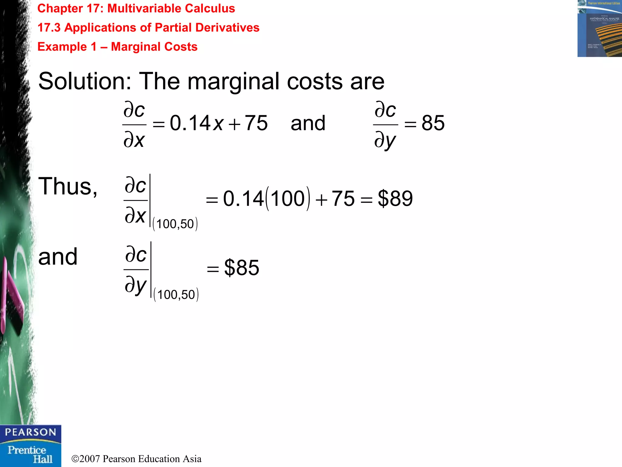
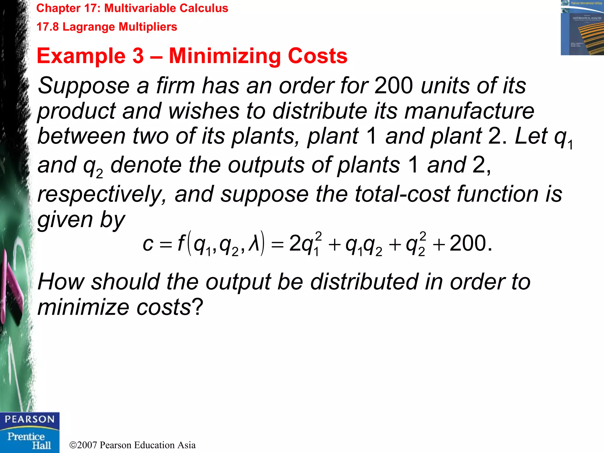
Chapter 17: Multivariable Calculus
17.10 Multiple Integrals17.10 Multiple Integrals
Example 1 – Evaluating a Double Integral
• Definite integrals of functions of two variables are
called (definite) double integrals, which involve
integration over a region in the plane.
Find
Solution:
( ) .12
1
1
1
0
dxdyx
x
∫ ∫−
−
+
( )
[ ]
3
2
23
2
2
12
1
1
231
1
1
0
1
1
1
0
=
++−=+=
+
−−
−
−
−
∫
∫ ∫
x
xx
dxyxy
dxdyx
x
x](https://image.slidesharecdn.com/chapter17-multivariablecalculus-151007044001-lva1-app6891-180205110412/75/Chapter17-multivariablecalculus-151007044001-lva1-app6891-40-2048.jpg)
![©2007 Pearson Education Asia
Chapter 17: Multivariable Calculus
17.10 Lines of Regression
Example 3 – Evaluating a Triple Integral
Find
Solution:
.
1
0 0 0
dxdydzx
x yx
∫∫ ∫
−
[ ]
8
1
82
1
0
41
0 0
2
2
1
0 0
0
1
0 0 0
=
=
−=
=
∫
∫∫∫∫ ∫
−
−
x
dx
xy
yx
dxdyxzdxdydzx
x
x
yx
x yx](https://image.slidesharecdn.com/chapter17-multivariablecalculus-151007044001-lva1-app6891-180205110412/75/Chapter17-multivariablecalculus-151007044001-lva1-app6891-41-2048.jpg)