Chapter 5: Theoryon producer behaviors
June 3, 2020
Microeconomics June 3, 2020 3 / 50
4.
Content
1 Theory ofproduction
Production function
Production with a variable input
Production with two variable inputs
2 Theory of cost
Short-run costs
Long-run costs
Economic cost, accounting cost, sunk cost
Microeconomics June 3, 2020 4 / 50
5.
Theory of production
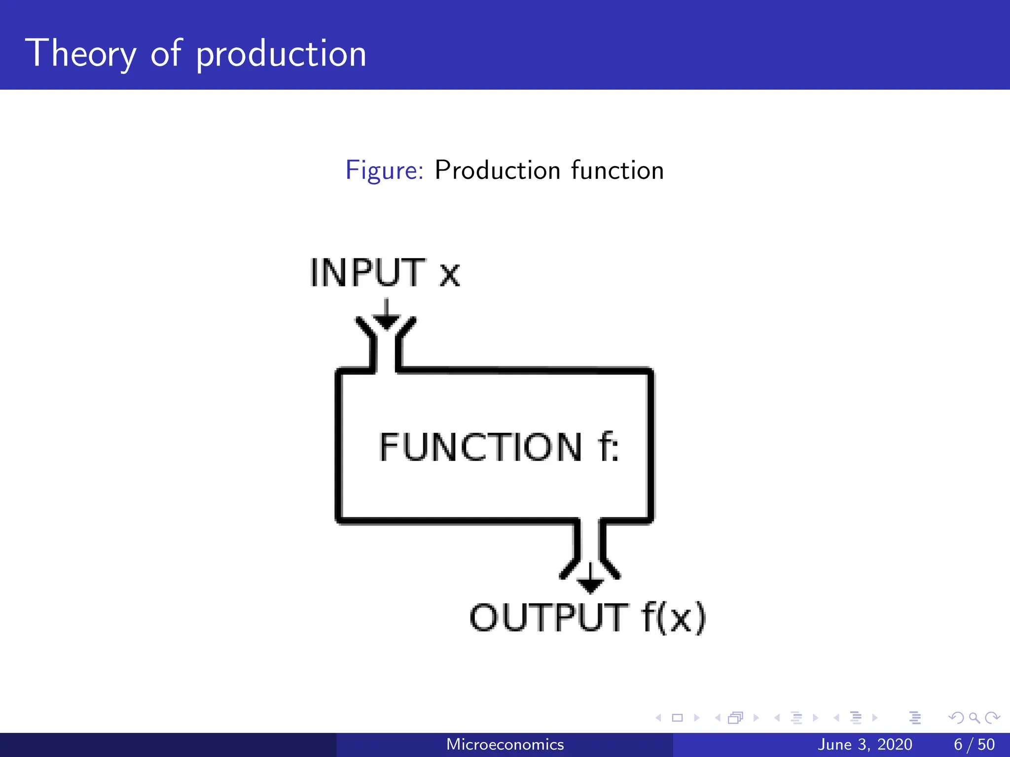
Productionfunction
A production function: Function showing the highest output that a firm
can produce for every specified combination of inputs applies to a given
technology.
Given technology is a given state of knowledge about the various methods
that might be used to transform inputs into outputs.
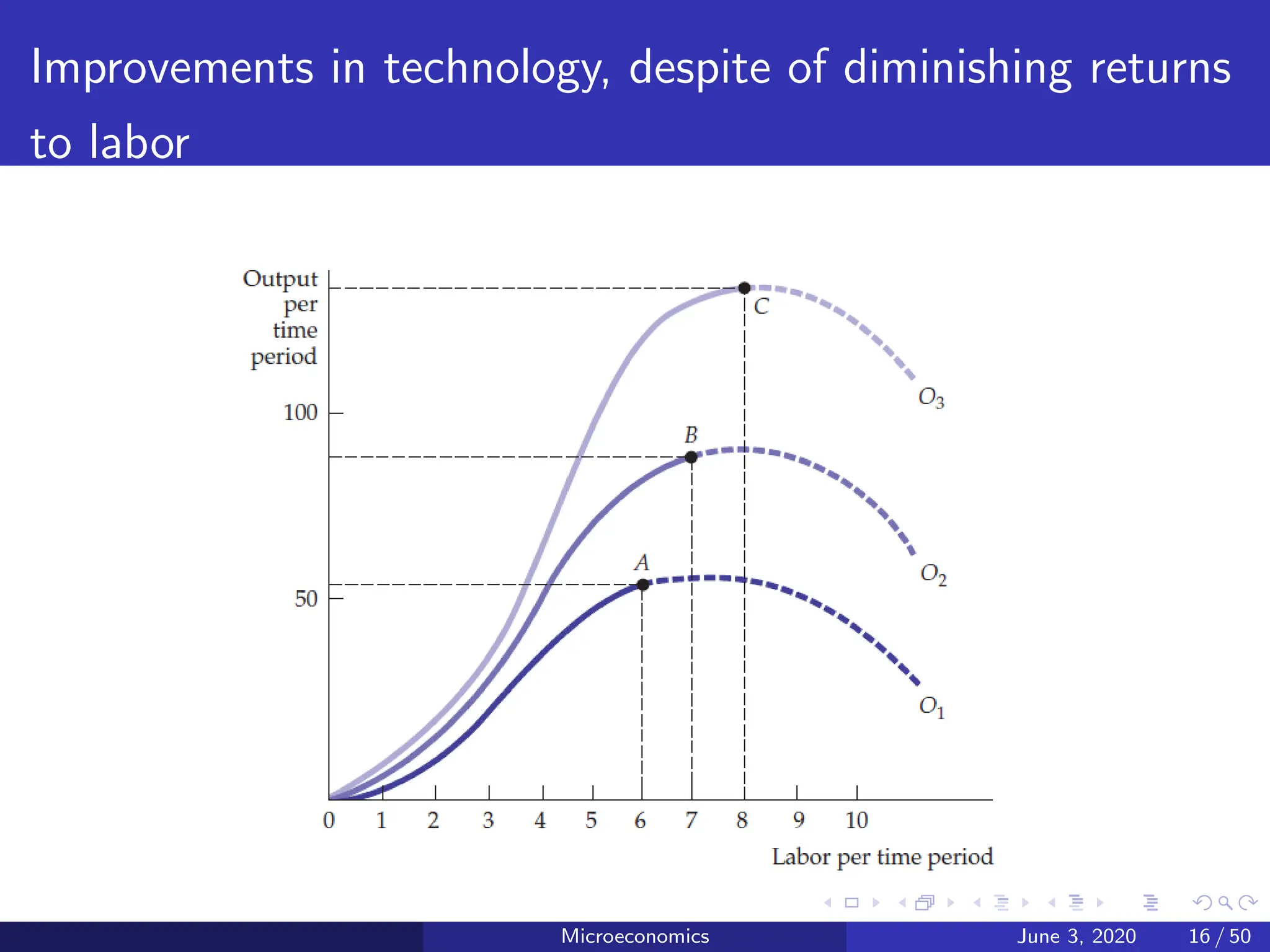
As the technology becomes more advanced and the production function
changes, a firm can obtain more output for a given set of inputs.
Microeconomics June 3, 2020 5 / 50
Theory of production
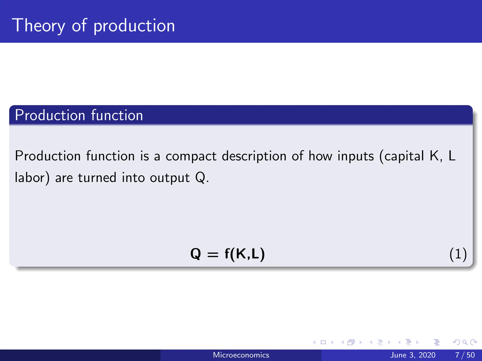
Productionfunction
Production function is a compact description of how inputs (capital K, L
labor) are turned into output Q.
Q = f(K,L) (1)
Microeconomics June 3, 2020 7 / 50
8.
Short-run versus Long-run
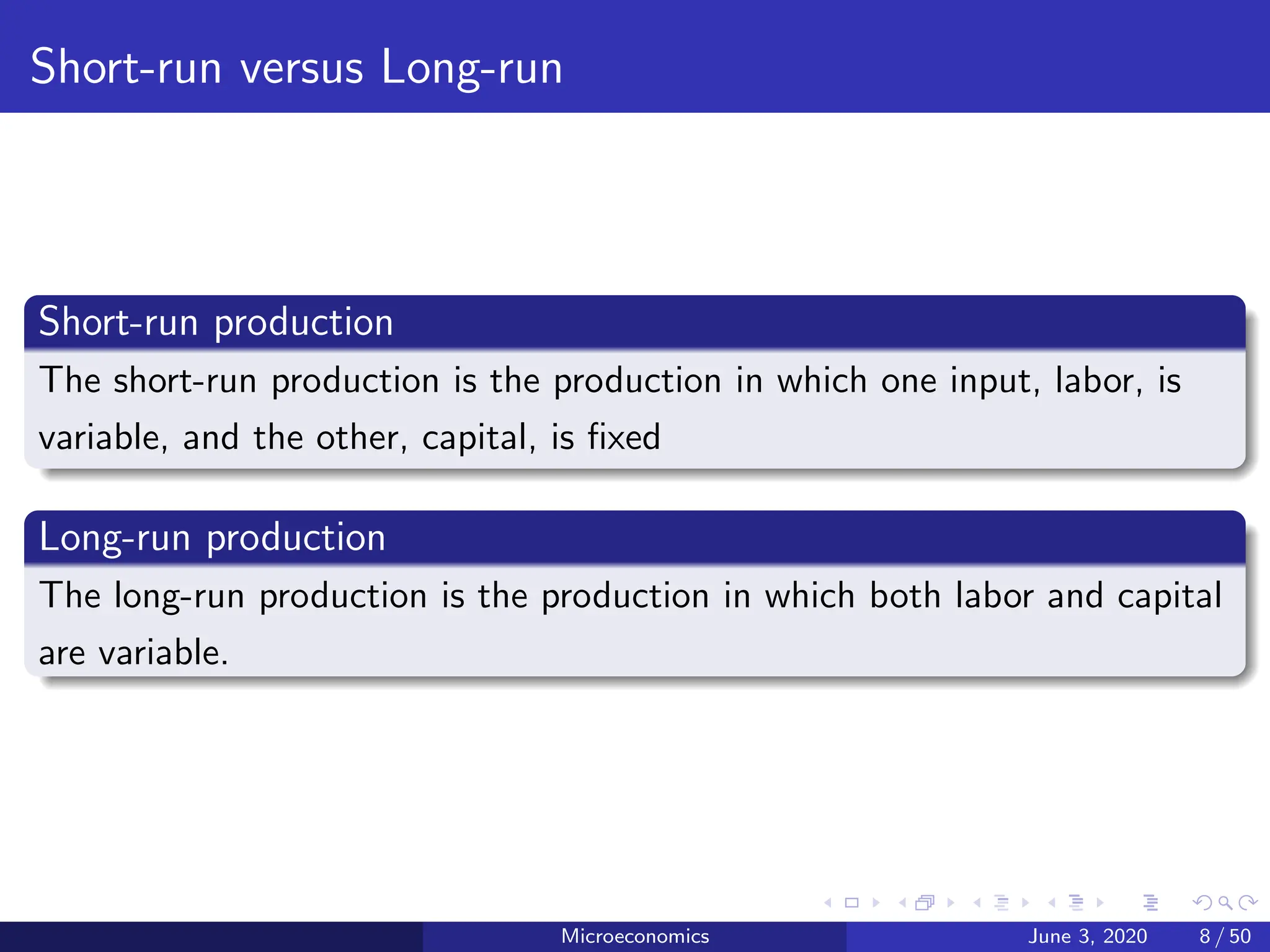
Short-runproduction
The short-run production is the production in which one input, labor, is
variable, and the other, capital, is fixed
Long-run production
The long-run production is the production in which both labor and capital
are variable.
Microeconomics June 3, 2020 8 / 50
9.
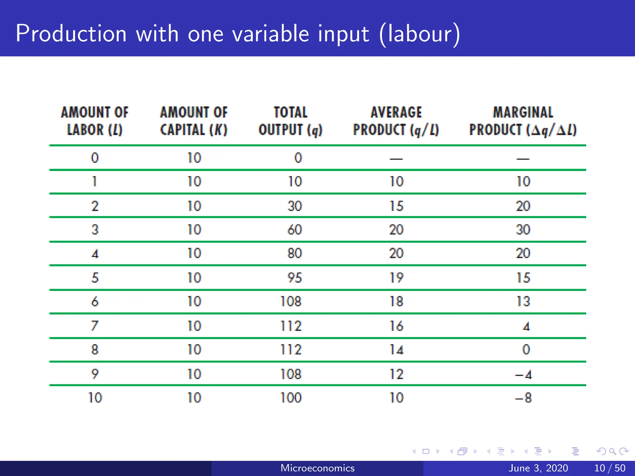
Production with onevariable input (labour)
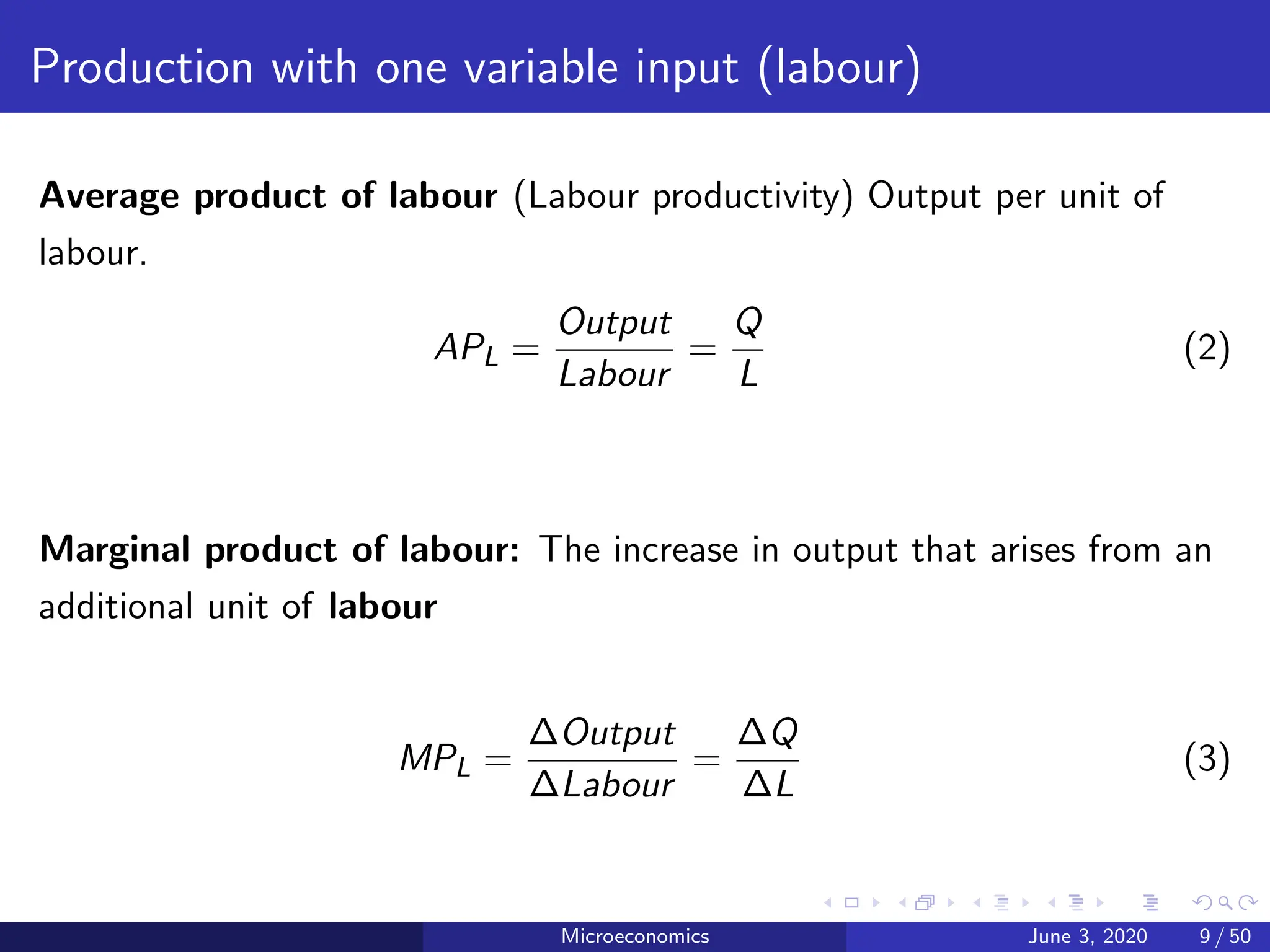
Average product of labour (Labour productivity) Output per unit of
labour.
APL =
Output
Labour
=
Q
L
(2)
Marginal product of labour: The increase in output that arises from an
additional unit of labour
MPL =
∆Output
∆Labour
=
∆Q
∆L
(3)
Microeconomics June 3, 2020 9 / 50
10.
Production with onevariable input (labour)
Microeconomics June 3, 2020 10 / 50
11.
Diminishing marginal product
Themarginal product of an input declines as the quantity of the
input increases
Explain: As the number of workers increases, additional workers
have to share equipment and work in more crowded conditions.
Microeconomics June 3, 2020 11 / 50
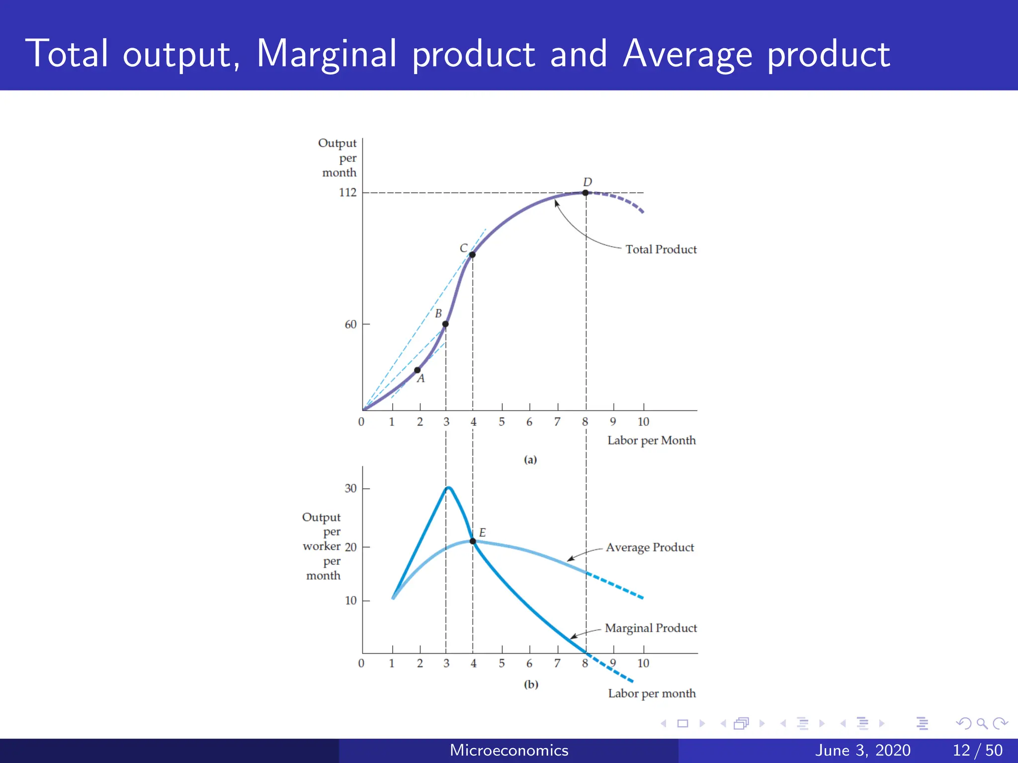
Total output, Marginalproduct and Average product
The marginal product is above the average product when the average
product is increasing and below the average product when the average
product is decreasing.
It follows, therefore, that the marginal product must equal the average
product when the average product reaches its maximum. This happens at
point E.
Microeconomics June 3, 2020 13 / 50
14.
The Law ofDiminishing Marginal Returns
Principle that as the use of an input increases with other inputs fixed,
the resulting additions to output will eventually decrease.
The law of diminishing marginal returns describes a declining marginal
product but not necessarily a negative one.
The law of diminishing marginal returns applies to a given production
technology
Microeconomics June 3, 2020 14 / 50
15.
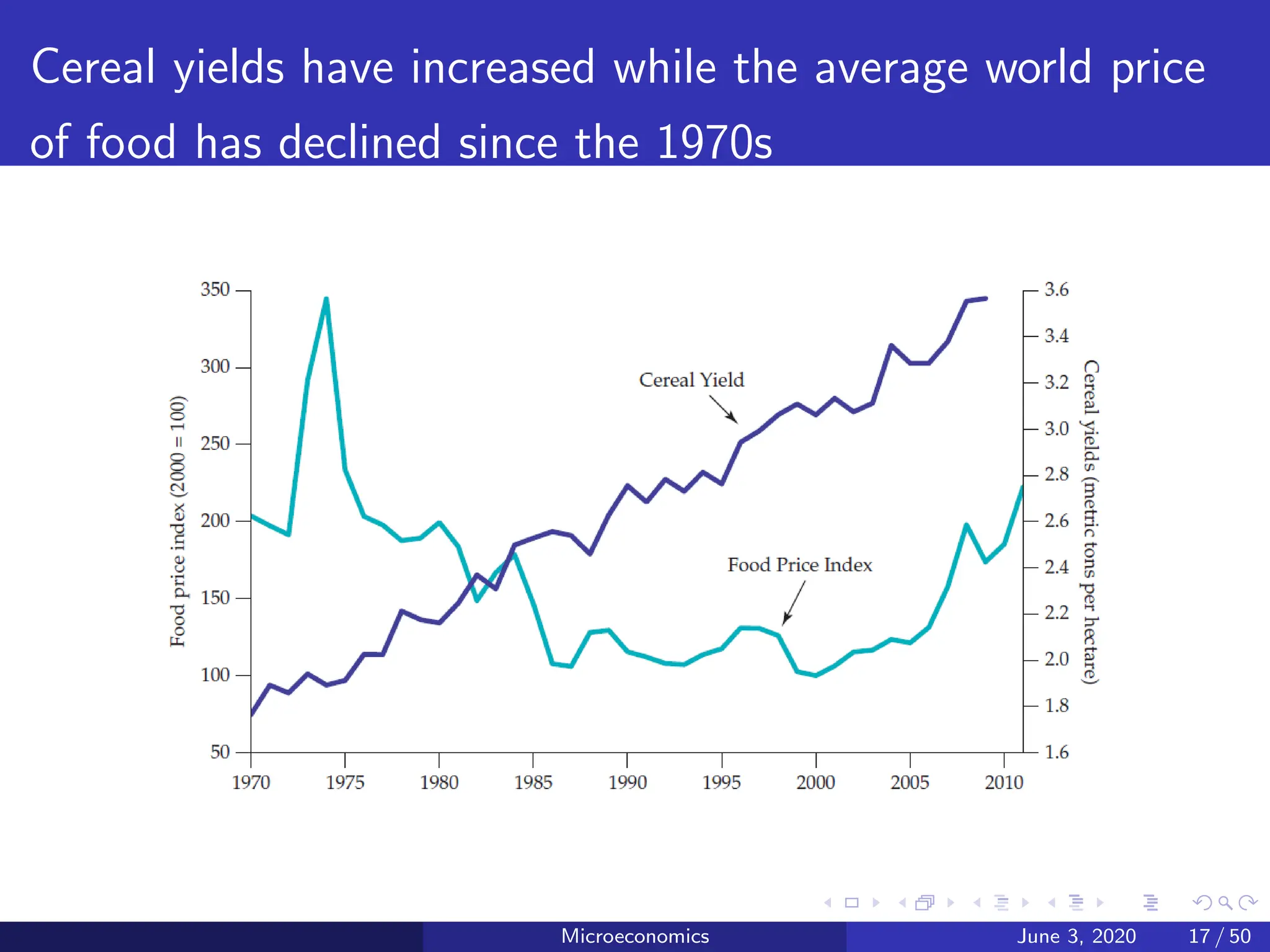
Is there foodcrisis?
Political economist Thomas Malthus (1766–1834) believed that the
world’s limited amount of land would not be able to supply enough food as
the population grew.
He predicted that as both the marginal and average productivity of labor
fell and there were more mouths to feed, mass hunger and starvation
would result.
Microeconomics June 3, 2020 15 / 50
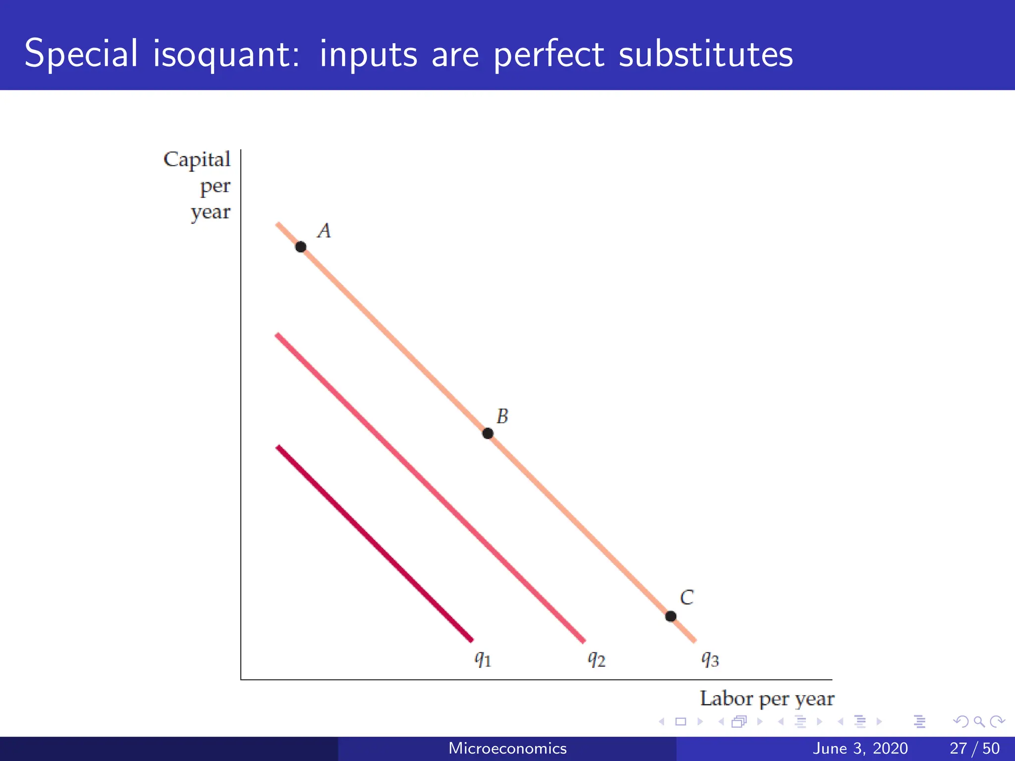
Production with twovariable inputs
Isoquant
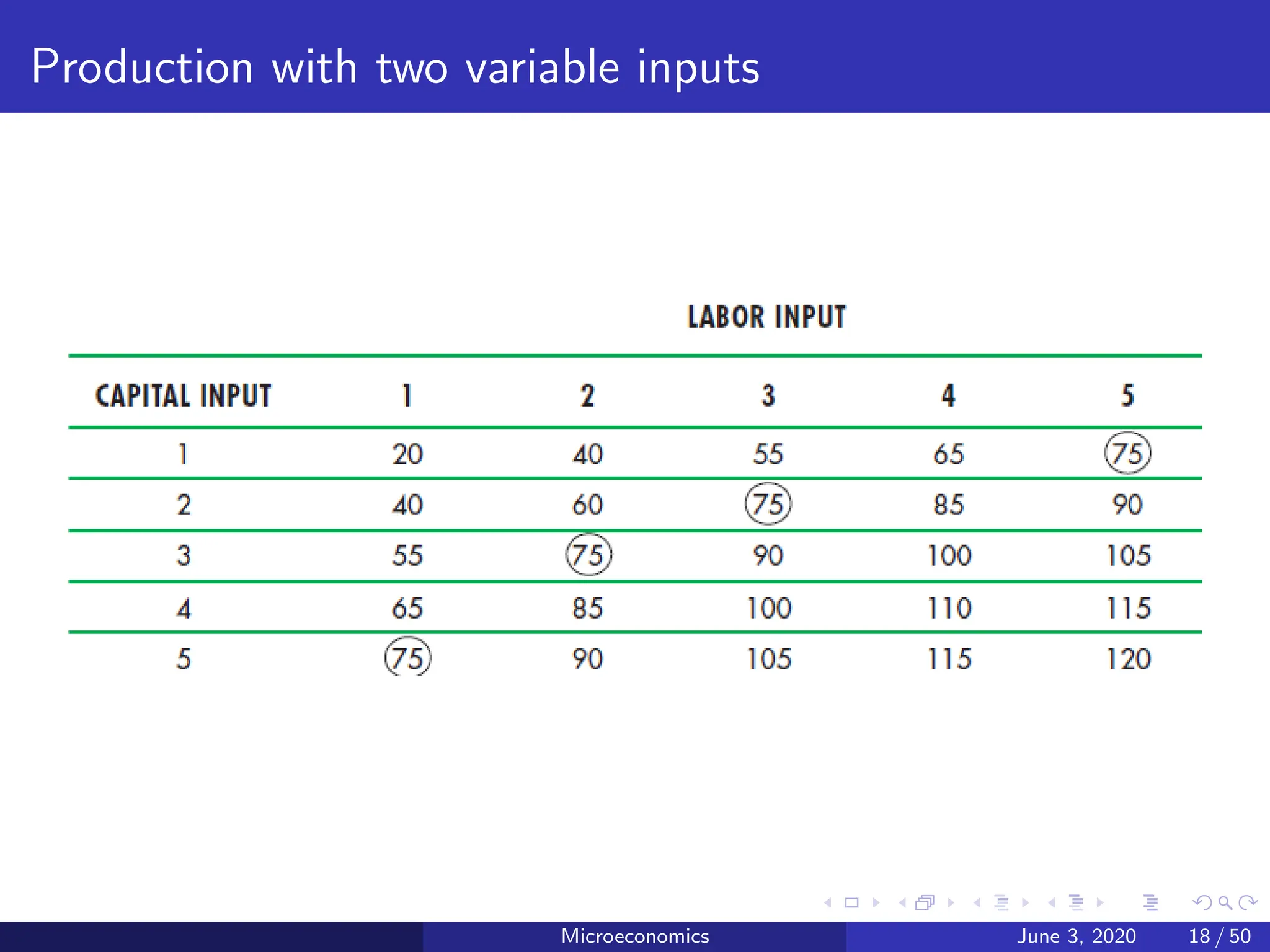
An isoquant is a curve that shows all the possible combinations of inputs
that yield the same output.
Microeconomics June 3, 2020 19 / 50
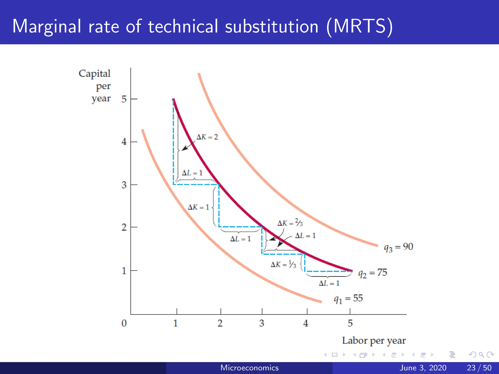
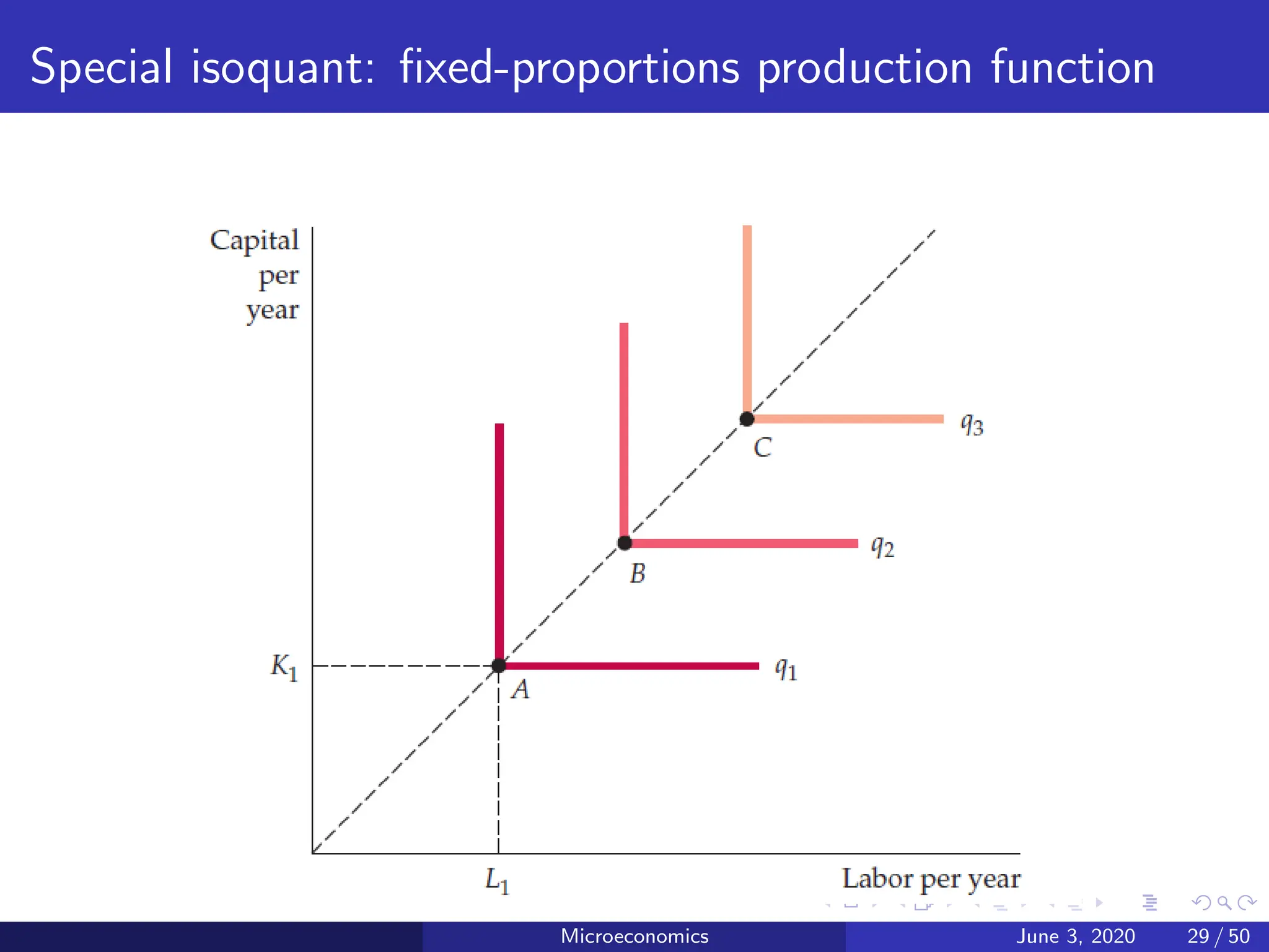
Isoquants
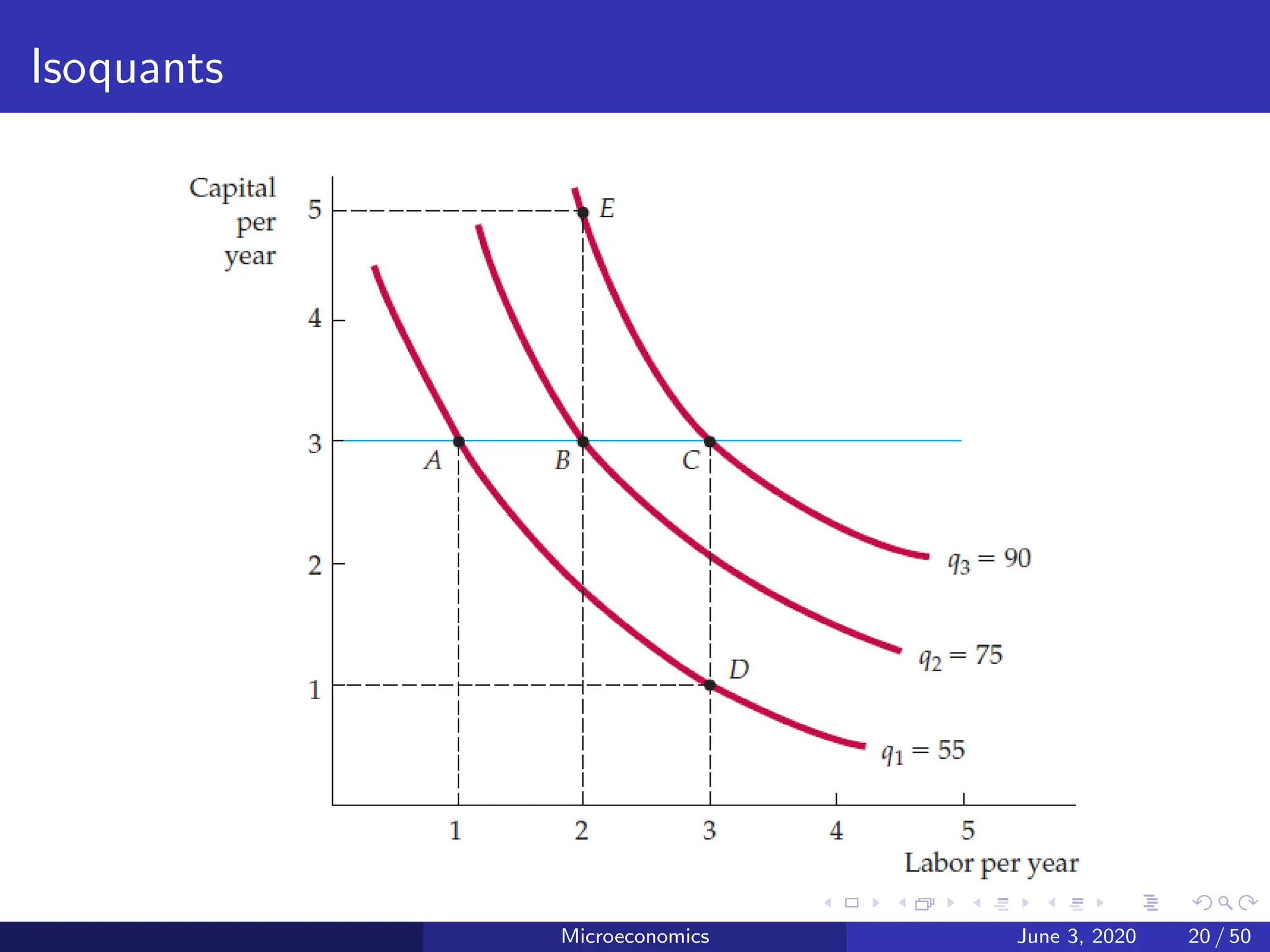
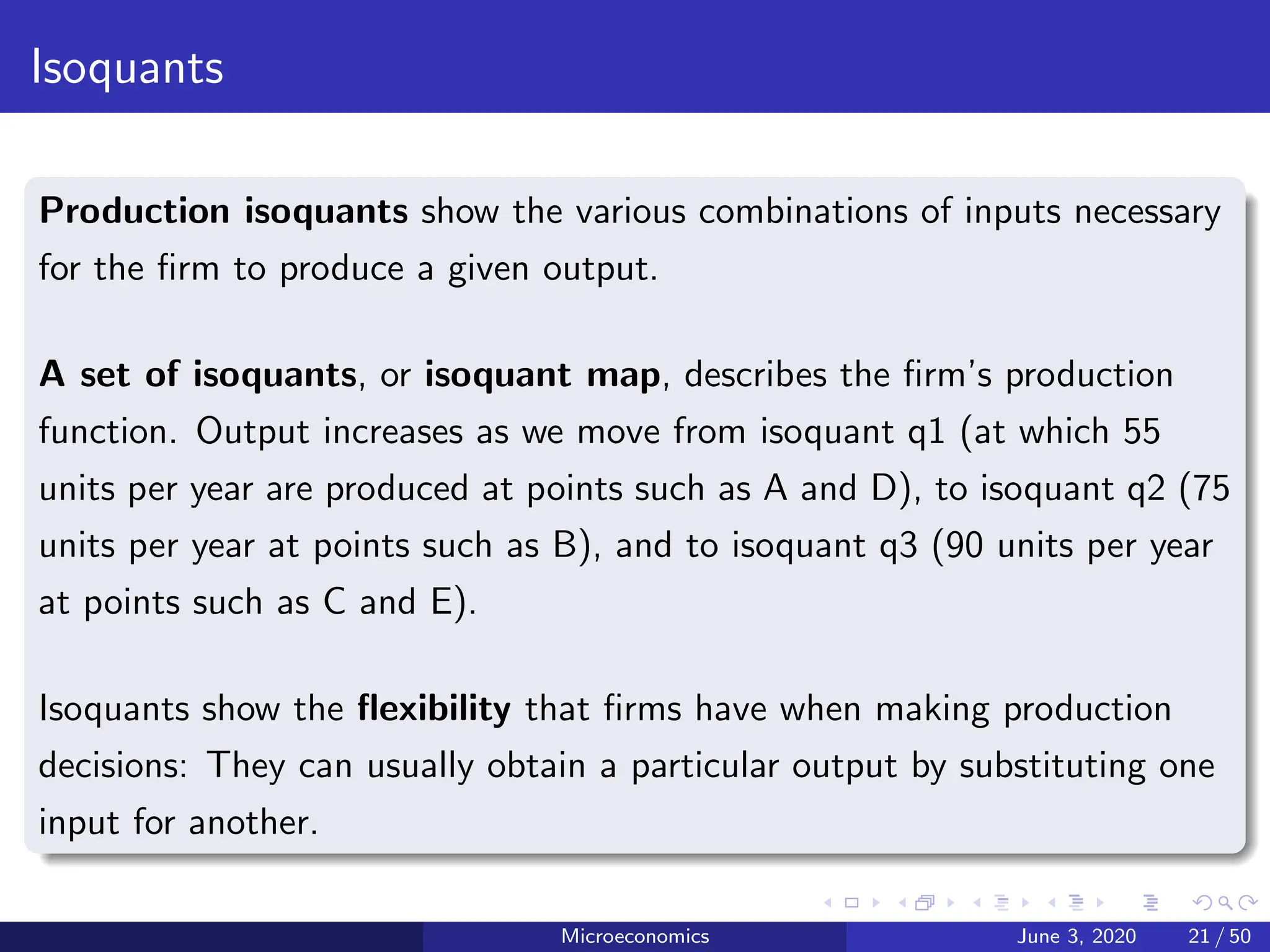
Production isoquants showthe various combinations of inputs necessary
for the firm to produce a given output.
A set of isoquants, or isoquant map, describes the firm’s production
function. Output increases as we move from isoquant q1 (at which 55
units per year are produced at points such as A and D), to isoquant q2 (75
units per year at points such as B), and to isoquant q3 (90 units per year
at points such as C and E).
Isoquants show the flexibility that firms have when making production
decisions: They can usually obtain a particular output by substituting one
input for another.
Microeconomics June 3, 2020 21 / 50
22.
Substitution Among Inputs
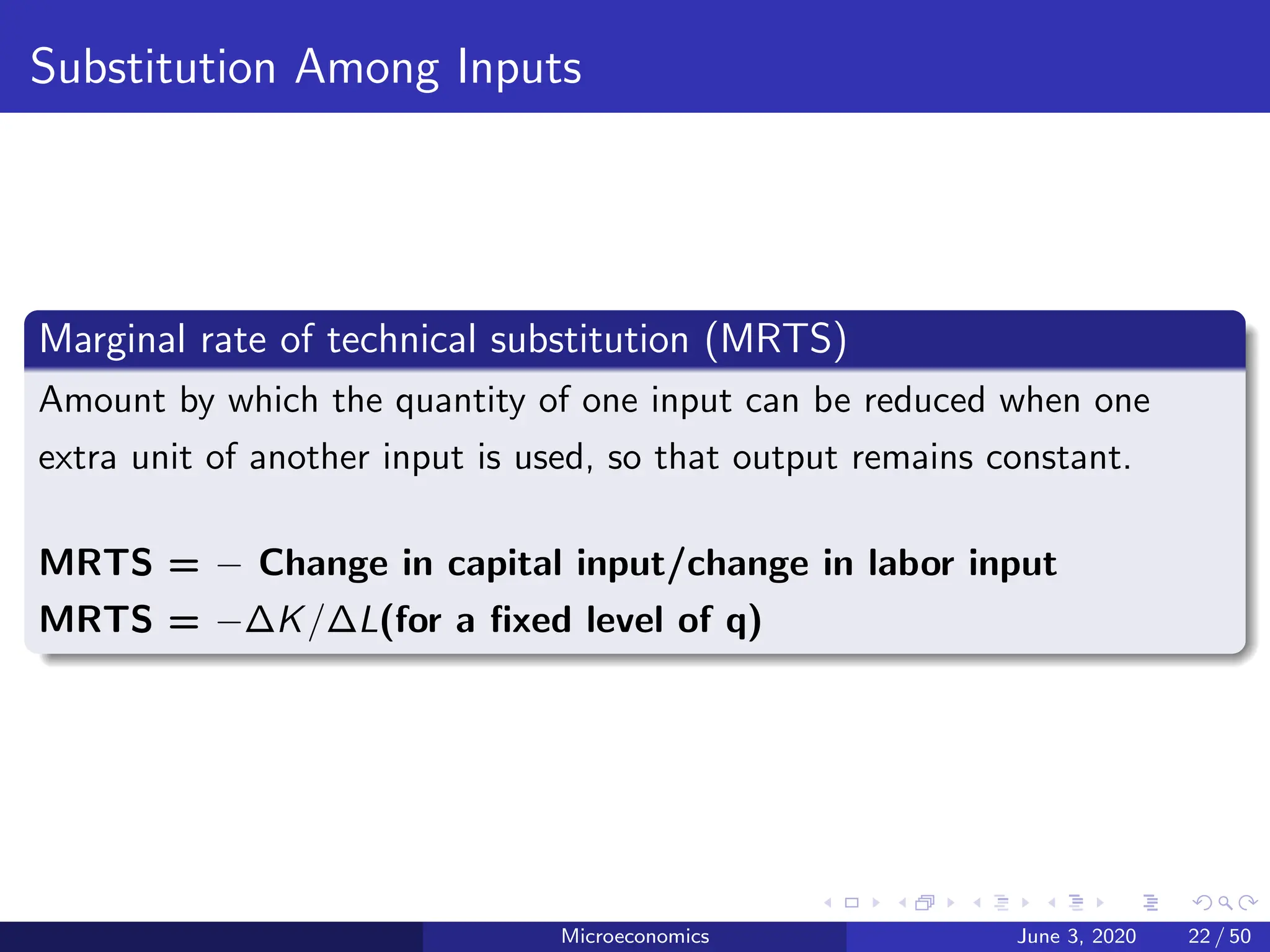
Marginalrate of technical substitution (MRTS)
Amount by which the quantity of one input can be reduced when one
extra unit of another input is used, so that output remains constant.
MRTS = − Change in capital input/change in labor input
MRTS = −∆K/∆L(for a fixed level of q)
Microeconomics June 3, 2020 22 / 50
Marginal rate oftechnical substitution (MRTS)
The slope of the isoquant at any point measures the marginal rate of
technical substitution—the ability of the firm to replace capital with labor
while maintaining the same level of output. On isoquant q2, the MRTS
falls from 2 to 1 to 2/3 to 1/3.
Microeconomics June 3, 2020 24 / 50
25.
Diminishing MRTS
The MRTSfalls as moving down along an isoquant. The mathematical
implication is that isoquants, like indifference curves, are convex, or bowed
inward. This is indeed the case for most production technologies.
The diminishing MRTS tells us that the productivity of any one input is
limited. As more and more labor is added to the production process in
place of capital, the productivity of labor falls. Similarly, when more
capital is added in place of labor, the productivity of capital falls.
Production needs a balanced mix of both inputs.
Microeconomics June 3, 2020 25 / 50
26.
Diminishing MRTS
Additional outputfrom increased use of labor = MPL∆L
Reduction in output from decreased use of capital = - MPK ∆K
Because we are keeping output constant by moving along an isoquant, the
total change in output must be zero. Thus,
(MPL∆L) + (MPK ∆K) = 0
The marginal rate of technical substitution between two inputs is equal to
the ratio of the marginal products of the inputs:
(MPL)/(MPK ) = −(∆K/∆L) = MRTS
Microeconomics June 3, 2020 26 / 50
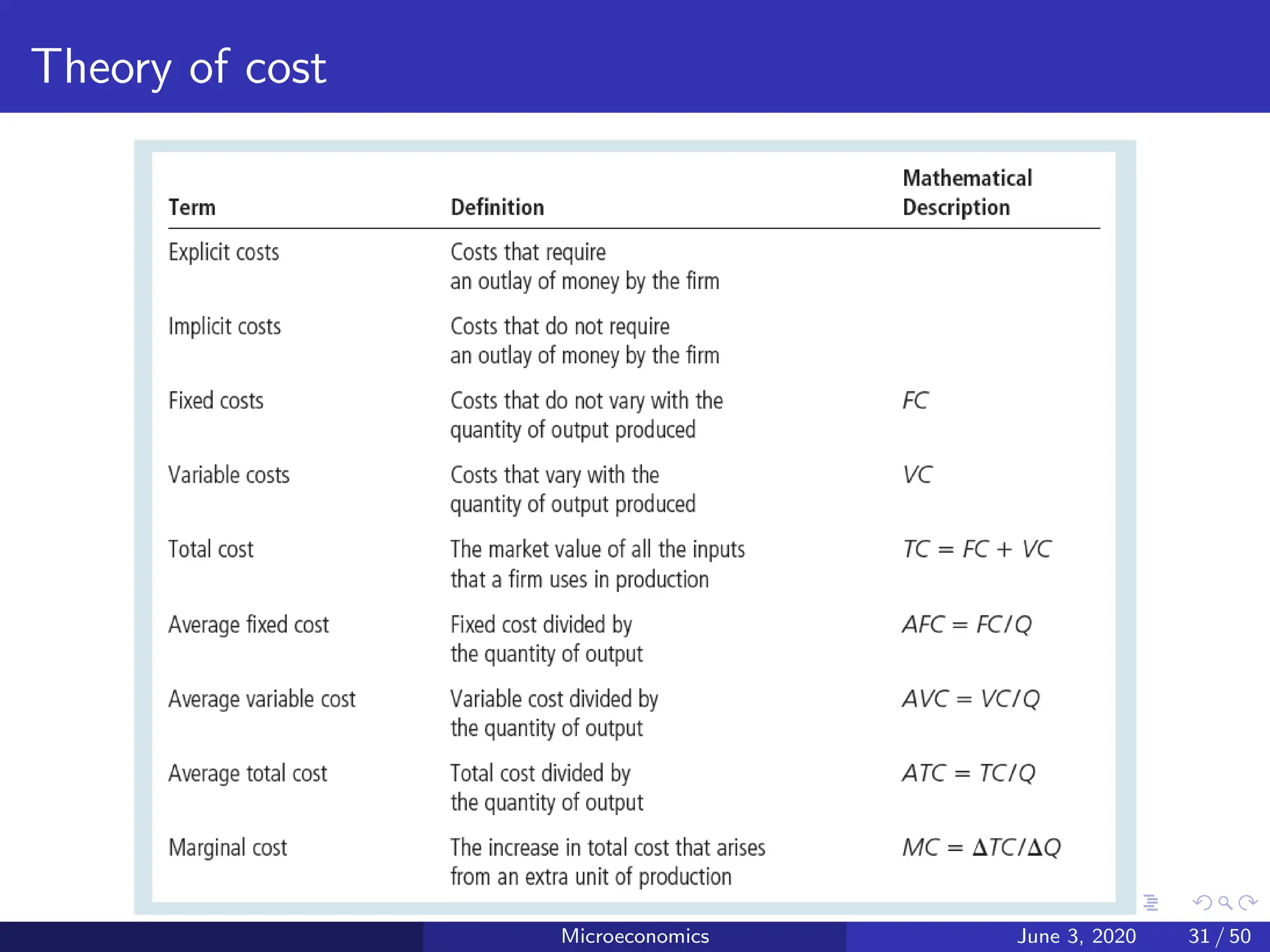
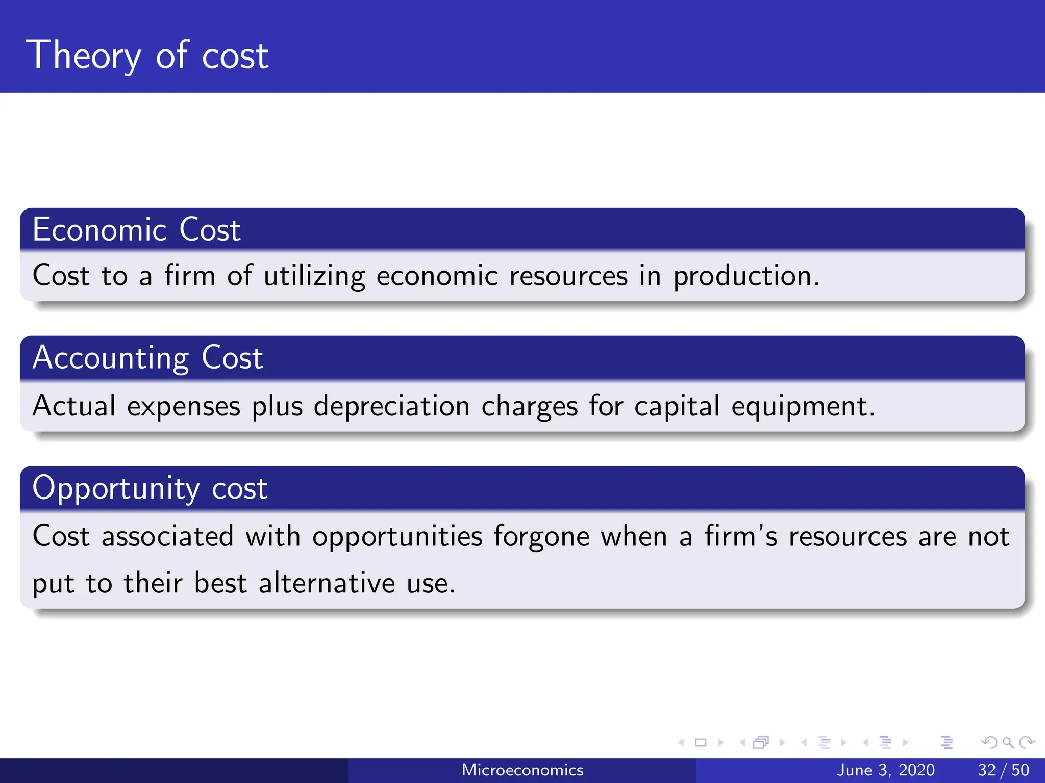
Theory of cost
EconomicCost
Cost to a firm of utilizing economic resources in production.
Accounting Cost
Actual expenses plus depreciation charges for capital equipment.
Opportunity cost
Cost associated with opportunities forgone when a firm’s resources are not
put to their best alternative use.
Microeconomics June 3, 2020 32 / 50
33.
Opportunity cost
Consider afirm that owns a building and therefore pays no rent for
office space. Does this mean the cost of office space is zero?
The firm’s managers and accountant might say yes, but an economist
would disagree. The economist would note that the firm could have
earned rent on the office space by leasing it to another company
Microeconomics June 3, 2020 33 / 50
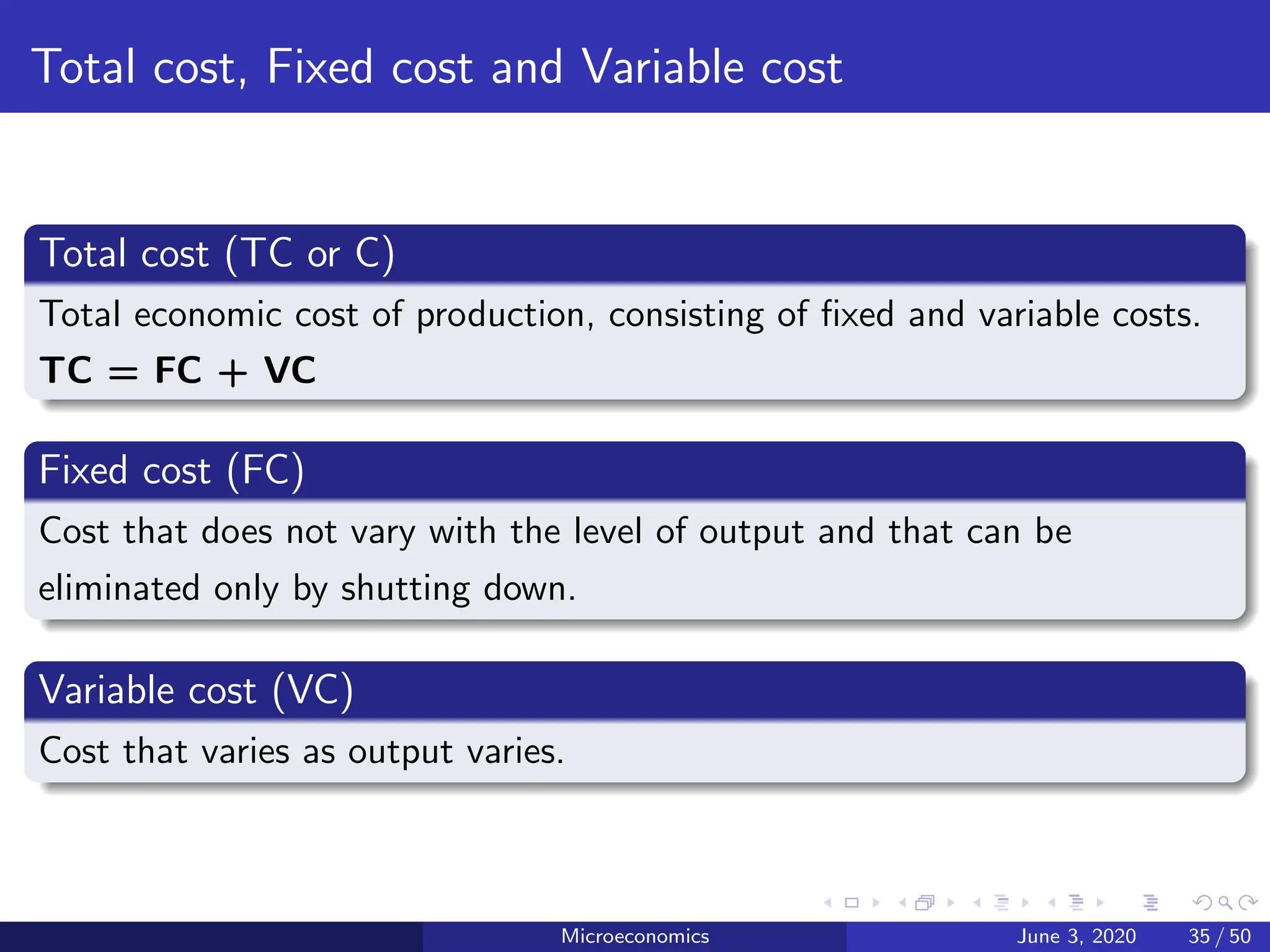
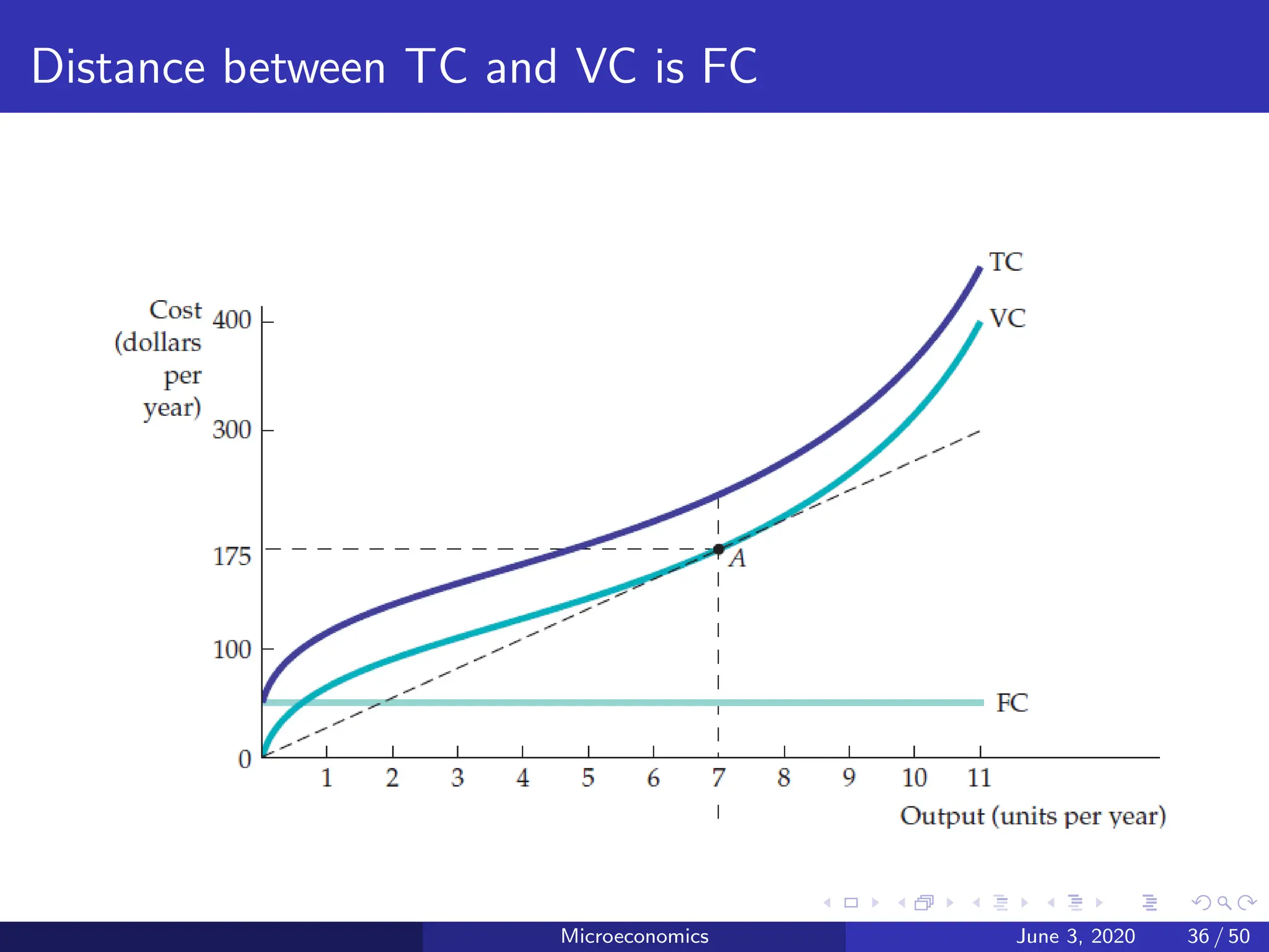
Total cost, Fixedcost and Variable cost
Total cost (TC or C)
Total economic cost of production, consisting of fixed and variable costs.
TC = FC + VC
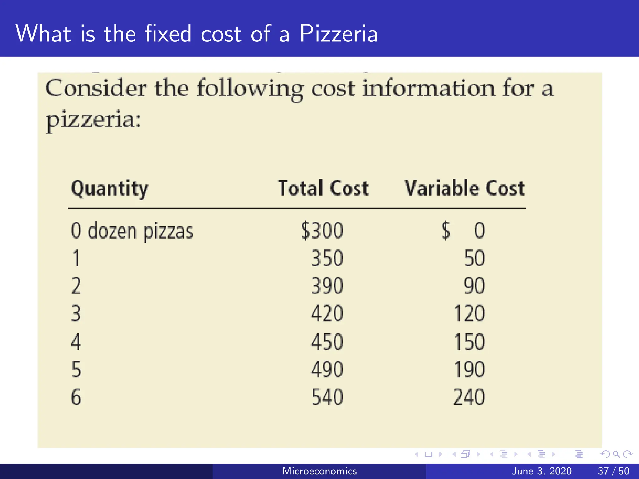
Fixed cost (FC)
Cost that does not vary with the level of output and that can be
eliminated only by shutting down.
Variable cost (VC)
Cost that varies as output varies.
Microeconomics June 3, 2020 35 / 50
What is thefixed cost of a Pizzeria
Microeconomics June 3, 2020 37 / 50
38.
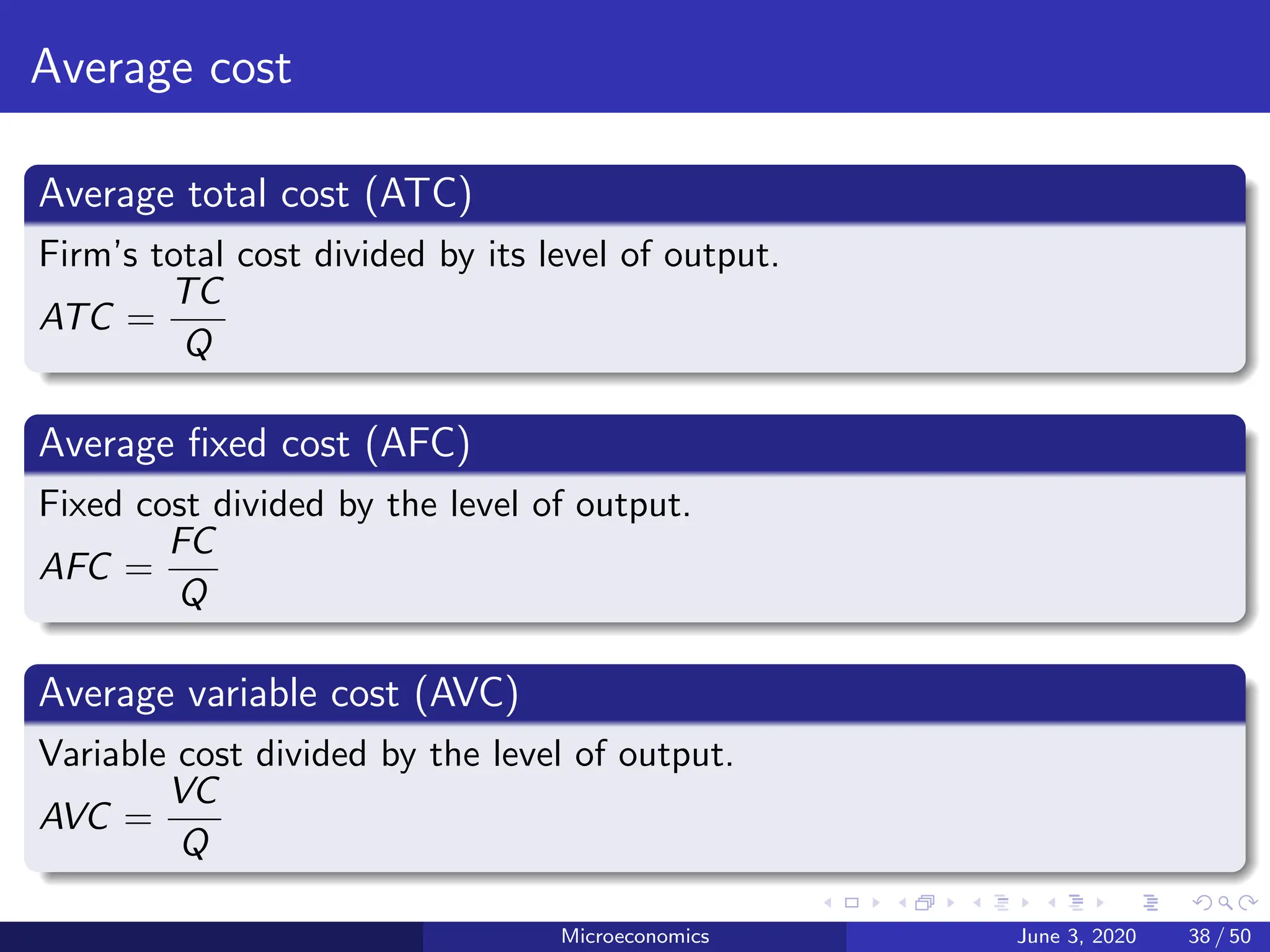
Average cost
Average totalcost (ATC)
Firm’s total cost divided by its level of output.
ATC =
TC
Q
Average fixed cost (AFC)
Fixed cost divided by the level of output.
AFC =
FC
Q
Average variable cost (AVC)
Variable cost divided by the level of output.
AVC =
VC
Q
Microeconomics June 3, 2020 38 / 50
39.
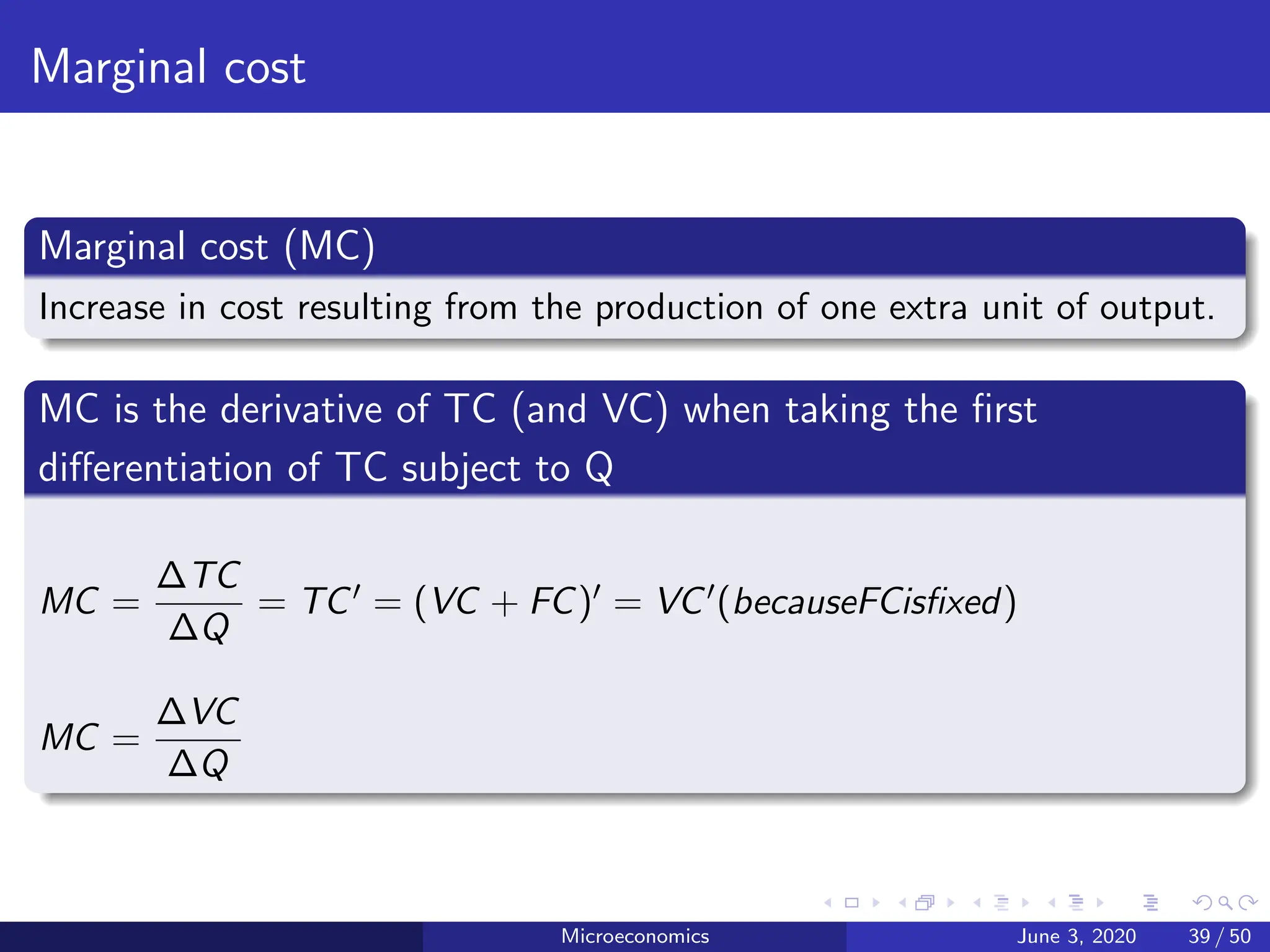
Marginal cost
Marginal cost(MC)
Increase in cost resulting from the production of one extra unit of output.
MC is the derivative of TC (and VC) when taking the first
differentiation of TC subject to Q
MC =
∆TC
∆Q
= TC0 = (VC + FC)0 = VC0(becauseFCisfixed)
MC =
∆VC
∆Q
Microeconomics June 3, 2020 39 / 50
40.
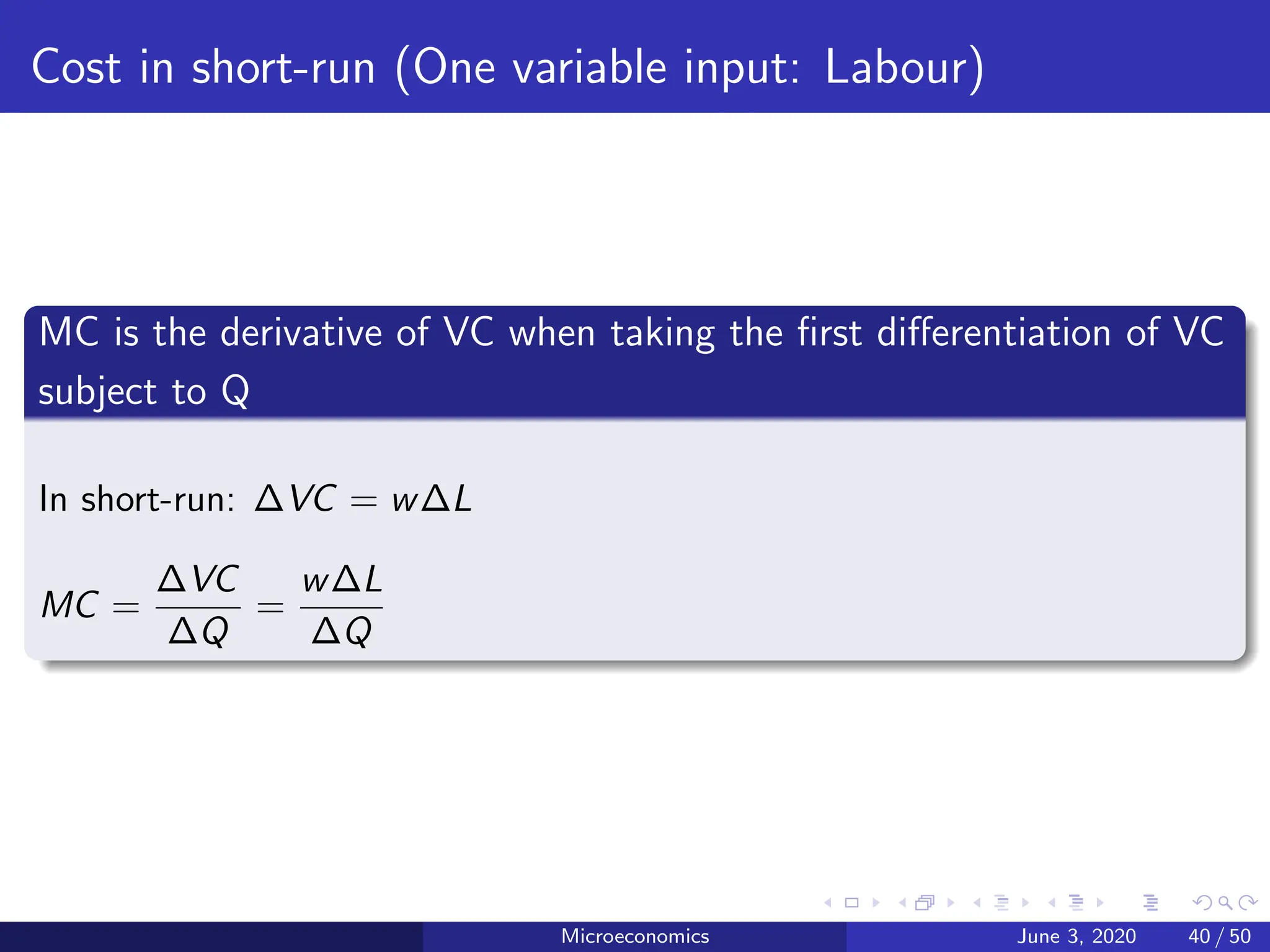
Cost in short-run(One variable input: Labour)
MC is the derivative of VC when taking the first differentiation of VC
subject to Q
In short-run: ∆VC = w∆L
MC =
∆VC
∆Q
=
w∆L
∆Q
Microeconomics June 3, 2020 40 / 50
41.
Diminishing marginal returnsand Marginal cost
Recall: Diminishing marginal returns means that the marginal product of
labor declines as the quantity of labor employed increases.
When there are diminishing marginal returns, marginal cost will
increase as output increases.
Microeconomics June 3, 2020 41 / 50
42.
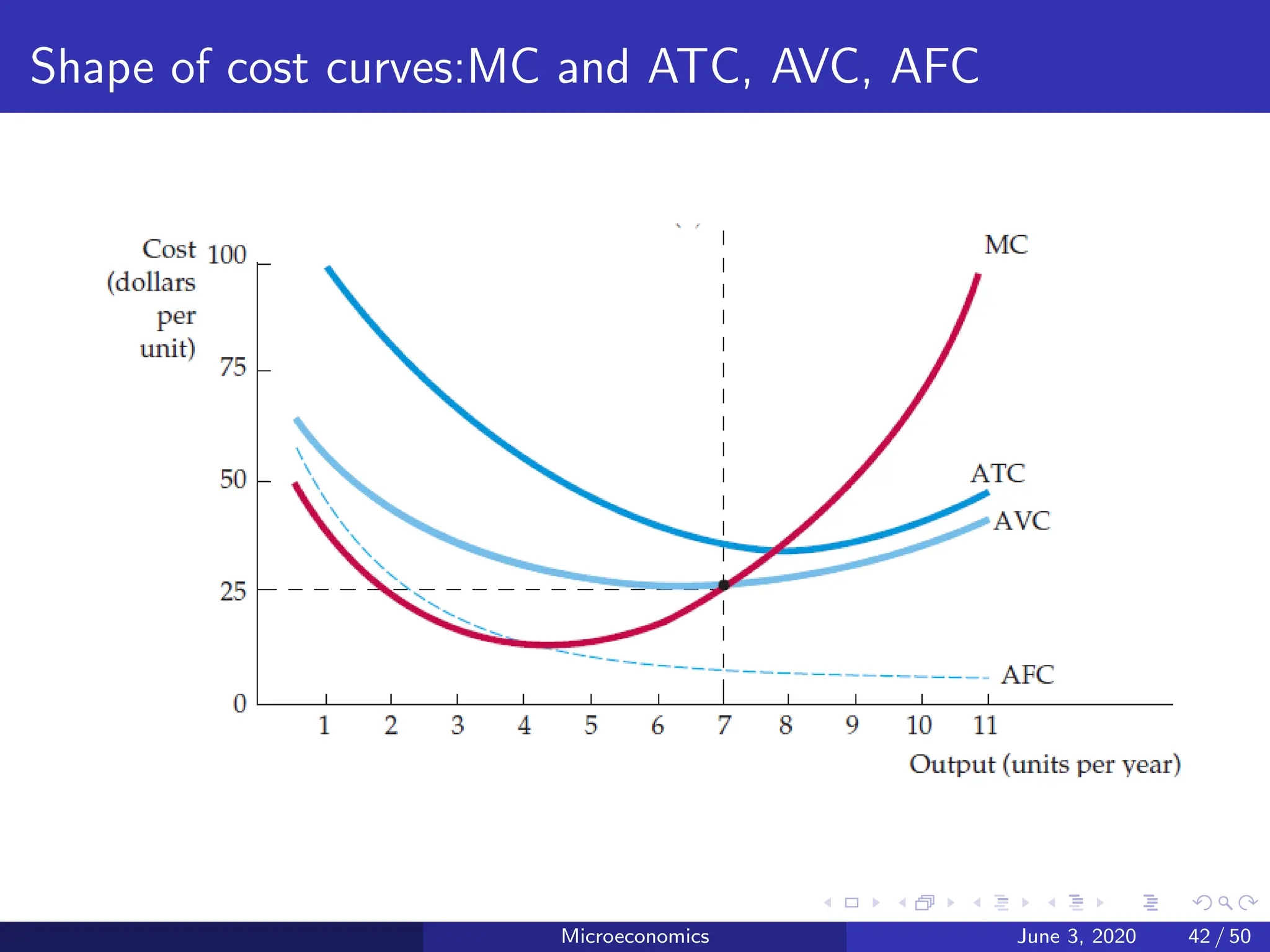
Shape of costcurves:MC and ATC, AVC, AFC
Microeconomics June 3, 2020 42 / 50
43.
MC crosses AVCand ATC at their minimum points
Average total cost ATC is the sum of average variable cost AVC and
average fixed cost AFC (vertically).
Marginal cost MC crosses the average variable cost and average total
cost curves at their minimum points.
Microeconomics June 3, 2020 43 / 50
44.
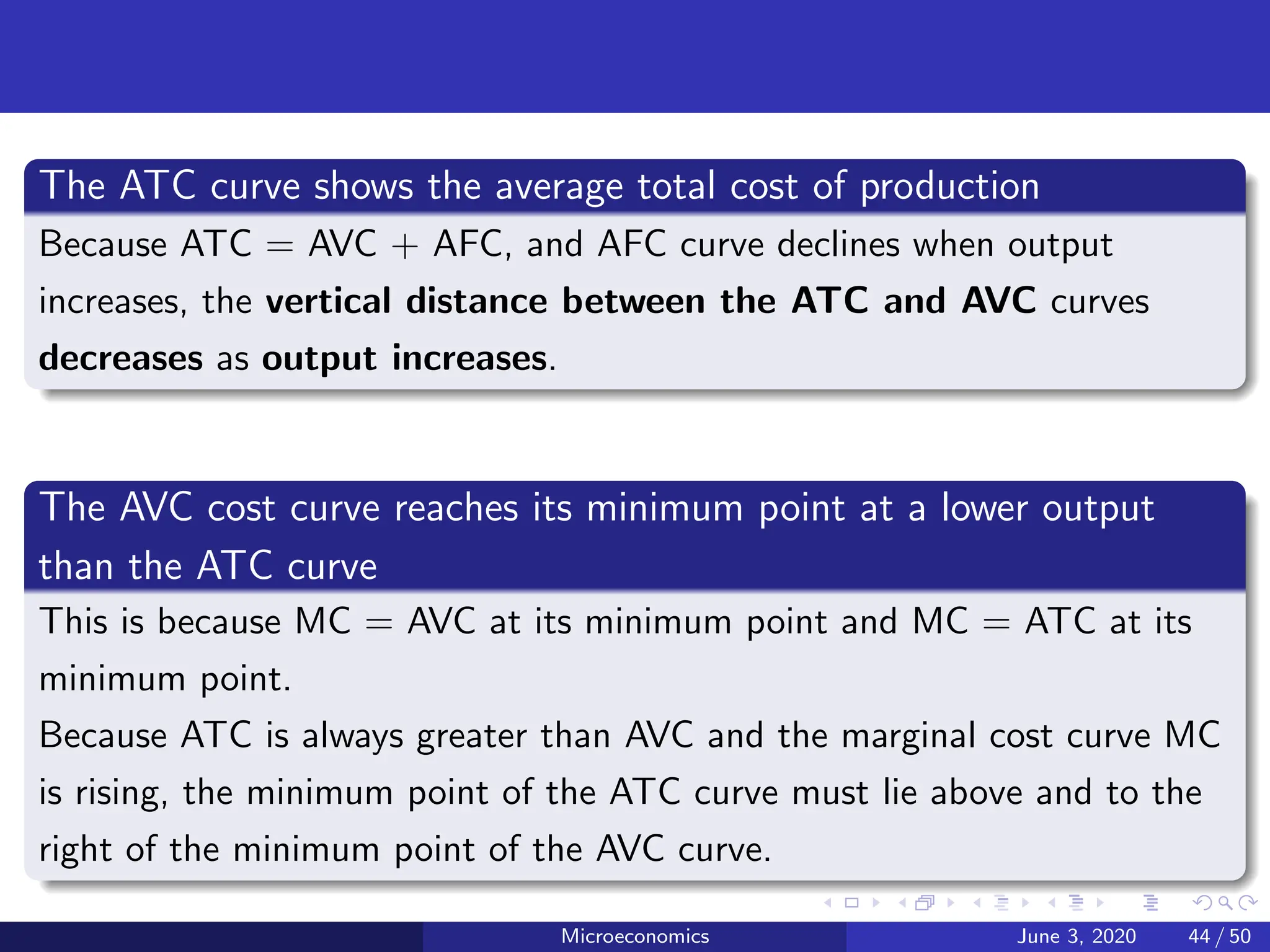
The ATC curveshows the average total cost of production
Because ATC = AVC + AFC, and AFC curve declines when output
increases, the vertical distance between the ATC and AVC curves
decreases as output increases.
The AVC cost curve reaches its minimum point at a lower output
than the ATC curve
This is because MC = AVC at its minimum point and MC = ATC at its
minimum point.
Because ATC is always greater than AVC and the marginal cost curve MC
is rising, the minimum point of the ATC curve must lie above and to the
right of the minimum point of the AVC curve.
Microeconomics June 3, 2020 44 / 50
45.
Cost in long-run
TheRelationship between Short-Run and Long-Run Average Total
Cost: Case study of car manufacturer Ford Motor Company
Over a period of only a few months, Ford cannot adjust the number or
size of its car factories. The only way it can produce additional cars is to
hire more workers at the factories it already has. The cost of these
factories is, therefore, a fixed cost in the short run. By contrast, over a
period of several years, Ford can expand the size of its factories, build new
factories, or close old ones. The cost of its factories is a variable cost in
the long run.
Microeconomics June 3, 2020 45 / 50
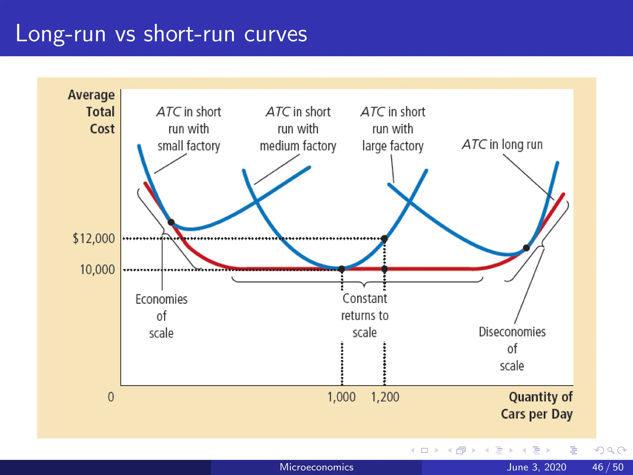
Long-run vs short-runcurves
The long-run average-total-cost curve is a much flatter U-shape than
the short-run average-total cost curve.
In addition, all the short-run curves lie on or above the long-run
curve. These properties arise because firms have greater flexibility in the
long run.
In essence, in the long run, the firm gets to choose which short-run curve
it wants to use. But in the short run, it has to use whatever short-run
curve it has chosen in the past.
Microeconomics June 3, 2020 47 / 50
48.
Economies and Diseconomiesof Scale
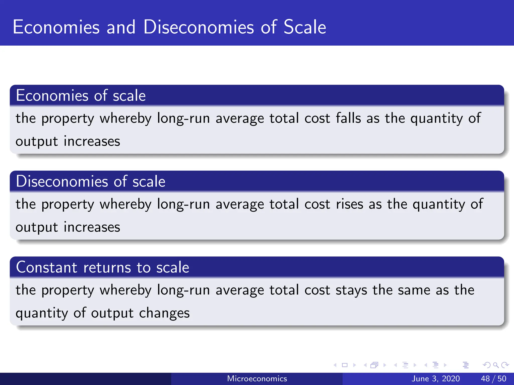
Economies of scale
the property whereby long-run average total cost falls as the quantity of
output increases
Diseconomies of scale
the property whereby long-run average total cost rises as the quantity of
output increases
Constant returns to scale
the property whereby long-run average total cost stays the same as the
quantity of output changes
Microeconomics June 3, 2020 48 / 50
49.
What might causeeconomies or diseconomies of scale?
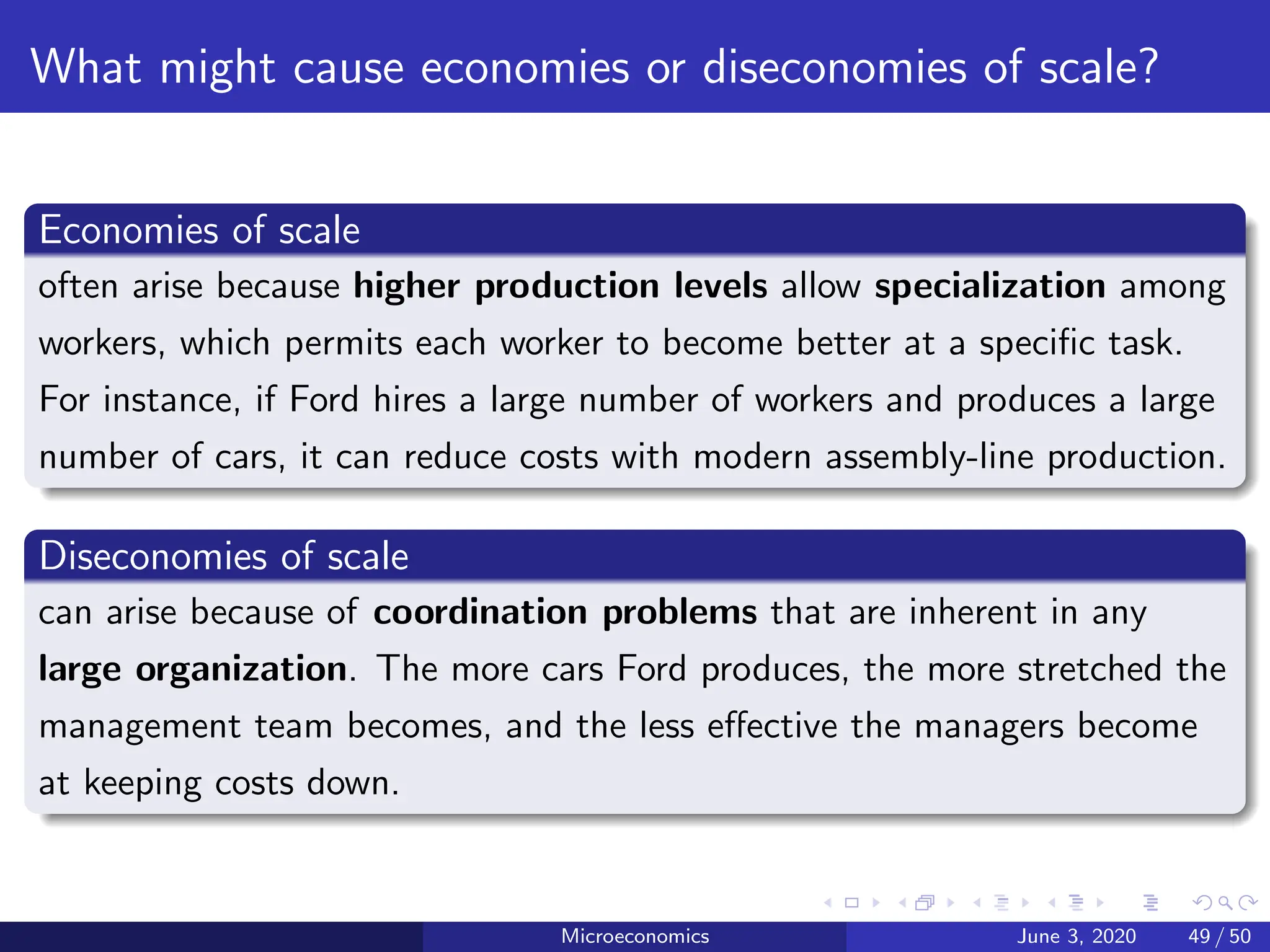
Economies of scale
often arise because higher production levels allow specialization among
workers, which permits each worker to become better at a specific task.
For instance, if Ford hires a large number of workers and produces a large
number of cars, it can reduce costs with modern assembly-line production.
Diseconomies of scale
can arise because of coordination problems that are inherent in any
large organization. The more cars Ford produces, the more stretched the
management team becomes, and the less effective the managers become
at keeping costs down.
Microeconomics June 3, 2020 49 / 50
50.
Does Boeing exhibiteconomies or diseconomies of scale?
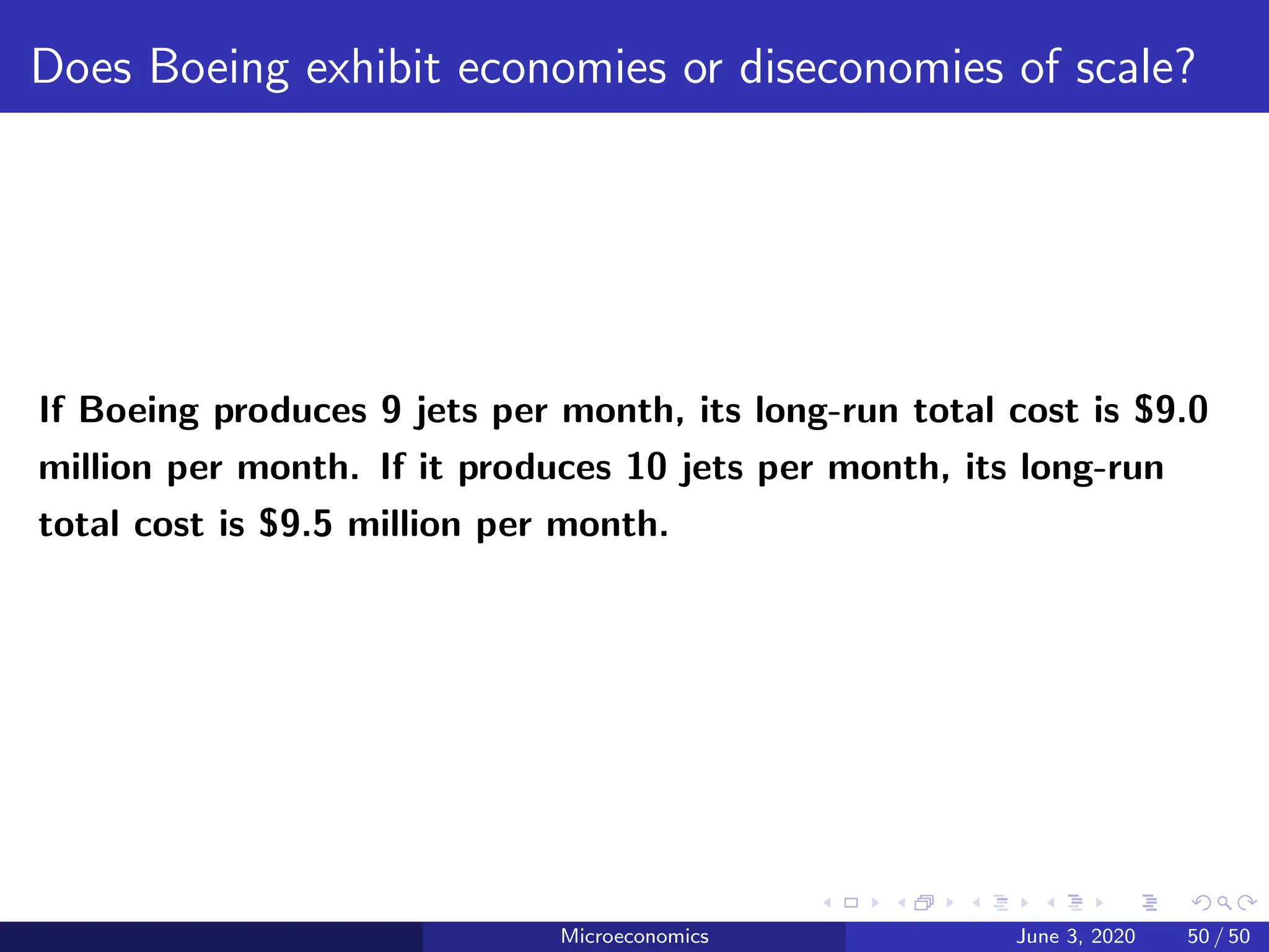
If Boeing produces 9 jets per month, its long-run total cost is $9.0
million per month. If it produces 10 jets per month, its long-run
total cost is $9.5 million per month.
Microeconomics June 3, 2020 50 / 50