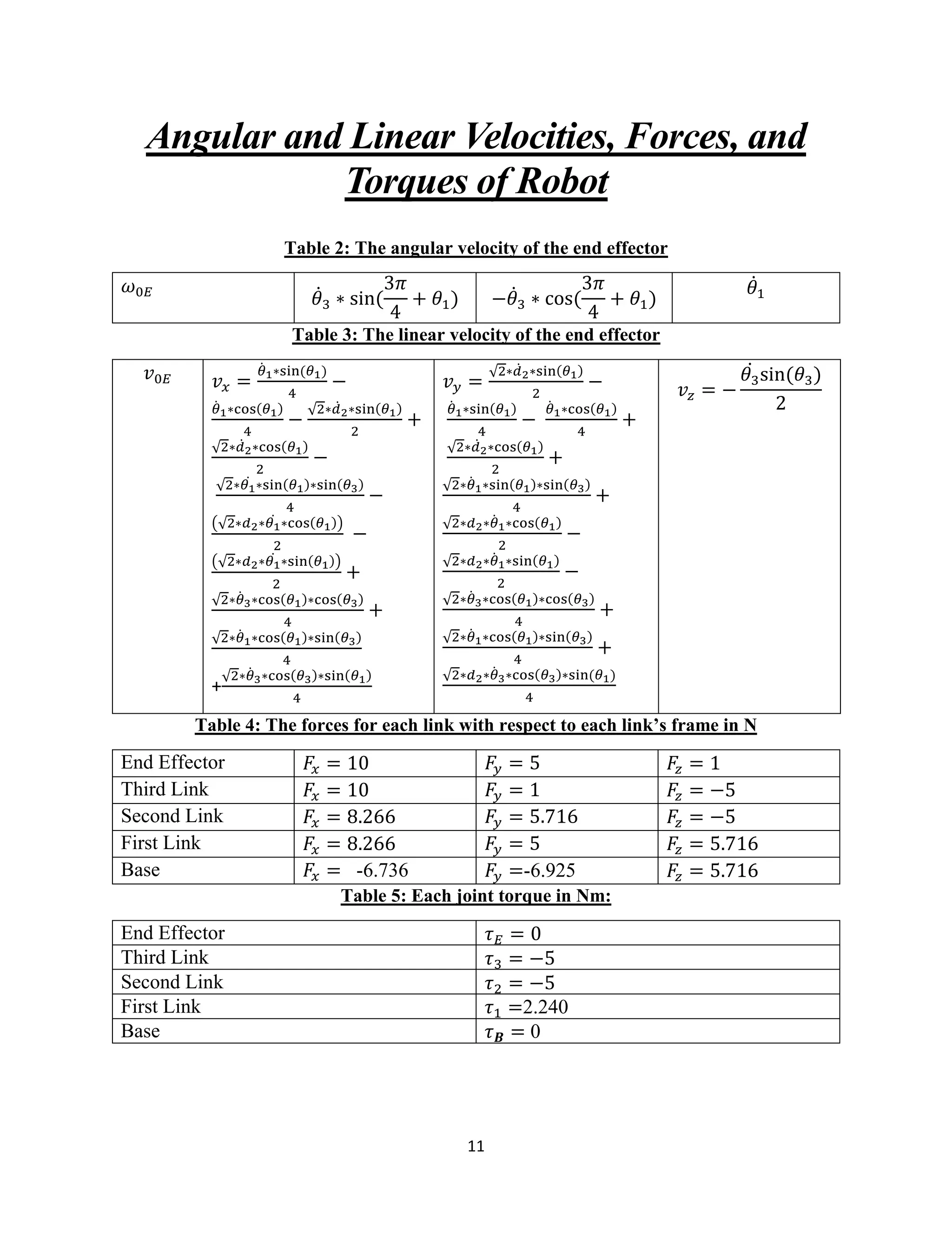
The document describes a 3 link robotic manipulator with revolute and prismatic joints. It provides the dimensions and D-H parameters of the robot, develops the forward kinematics equations relating the joint angles to the end effector pose, calculates the inverse kinematics, and determines the Jacobian and potential singularities. It also derives expressions for the angular and linear velocities of the end effector as well as the forces and torques throughout the robot.

1. 1
Model of Robotic Manipulator with Revolute and
Prismatic Joints
03/25/2016
Travis Heidrich
Report Contents:
Dimensions of the Robot 2
Denavit-Hartenberg Parameters 2-3
MATLAB Script 3-5
Frame Transformation Matrices 6
Reachable Workspace for Manipulator 7-8
Inverse Kinematics for Manipulator 8-9
Jacobian and Singularity 10
Angular and Linear Velocities, Forces, and Torques of Robot 11

2. 2
Dimensions of Robot
L1 = 1 m; L2 = 0.5 sin(45°) = 0.3536 m; LE = 0.5 m
D-H Parameters
Figure 1: Reference Frames and Dimensions of the three link robot

3. 3
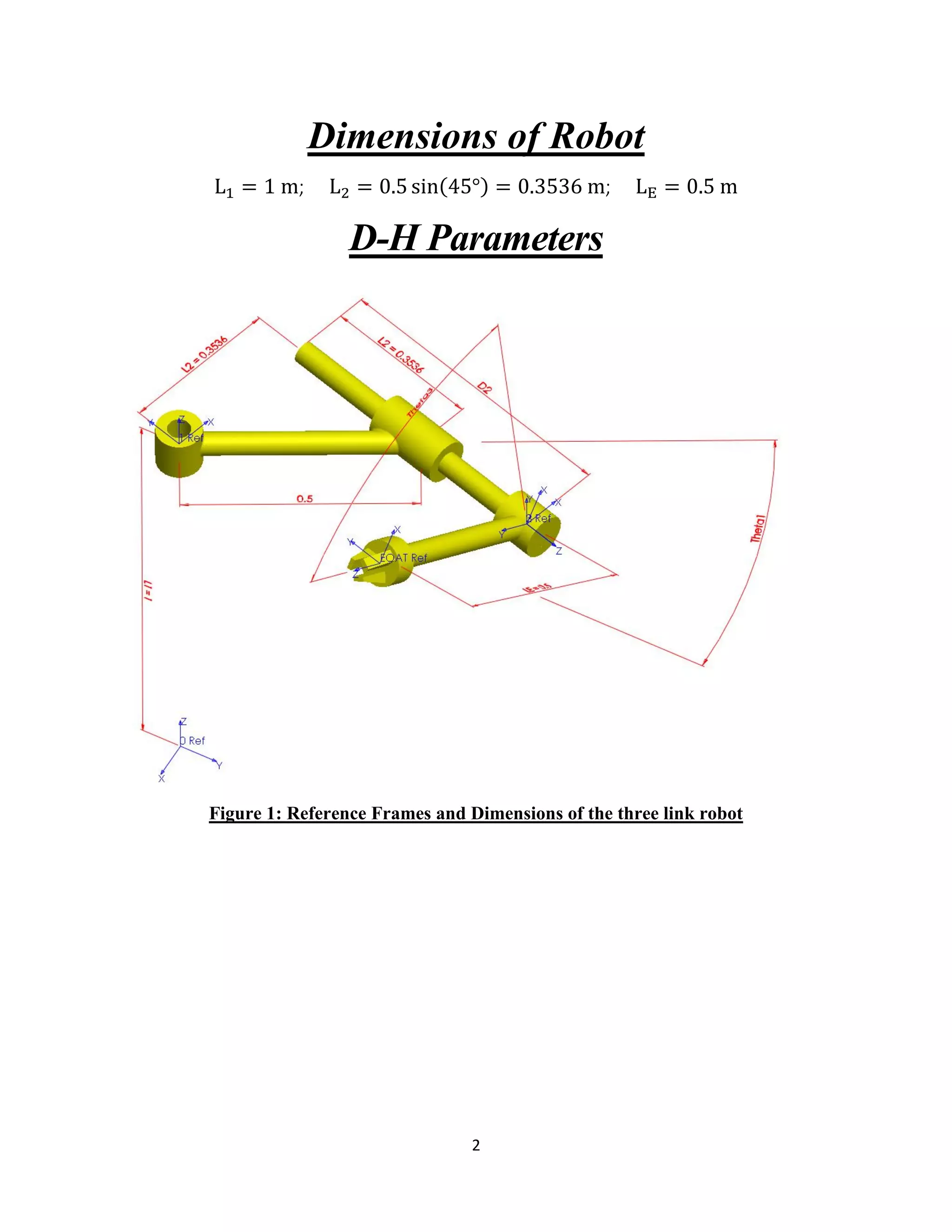
Table 1: D-H Parameter Table for all frames of the robot
i αi - 1 ai - 1 di - 1 θi
1 0 0 L1 θ1 + 135°
2 L2 90° d2 0
3 0 0 0 θ3
E 0 -90° LE 0
MatLab Script
%Solutions
clear all
close all
%Robot Dimensions
L_1 = 1; %meters
L_2 = 0.5*sind(45); %meters
L_E = 0.5; %meters
syms ai alphai di thetai theta1 d_2 theta3
T_x=[1 0 0 0;0 cos(alphai) -sin(alphai) 0;0 sin(alphai) cos(alphai) 0;0 0 0
1];
D_x=[1 0 0 ai;0 1 0 0;0 0 1 0;0 0 0 1];
T_z=[cos(thetai) -sin(thetai) 0 0;sin(thetai) cos(thetai) 0 0;0 0 1 0 ;0 0 0
1];
D_z=[1 0 0 0;0 1 0 0;0 0 1 di;0 0 0 1];
%Link the reference frames into one homogeneous transform matrix
AtB=T_x*D_x*T_z*D_z;
%Transformation from frame 0 to frame 1
ai = 0;
alphai = 0;
di = L1;
thetai = theta1 + 3*pi/4;
T_01 = subs(AtB);
iT_01 = inv(T_01);
%Transformation from frame 1 to frame 2
ai = L_2;
alphai = pi/2;
di = d_2;
thetai = 0;
T_12 = subs(AtB);
%iT_12 = inv(T_12);
%Transformation from frame 2 to frame 3
ai = 0;

4. 4
alphai = 0;
di = 0;
thetai = theta3;
T_23 = subs(AtB);
%Transformation from frame 3 to frame E
ai = 0;
alphai = -pi/2;
di = LE;
thetai = 0;
T3E = subs(AtB);
%iT3E = inv(T3E);
% Linking the Transformations
T_02 = T_01*T_12;
T_03 = T_01*T_12*T_23;
T_0E = T_01*T_12*T_23*T_3E;
T_1E = T_12*T_23*T_3E;
T_2E = T_23*T_3E;
x = T_0E(1,4);
y = T_0E(2,4);
z = T_0E(3,4);
%Inverse Kinematics for robot
syms px py pz
theta3 = solve( pz == z, theta3);
[d_2, theta1] = solve(px == x, py == y, d_2, theta1);
%Rotation Matrices frame to frame
R_01 = T_01(1:3,1:3);
R_12 = T_12(1:3,1:3);
R_23 = T_23(1:3,1:3);
R_3E = T_3E(1:3,1:3);
R_02 = R_01*R_12;
R_03 = R_01*R_12*R_23;
R_0E = R_01*R_12*R_23*R_3E;
%Forces 10,5,and 1
f_EE = [10;5;1];
f_33 = R_3E*f_EE;
f_22 = R_23*f_33;
f_11 = R_12*f_22;
f_00 = R_01*f_11;
%Vectors between D-H Origins
P_01 = T_01(1:3,4);
P_12 = T_12(1:3,4);
P_23 = T_23(1:3,4);
P_3E = T_3E(1:3,4);
P_00 = [0;0;0];
P_02 = T_02(1:3,4);
P_03 = T_03(1:3,4);
P_0E = T_0E(1:3,4);

5. 5
%Robot Torques
n_EE = zeros(3,1);
n_33 = R_01*n_EE + cross(P_3E,f_33);
n_22 = R_01*n_33 + cross(P_23,f_22);
n_11 = R_01*n_22 + cross(P_12,f_11);
n_00 = R_01*n_11 + cross(P_01,f_00);
t_0 = transpose(n_00)*[0;0;1];
t_1 = transpose(n_11)*[0;0;1];
t_2 = transpose(f_22)*[0;0;1];
t_3 = transpose(n_33)*[0;0;1];
t_E = zeros(3,1);
%Velocities
syms theta1Dot theta2Dot theta3Dot d_2Dot
%Unit Vectors
u_i = [1;0;0];
u_j = [0;1;0];
u_k = [0;0;1];
%Angular rotations
z_00 = u_k;
z_01 = R_01*u_k;
z_02 = R_02*u_k; %Prismatic
z_03 = R_03*u_k;
J_angular = [z00, 0*z01, z02];
Omega_0E = theta1Dot*u_k + 0 + theta3Dot*R_02*u_k + 0;
%Linear
J_linear = [cross(z_00,P_0E – P_00), z_02, cross(z_02,P_0E – P_02)];
%linear velocity equations
W_00 = zeros(3,1);
w_11 = inv(R_01)*w_00+[0;0;1]*theta1Dot;
w_22 = inv(R_12)*w_11+[0;0;0]*theta2Dot;
w_33 = inv(R_23)*w_22+[0;0;1]*theta3Dot;
w_EE = zeros(3,1);
v_00 = zeros(3,1);
v_11 = inv(R_01)*(v_00+cross(w_00,P_01));
v_22 = inv(R_12)*(v_11+cross(w_11,P_12))+d_2Dot*[0;0;1]; %Prismatic
v_33 = inv(R_23)*(v_22+cross(w_22,P_23));
v_EE = inv(R_3E)*(v_33+cross(w_33,P_3E));
v_0E = R_0E*v_EE;

6. 6
Frame Transformation Matrices
𝑇0
1
=
[
−sin (
𝜋
4
+ 𝜃1) −cos (
𝜋
4
+ 𝜃1) 0 0
cos (
𝜋
4
+ 𝜃1) − sin (
𝜋
4
+ 𝜃1) 0 0
0 0 1 1
0 0 0 1]
𝑇1
2
=
[
1 0 0
√2
4
0 0 −1 −𝑑2
0 1 0 0
0 0 0 1 ]
𝑇2
3
= [
cos(𝜃3) −sin(𝜃3) 0 0
sin(𝜃3) cos(𝜃3) 0 0
0 0 1 0
0 0 0 1
]
𝑇3
𝐸
=
[
1 0 0 0
0 0 1
1
2
0 0 1 0
0 0 0 1]
𝑇0
𝐸
=
[
− cos(𝜃3) ∗ sin(
𝜋
4
+ 𝜃1) −cos(
𝜋
4
+ 𝜃1) sin(𝜃3) ∗ sin (
𝜋
4
+ 𝜃1)
(sin(𝜃3) ∗ sin(
𝜋
4
+ 𝜃1))
2
+ 𝑑2 ∗ cos (
𝜋
4
+ 𝜃1) −
(√2 ∗ sin(
𝜋
4
+ 𝜃1))
4
cos(𝜃3) ∗ sin(
𝜋
4
+ 𝜃1) −𝑠𝑖𝑛(
𝜋
4
+ 𝜃1) − cos (
𝜋
4
+ 𝜃1) ∗ sin(𝜃3)
(√2 ∗ cos (
𝜋
4
+ 𝜃1))
4
−
(cos (
𝜋
4
+ 𝜃1) ∗ sin(𝜃3))
2
+ 𝑑2 ∗ sin(
𝜋
4
+ 𝜃1)
sin(𝜃3) 0 cos(𝜃3)
cos(𝜃3)
2
+ 1
0 0 0 1 ]

7. 7
Reachable Workspace for Manipulator
Figure 2: X-Z Plane View of reachable workspace
Figure 3: X-Y Plane View of reachable workspace

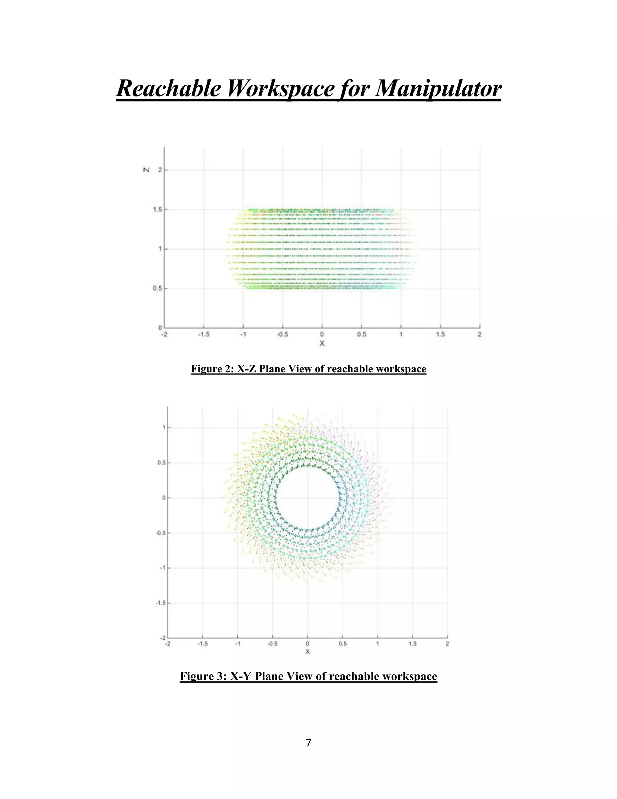
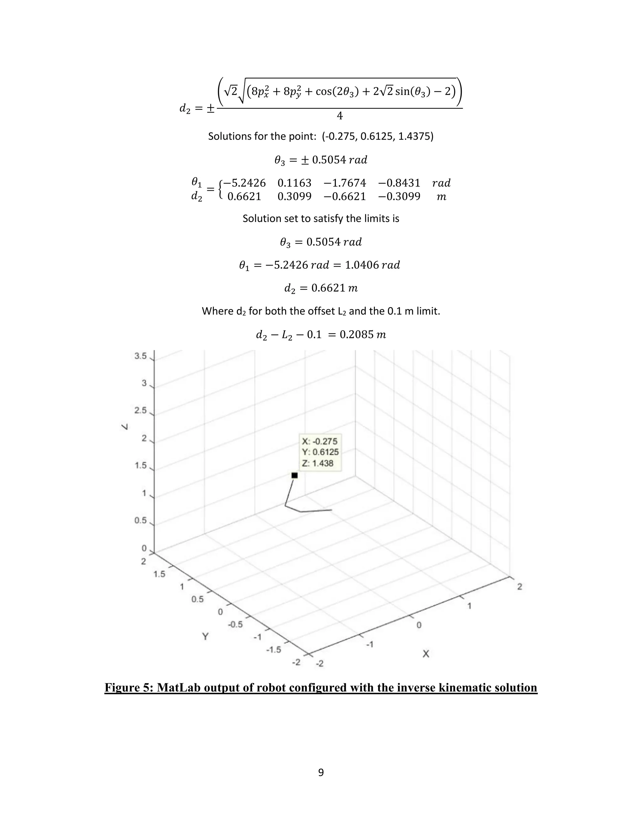
8. 8
Figure 4: Trimetric view of reachable workspace
Inverse Kinematics for Manipulator
𝑇0
𝐸
= [
𝑟11 𝑟12 𝑟13 𝑝 𝑥
𝑟21 𝑟22 𝑟23 𝑝 𝑦
𝑟31 𝑟32 𝑟33 𝑝𝑧
0 0 0 1
]
𝑝𝑧 =
cos(𝜃3)
2
+1
𝑝 𝑦 =
(√2 𝑐𝑜𝑠 (
𝜋
4 + 𝜃1))
4
−
( 𝑐𝑜𝑠 (
𝜋
4 + 𝜃1) 𝑠𝑖𝑛(𝜃3))
2
+ 𝑑2 𝑠𝑖𝑛 (
𝜋
4
+ 𝜃1)
𝑝 𝑥 =
( 𝑠𝑖𝑛(𝜃3) 𝑠𝑖𝑛 (
𝜋
4 + 𝜃1))
2
−
(√2 𝑠𝑖𝑛 (
𝜋
4 + 𝜃1))
4
+ 𝑑2 𝑐𝑜𝑠 (
𝜋
4
+ 𝜃1)
Solving for θ3
𝜃3 = ± cos−1(2𝑝𝑧 − 2)
Substituting θ3 and solving for θ1 and d2
𝜃1 = 2 tan−1
(4𝑝 𝑦 ± √2√(8𝑝 𝑥
2 − 2√2 sin(𝜃3) + cos(2𝜃3) + 8𝑝 𝑦
2 − 2)) −
3𝜋
4

9. 9
𝑑2 = ±
(√2√(8𝑝 𝑥
2 + 8𝑝 𝑦
2 + cos(2𝜃3) + 2√2 sin(𝜃3) − 2))
4
Solutions for the point: (-0.275, 0.6125, 1.4375)
𝜃3 = ± 0.5054 𝑟𝑎𝑑
𝜃1
𝑑2
= {
−5.2426 0.1163 −1.7674 −0.8431 𝑟𝑎𝑑
0.6621 0.3099 −0.6621 −0.3099 𝑚
Solution set to satisfy the limits is
𝜃3 = 0.5054 𝑟𝑎𝑑
𝜃1 = −5.2426 𝑟𝑎𝑑 = 1.0406 𝑟𝑎𝑑
𝑑2 = 0.6621 𝑚
Where d2 for both the offset L2 and the 0.1 m limit.
𝑑2 − 𝐿2 − 0.1 = 0.2085 𝑚
Figure 5: MatLab output of robot configured with the inverse kinematic solution

10. 10
Jacobian
[
cos (
𝜋
4
+ 𝜃1) ∗ sin(𝜃3)
2
−
√2 ∗ cos (
𝜋
4
+ 𝜃1)
4
− 𝑑2 ∗ sin (
𝜋
4
+ 𝜃1) cos (
𝜋
4
+ 𝜃1)
cos(𝜃3) ∗ sin (
𝜋
4
+ 𝜃1)
2
sin(𝜃3) ∗ sin (
𝜋
4 + 𝜃1)
2
−
√2 ∗ sin (
𝜋
4 + 𝜃1)
4
+ 𝑑2 ∗ cos (
𝜋
4
+ 𝜃1) sin(
𝜋
4
+ 𝜃1) −
cos(𝜃3) ∗ cos (
𝜋
4 + 𝜃1)
2
0 0
− sin(𝜃3)
2
0 0 − cos (
𝜃
4
+ 𝜃1)
0 0 sin (
𝜃
4
+ 𝜃1)
1 0 0 ]
𝐷𝑒𝑡(𝐽𝑙𝑖𝑛𝑒𝑎𝑟) =
𝑑2 ∗ sin(𝜃3)
2
𝐷𝑒𝑡(𝐽 𝑎𝑛𝑔𝑢𝑙𝑎𝑟) = 0
Singularities
When determinate of Jacobian = 0
The was no determinate for the angular Jacobian
There was no theta 1 that resulted in singularities
Given theta3 = 0 and pi
For d_2 < = 0.5(sin(45)) + 0.1
OR
d_2 > 0.5(sin(45)) + 0.5

11. 11
Angular and Linear Velocities, Forces, and
Torques of Robot
Table 2: The angular velocity of the end effector
𝜔0𝐸
𝜃̇3 ∗ sin(
3𝜋
4
+ 𝜃1) −𝜃̇3 ∗ cos(
3𝜋
4
+ 𝜃1)
𝜃̇1
Table 3: The linear velocity of the end effector
𝑣0𝐸 𝑣 𝑥 =
𝜃̇1∗sin(𝜃1)
4
−
𝜃̇1∗cos(𝜃1)
4
−
√2∗𝑑̇2∗sin(𝜃1)
2
+
√2∗𝑑̇2∗cos(𝜃1)
2
−
√2∗𝜃1
̇ ∗sin(𝜃1)∗sin(𝜃3)
4
−
(√2∗𝑑2∗𝜃1
̇ ∗cos(𝜃1))
2
−
(√2∗𝑑2∗𝜃1
̇ ∗sin(𝜃1))
2
+
√2∗𝜃̇3∗cos(𝜃1)∗cos(𝜃3)
4
+
√2∗𝜃̇1∗cos(𝜃1)∗sin(𝜃3)
4
+
√2∗𝜃̇3∗cos(𝜃3)∗sin(𝜃1)
4
𝑣 𝑦 =
√2∗𝑑̇2∗sin(𝜃1)
2
−
𝜃̇1∗sin(𝜃1)
4
−
𝜃̇1∗cos(𝜃1)
4
+
√2∗𝑑̇2∗cos(𝜃1)
2
+
√2∗𝜃̇1∗sin(𝜃1)∗sin(𝜃3)
4
+
√2∗𝑑2∗𝜃̇1∗cos(𝜃1)
2
−
√2∗𝑑2∗𝜃̇1∗sin(𝜃1)
2
−
√2∗𝜃̇3∗cos(𝜃1)∗cos(𝜃3)
4
+
√2∗𝜃̇1∗cos(𝜃1)∗sin(𝜃3)
4
+
√2∗𝑑2∗𝜃̇3∗cos(𝜃3)∗sin(𝜃1)
4
𝑣𝑧 = −
𝜃3
̇ sin(𝜃3)
2
Table 4: The forces for each link with respect to each link’s frame in N
End Effector 𝐹𝑥 = 10 𝐹𝑦 = 5 𝐹𝑧 = 1
Third Link 𝐹𝑥 = 10 𝐹𝑦 = 1 𝐹𝑧 = −5
Second Link 𝐹𝑥 = 8.266 𝐹𝑦 = 5.716 𝐹𝑧 = −5
First Link 𝐹𝑥 = 8.266 𝐹𝑦 = 5 𝐹𝑧 = 5.716
Base 𝐹𝑥 = -6.736 𝐹𝑦 =-6.925 𝐹𝑧 = 5.716
Table 5: Each joint torque in Nm:
End Effector 𝜏 𝐸 = 0
Third Link 𝜏3 = −5
Second Link 𝜏2 = −5
First Link 𝜏1 =2.240
Base 𝜏 𝑩 = 0